Production Scheduling Nahmias, Chapter 8 ( D t lj l i ) (sv ...
Production Scheduling Nahmias, Chapter 8 ( D t lj l i ) (sv ...
Production Scheduling Nahmias, Chapter 8 ( D t lj l i ) (sv ...

Create successful ePaper yourself
Turn your PDF publications into a flip-book with our unique Google optimized e-Paper software.
.<br />
<strong>Production</strong> <strong>Scheduling</strong><br />
<strong>Nahmias</strong>, <strong>Chapter</strong> 8<br />
( (<strong>sv</strong>. Deta<strong>lj</strong>planering)<br />
D t <strong>lj</strong> l i )<br />
<strong>Production</strong> and Inventory Control (MPS)<br />
MIOF10<br />
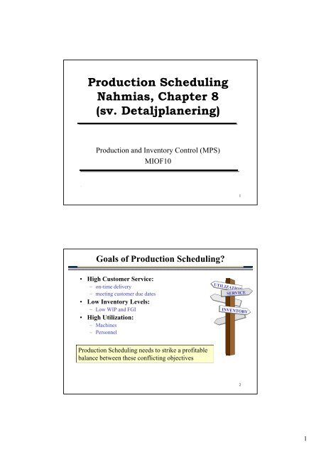
Goals of <strong>Production</strong> <strong>Scheduling</strong>?<br />
• High Customer Service:<br />
– on-time delivery<br />
– meeting customer due dates<br />
• Low Inventory Levels:<br />
– Low WIP and FGI<br />
• High Utilization:<br />
– Machines<br />
– Personnel<br />
<strong>Production</strong> <strong>Scheduling</strong> needs to strike a profitable<br />
balance between these conflicting objectives<br />
1<br />
2<br />
1
High Customer Service - Meeting Due dates<br />
• Service Level 1: • Lateness:<br />
– Particularly common in – Difference between order due date<br />
make to order systems. y<br />
and completion p date ( (can be<br />
– Fraction of orders which are positive).<br />
filled on or before their due – Average lateness has little meaning<br />
dates .<br />
by itself. Need also to consider the<br />
lateness variance.<br />
• Tardiness:<br />
• Service level 2:<br />
– Is equal to the lateness of a job if it is<br />
– Common in make to stock late and zero, otherwise.<br />
systems.<br />
– Average tardiness is meaningful but<br />
– Fraction of demands met<br />
from stock.<br />
unintuitive.<br />
<strong>Scheduling</strong> Approaches & Assumptions<br />
• <strong>Scheduling</strong> as practice dates back to Scientiffic Management<br />
– Serious analysis contingent on computer power - started in 1950’s<br />
• MRP/ERP:<br />
– Benefits: Simple paradigm, paradigm hierarchical approach. approach<br />
– Problems<br />
• MRP assumes that lead times are a constant attribute of the part,<br />
independent of the status of the shop (assumes infinite capacity).<br />
• Strong incentive to use pessimistic lead time estimates to hedge<br />
• Classic <strong>Scheduling</strong>: (only classic in academia)<br />
– Benefits: “Optimal” schedules (large integer programming problems)<br />
– Problems: Bad assumptions.<br />
• All jobs available at the start of the problem.<br />
• Deterministic processing times.<br />
• No setups.<br />
• No machine breakdowns.<br />
• No cancellation.<br />
3<br />
4<br />
2
Results for a Single Machine…<br />
• Minimizing Average Cycle Time per job:<br />
– Sequence the jobs in “shortest process time first” (SPT) order.<br />
– The makespan of the considered batch of jobs is not affected<br />
�� Th The makespan= k th the time ti to t process a defined d fi d set t of f jobs j b from f<br />
start to finish<br />
• Minimizing Maximum Lateness (or Tardiness):<br />
– Minimize by performing in “earliest due date” (EDD) order.<br />
– If there exists a sequence with no tardy jobs, EDD will do it.<br />
• Minimize the number of tardy jobs<br />
– Optimal schedule can easily be obtained using Moore’s algorithm<br />
• Mi Minimizing i i i Average A Tardiness: T di<br />
– No simple sequencing rule will work. Problem is NP Hard.<br />
Moore’s Algorithm<br />
• A method for minimizing the number of tardy jobs, when all<br />
jobs are considered equally important<br />
11. Od Order the h jjobs b according di to the h EDD rule. l<br />
2. Stop if no jobs are tardy – the optimal solution is found!<br />
Go to step 6.<br />
3. Find the first tardy job in the sequence.<br />
4. Assuming that this tardy job is the kth in the sequence. Find and<br />
remove job j (j=1, 2, 3, …, k) with the longest processing time.<br />
5. Revise the completion times and return to step 2<br />
6. Insert the removed jobs at the end of the sequence in the order they<br />
were removed<br />
5<br />
6<br />
3
Moore’s Example<br />
Start with EDD schedule<br />
Job Time Done Due Tardy<br />
2 2 2 6 0<br />
5 5 7 8 0<br />
3 3 10 9 1<br />
4 4 14 11 3<br />
1 6 20 18 2<br />
Job 3 is first late job.<br />
Job 5 is longest of jobs 2,5,3.<br />
Moore’s Example<br />
Job Time Done Due Tardy<br />
2 2 2 6 0<br />
3 3 5 9 0<br />
4 4 9 11 0<br />
1 6 15 18 0<br />
5 5 20 8 12<br />
Average Flow = 51 / 5 = 10.2<br />
Average tardiness = 12 / 5 = 2.4<br />
Number tardy = 1<br />
Max. Tardy =12<br />
4
Results for Two Machines in Sequence<br />
• Johnsons Algorithm (Johnson 1954)<br />
• Given a set of jobs that must go through a sequence of two<br />
machines hi Johnsons J h Algorithm Al ith yields i ld the th sequence with ith<br />
minimum makespan<br />
– Makespan is sequence dependent.<br />
1. Sort the times of the jobs on the two machines in two lists.<br />
2. Find the shortest time in either list and remove job from both lists.<br />
� If time came from first list, place job in first available position.<br />
�� If time came from second list, list place job in last available<br />
position in sequence.<br />
3. Repeat until lists are exhausted.<br />
� The resulting sequence will minimize the makespan.<br />
Data:<br />
Example: Johnsons Algorithm<br />
Job Time on M1 Time on M2<br />
1 4 9<br />
2<br />
3<br />
7<br />
6<br />
10<br />
5 p<br />
Solution Illustrated in a Gantt Chart<br />
Machine 1<br />
1 2 3<br />
Johnsons Algorithm:<br />
� Final Sequence: 1-2-3<br />
� Makespan: 28<br />
Machine 2 1 2<br />
3<br />
Time 1 2 3 4 5 6 7 8 9 10 11 12 13 14 15 16 17 18 19 20 21 22 23 24 25 26 27 28<br />
Short task on M1 to<br />
“load up” quickly.<br />
Short task on M2 to<br />
“clear out” quickly.<br />
9<br />
10<br />
5
<strong>Scheduling</strong> Problems in General are Hard<br />
• Dilemma:<br />
– NP hard combinatorial problems<br />
– Too hard to find optimal solutions!<br />
– NNeed dsomething thi anyway.<br />
9E+22<br />
8E+22<br />
7E+22<br />
6E+22<br />
5E+22 5<br />
• Classifying “Hardness”:<br />
3E+22<br />
– As the number of variables (n) grow<br />
– Class P: has a polynomial solution.<br />
– Class NP: has no polynomial solution.<br />
2E+22<br />
1E+22<br />
0<br />
• Sequencing problems are NP hard and complexity<br />
grow as n!.<br />
C /10000 d 10000 10<br />
– Compare en /10000 and 10000n10 .<br />
4E+22<br />
56 57 58 59 60 61 62 63<br />
• At n = 40, e n /10000 = 2.4 × 10 13 , 10000n 10 = 1.0 × 10 20<br />
• At n = 80, e n /10000 = 5.5 × 10 30 , 10000n 10 = 1.1 × 10 23<br />
– 3! = 6, 4! = 24, 5! = 120, 6! = 720, … 10! =3,628,800, while<br />
13! = 6,227,020,800<br />
25!= 15,511,210,043,330,985,984,000,000<br />
Example: Computation Times<br />
• A computer can examine 1,000,000 sequences per second and we wish<br />
to build a scheduling system that has response time of no longer than<br />
one minute. How many jobs can we sequence optimally?<br />
Number of Jobs Computer Time<br />
5 0.12 millisec<br />
6 0.72 millisec<br />
7 5.04 millisec<br />
8 40.32 millisec<br />
9 0.36 sec<br />
10 3.63 sec<br />
11 39.92 sec<br />
12 798 7.98 min i<br />
13 1.73 hr<br />
14 24.22 hr<br />
15 15.14 day<br />
� �<br />
20 77,147 years<br />
11<br />
12<br />
6
Dispatching Rules and Problems<br />
• Optimal Schedules are impossible to find for most real<br />
world problems.<br />
– In practice simple dispatching rules are widely used to control the<br />
material flow.<br />
• Dispatching (körplanering):<br />
– The process of sequencing jobs as they arrive at a machine or<br />
workstation (as opposed to scheduling all the jobs on all machines)<br />
• Dispatching rules:<br />
– FIFO – simplest, seems “fair”.<br />
– SPT – Actually works quite well with tight due dates.<br />
– EDD – WWorks k well llwhen h jobs j b are mostly l the h same size. i<br />
– … and many more…<br />
• Problems with Dispatching:<br />
– Cannot be optimal (can be bad).<br />
– Tends to be myopic (short sighted)<br />
The Bad News on <strong>Scheduling</strong><br />
Problem Difficulty<br />
• Most “real-world” production scheduling problems are<br />
NP-hard<br />
– We cannot hope to find optimal solutions of<br />
realistic sized scheduling problems.<br />
– Polynomial approaches, like dispatching, may not work well.<br />
Violation of Assumptions<br />
• Most “real-world” scheduling problems violate the<br />
assumptions made in the classic literature<br />
– There are always more than two machines.<br />
– Process times are not deterministic.<br />
– All jobs are not available at the beginning of the considered time<br />
frame<br />
– Process times are sequence dependent.<br />
13<br />
14<br />
7
The Good News on <strong>Scheduling</strong> (I)<br />
�We can control the problem by controlling the environment<br />
– Do not accept all traditional constraints as fixed<br />
– Design the environment to facilitate easier scheduling<br />
– EExactly tl what h tth the Japanese J did when h they th made d a hard h dscheduling h d li<br />
problem much easier by drastically reducing set up times<br />
Strategies that simplifies scheduling…<br />
• Due Dates: We can set the due dates (within reason).<br />
• Job Splitting: We can get smaller jobs by splitting large ones.<br />
– Single machine SPT results imply small jobs “clear out” more quickly<br />
than larger jobs.<br />
– Mechanics of Johnson’s algorithm implies we should start with a small<br />
job and end with a small job.<br />
– Small jobs make for small “move” batches and can be combined to<br />
form larger “process” batches.<br />
The Good News on <strong>Scheduling</strong> (II)<br />
Strategies that simplifies scheduling… (cont.)<br />
• Feasible Schedules: We do not need to find an optimal<br />
schedule, hdl only l a good dffeasible iblone.<br />
• Focus on Bottleneck: We can often concentrate on<br />
scheduling the bottleneck process, which simplifies<br />
problem closer to single machine case.<br />
– Assumes relatively stable bottlenecks<br />
• Capacity: Capacity can be adjusted dynamically<br />
(overtime, floating workers, use of vendors, etc.) to adapt<br />
facility (somewhat) to schedule.<br />
15<br />
16<br />
8
A Sequencing Example (I)<br />
• Problem Description:<br />
– 16 jobs<br />
– Each job takes 1 hour on single machine (bottleneck resource)<br />
– 4 hour setup to change families<br />
– Fixed due dates<br />
– Find feasible solution if possible<br />
A Sequencing Example (II)<br />
• EDD Sequence:<br />
Job Due Completion<br />
Number Family Date Time Lateness<br />
1 1 5.00 5.00 0.00<br />
2 1 6.00 6.00 0.00<br />
3 1 10.00 7.00 -3.00<br />
4 2 13.00 12.00 -1.00<br />
5 1 15.00 17.00 2.00<br />
6 2 15.00 22.00 7.00<br />
7 1 22.00 27.00 5.00<br />
8 2 22.00 32.00 10.00<br />
9 1 23.00 37.00 14.00<br />
10 3 29.00 42.00 13.00<br />
11 2 30 30.00 00 47 47.00 00 17 17.00 00<br />
12 2 31.00 48.00 17.00<br />
13 3 32.00 53.00 21.00<br />
14 3 32.00 54.00 22.00<br />
15 3 33.00 55.00 22.00<br />
16 3 40.00 56.00 16.00<br />
• Average Tardiness: 10.375<br />
17<br />
18<br />
9
A Sequencing Example (III)<br />
• Use a Greedy Approach:<br />
– Consider all pairwise interchanges<br />
– Ch Choose one that th t reduces d average tardiness t di by b maximum i<br />
amount<br />
– Continue until no further improvement is possible<br />
A Sequencing Example (IV)<br />
• First Interchange: Exchange jobs 4 and 5.<br />
Job Due Completion<br />
Number Family Date Time Lateness<br />
1 1 500 5.00 500 5.00 000 0.00<br />
2 1 6.00 6.00 0.00<br />
3 1 10.00 7.00 -3.00<br />
5 1 15.00 8.00 -7.00<br />
4 2 13.00 13.00 0.00<br />
6 2 15.00 14.00 -1.00<br />
7 1 22.00 19.00 -3.00<br />
8 2 22.00 24.00 2.00<br />
9 1 23.00 29.00 6.00<br />
10 3 29.00 34.00 5.00<br />
11 2 30 30.00 00 39 39.00 00 900 9.00<br />
12 2 31.00 40.00 9.00<br />
13 3 32.00 45.00 13.00<br />
14 3 32.00 46.00 14.00<br />
15 3 33.00 47.00 14.00<br />
16 3 40.00 48.00 8.00<br />
• Average Tardiness: 5.0 (reduction of 5.375!)<br />
19<br />
20<br />
10
A Sequencing Example (V)<br />
• Configuration After Greedy Search:<br />
Job Due Completion<br />
Number Family Date Time Lateness<br />
1 1 5.00 5.00 0.00<br />
2 1 6.00 6.00 0.00<br />
3 1 10.00 7.00 -3.00<br />
5 1 15.00 8.00 -7.00<br />
4 2 13.00 13.00 0.00<br />
6 2 15.00 14.00 -1.00<br />
8 2 22.00 15.00 -7.00<br />
7 1 22.00 20.00 -2.00<br />
9 1 23.00 21.00 -2.00<br />
11 2 30.00 26.00 -4.00<br />
12 2 31.00 27.00 -4.00 4.00<br />
10 3 29.00 32.00 3.00<br />
13 3 32.00 33.00 1.00<br />
14 3 32.00 34.00 2.00<br />
15 3 33.00 35.00 2.00<br />
16 3 40.00 36.00 -4.00<br />
• Average Tardiness: 0.5 (9.875 lower than EDD)<br />
A Sequencing Example (VI)<br />
• A Better (Feasible) Sequence:<br />
Job Due Completion<br />
Number Family Date Time Lateness<br />
1 1 500 5.00 500 5.00 000 0.00<br />
2 1 6.00 6.00 0.00<br />
3 1 10.00 7.00 -3.00<br />
5 1 15.00 8.00 -7.00<br />
4 2 13.00 13.00 0.00<br />
6 2 15.00 14.00 -1.00<br />
8 2 22.00 15.00 -7.00<br />
11 2 30.00 16.00 -14.00<br />
12 2 31.00 17.00 -14.00<br />
7 1 22.00 22.00 0.00<br />
9 1 23 23.00 00 23 23.00 00 000 0.00<br />
13 3 32.00 28.00 -4.00<br />
10 3 29.00 29.00 0.00<br />
16 3 40.00 30.00 -10.00<br />
14 3 32.00 31.00 -1.00<br />
15 3 33.00 32.00 -1.00<br />
• Average Tardiness: 0<br />
21<br />
22<br />
11
Conclusions Regarding <strong>Scheduling</strong><br />
• <strong>Scheduling</strong> is hard!<br />
– Even simple toy problems generate complicated mathematics.<br />
• <strong>Scheduling</strong> can be simplified by adjusting the production<br />
environment:<br />
– due date quoting<br />
– flow simplification ⇒ sequencing in place of scheduling<br />
• Finite capacity scheduling is coming.<br />
– But in what form is unclear (shifting bottleneck, genetic<br />
algorithms, rule based systems, etc.).<br />
• Diagnostics are important in scheduling. scheduling<br />
– pure optimization generally impossible<br />
– need good interface to allow human intervention<br />
23<br />
12