HW Chapter 7

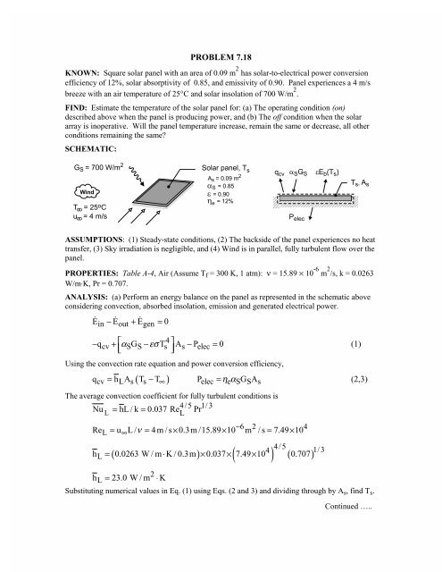
PROBLEM 7.18
KNOWN: Square solar panel with an area of 0.09 m 2 has solar-to-electrical power conversion
efficiency of 12%, solar absorptivity of 0.85, and emissivity of 0.90. Panel experiences a 4 m/s
breeze with an air temperature of 25°C and solar insolation of 700 W/m 2 .
FIND: Estimate the temperature of the solar panel for: (a) The operating condition (on)
described above when the panel is producing power, and (b) The off condition when the solar
array is inoperative. Will the panel temperature increase, remain the same or decrease, all other
conditions remaining the same
SCHEMATIC:
ASSUMPTIONS: (1) Steady-state conditions, (2) The backside of the panel experiences no heat
transfer, (3) Sky irradiation is negligible, and (4) Wind is in parallel, fully turbulent flow over the
panel.
PROPERTIES: Table A-4, Air (Assume T f = 300 K, 1 atm): ν = 15.89 × 10 -6 m 2 /s, k = 0.0263
W/m⋅K, Pr = 0.707.
ANALYSIS: (a) Perform an energy balance on the panel as represented in the schematic above
considering convection, absorbed insolation, emission and generated electrical power.
E in − E out + E
gen = 0
4
− qcv + ⎡αSGS −εσT ⎤
s As − Pelec
= 0
⎢⎣
⎥⎦
Using the convection rate equation and power conversion efficiency,
( )
qcv = hLAs Ts − T∞
Pelec = ηα e SGSAs
(2,3)
The average convection coefficient for fully turbulent conditions is
Nu 4/5 1/3
L
= hL / k = 0.037 Re L
Pr
Re
6 2 4
L = u L / ν 4m / s 0.3m /15.89 10
−
∞ = × × m / s = 7.49×
10
4/5
1/3
h
4
L = ( 0.0263 W / m⋅ K / 0.3m) × 0.037× ( 7.49×
10 ) ( 0.707)
h
2
L = 23.0 W / m ⋅K
Substituting numerical values in Eq. (1) using Eqs. (2 and 3) and dividing through by A s , find T s .
(1)
Continued …..

PROBLEM 7.18 (Cont.)
23 W / m
2
⋅K 2 8 2 4 4
( Ts
− 298)
K + 0.85× 700 W / m − 0.90× 5.67× 10
−
W / m ⋅K Ts
− 0.12 ⎡0.85 700 W / m
2 ⎤
⎢
×
⎥
= 0
(4)
⎣
⎦
Ts
= 302.2 K = 29.2° C
<
(b) If the solar array becomes inoperable (off) for reason of wire bond failures or the electrical
circuit to the battery is opened, the P elec term in the energy balance of Eq. (1) is zero. Using Eq.
(4) with η e = 0, find
Ts
= 31.7° C
<
COMMENTS: (1) Note how the electrical power P elec is represented by the E gen term in the
energy balance. Recall from Section 1.2 that E gen is associated with conversion from some form
of energy to thermal energy. Hence, the solar-to-electrical power conversion (P elec ) will have a
negative sign in Eq. (1).
(2) It follows that when the solar array is on, a fraction (η e ) of the absorbed solar power (thermal
energy) is converted to electrical energy. As such, the array surface temperature will be higher in
the off condition than in the on condition.
(3) Note that the assumed value for T f at which to evaluate the properties was reasonable.

PROBLEM 7.21
KNOWN: Surface characteristics of a flat plate in an air stream.
FIND: Orientation which minimizes convection heat transfer.
SCHEMATIC:
ASSUMPTIONS: (1) Surface B is sufficiently rough to trip the boundary layer when in the
upstream position (Configuration 2).
PROPERTIES: Table A-4, Air (T f = 333K, 1 atm): ν = 19.2 × 10 -6 m 2 /s, k = 28.7 × 10 -3
W/m⋅K, Pr = 0.7.
ANALYSIS: Since Configuration (2) results in a turbulent boundary layer over the entire surface,
the lowest heat transfer is associated with Configuration (1). Find
u L 20 m/s 1m
Re ∞ ×
6
L = = = 1.04×
10 .
ν 19.2×
10
-6
m
2
/s
Hence in Configuration (1), transition will occur just before the rough surface (x c = 0.48m). Note
that
4/5
( )
6
( ) ( )
⎡
6 ⎤
Nu
1/3
L,1
= ⎢0.037 1.04× 10 − 871 ⎥ 0.7 = 1366
⎣
⎦
4/5 1/3
NuL,2 = 0.037 1.04× 10 0.7 = 2139>
Nu
L,1.
hL,1L For Configuration (1): = Nu
L,1
= 1366.
k
Hence
and
−
( )
h
3 2
L,1 = 1366 28.7× 10 W/m⋅ K /1m= 39.2 W/m ⋅K
2
q1 = hL,1A( Ts
− T∞
) = 39.2 W/m ⋅ K( 0.5m× 1m)( 100−20)
K
q1
= 1568 W.

PROBLEM 7.33
KNOWN: Air at 27°C with velocity of 10 m/s flows turbulently over a series of electronic devices, each
having dimensions of 4 mm × 4 mm and dissipating 40 mW.
FIND: (a) Surface temperature T s of the fourth device located 15 mm from the leading edge, (b)
Compute and plot the surface temperatures of the first four devices for the range 5 ≤ u ∞ ≤ 15 m/s, and
(c) Minimum free stream velocity u ∞ if the surface temperature of the hottest device is not to exceed
80°C.
SCHEMATIC:
ASSUMPTIONS: (1) Turbulent flow, (2) Heat from devices leaving through top surface by convection
only, (3) Device surface is isothermal, and (4) The average coefficient for the devices is equal to the local
value at the mid position, i.e. h4 = hx(L).
T= Ts
+ T∞
2 = 315 K, 1 atm): k = 0.0274
W/m⋅K, ν = 17.40 × 10 -6 m 2 /s, α = 24.7 × 10 -6 m 2 /s, Pr = 0.705.
PROPERTIES: Table A.4, Air (assume T s = 330 K, ( )
ANALYSIS: (a) From Newton’s law of cooling,
Ts = T∞
+ qconv h4As
(1)
where h 4 is the average heat transfer coefficient over the 4th device. Since flow is turbulent, it is
reasonable and convenient to assume that
h4 = hx( L= 15mm)
. (2)
To estimate h x , use the turbulent correlation evaluating thermophysical properties at T f = 315 K (assume
T s = 330 K),
Nu
4/5 1/3
x = 0.0296 Rex
Pr
where
u L 10 m s 0.015m
Re ∞ ×
x = = = 8621
ν 17.4×
10
−6 m
2
s
giving
hxL
4/5 1/3
Nux
= = 0.0296( 8621) ( 0.705)
= 37.1
k
Nuxk
37.1× 0.0274 W m ⋅K
h
2
4 = hx
= = = 67.8 W m ⋅K
L 0.015m
Hence, with A s = 4 mm × 4 mm, the surface temperature is
40×
10
−3
W
$
Ts = 300 K + = 337 K = 64 C . <
2 3
2
67.8 W m ⋅ K × 4×
10
−
m
( )
Continued...

PROBLEM 7.33 (Cont.)
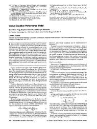
(b) The surface temperature for each of the four devices (i = 1, 2, 3 4) follows from Eq. (1),
Ts,i = T∞
+ qconv hi As
(3)
For devices 2, 3 and 4, h i is evaluated as the local coefficient at the mid-positions, Eq. (2), x 2 = 6.5 mm,
x 3 = 10.75 mm and x 4 = 15 mm. For device 1, h 1 is the average value 0 to x 1, where evaluated x 1 = L 1 =
4.25 mm. Using Eq. (3) in the IHT Workspace along with the Correlations Tool, External Flow, Local
Coefficient for Laminar or Turbulent Flow, the surface temperatures T s,i are determined as a function of
the free stream velocity.
100
Surface temperature, Ts (C)
90
80
70
60
50
40
5 7 9 11 13 15
Free stream velocity, uinf (m/s)
Device 1
Device 2
Device 3
Device 4
(c) Using the Explore option on the Plot Window associated with the IHT code of part (b), the minimum
free stream velocity of
u ∞ = 6.6 m/s <
will maintain device 4, the hottest of the devices, at a temperature T s,4 = 80°C.
COMMENTS: (1) Note that the thermophysical properties were evaluated at a reasonable assumed film
temperature in part (a).
(2) From the T s,i vs. u ∞ plots, note that, as expected, the surface temperatures of the devices increase with
distance from the leading edge.

PROBLEM 7.45
KNOWN: Pin fin of 10 mm diameter dissipates 30 W by forced convection in cross-flow of air with
ReD = 4000.
FIND: Fin heat rate if diameter is doubled while all conditions remain the same.
SCHEMATIC:
ASSUMPTIONS: (1) Pin behaves as infinitely long fin, (2) Conditions of flow, as well as base and
air temperatures, remain the same for both situations, (3) Negligible radiation heat transfer.
ANALYSIS: For an infinitely long pin fin, the fin heat rate is
( ) 1/2
qf = qconv = hPkAc θ b
where P = πD and A c = πD 2 /4. Hence,
( ⋅ ⋅
2) 1/2
q conv ~ h D D .
For forced convection cross-flow over a cylinder, an appropriate correlation for estimating the
dependence of h on the diameter is
m
hD m 1/3 ⎛VD
⎞
Nu
1/3
D
= = CRe
D
Pr = C Pr .
k
⎜
ν ⎟
⎝ ⎠
From Table 7.2 for Re D = 4000, find m = 0.466 and
It follows that
h~D
−1 D = D
−0.534
.
( ) 0.466
−
( ) 1/2
q
0.534 2 1.23
conv ~ D ⋅D⋅ D = D .
Hence, with q 1 → D 1 (10 mm) and q 2 → D 2 (20 mm), find
1.23 1.23
⎛D2
⎞ ⎛20
⎞
q2 = q1⎜ ⎟ = 30 W = 70.4 W.
D
⎜
1
10
⎟
⎝ ⎠ ⎝ ⎠
COMMENTS: The effect of doubling the diameter, with all other conditions remaining the same, is
to increase the fin heat rate by a factor of 2.35. The effect is nearly linear, with enhancements due to
the increase in surface and cross-sectional areas (D 1.5 ) exceeding the attenuation due to a decrease in
the heat transfer coefficient (D -0.267 ). Note that, with increasing Reynolds number, the exponent m
increases and there is greater heat transfer enhancement due to increasing the diameter.

PROBLEM 7.62
KNOWN: Long coated plastic, 20-mm diameter rod, initially at a uniform temperature of T i = 25°C, is
suddenly exposed to the cross-flow of air at T ∞ = 350°C and V = 50 m/s.
FIND: (a) Time for the surface of the rod to reach 175°C, the temperature above which the special
coating cures, and (b) Compute and plot the time-to-reach 175°C as a function of air velocity for 5 ≤ V ≤
50 m/s.
SCHEMATIC:
ASSUMPTIONS: (a) One-dimensional, transient conduction in the rod, (2) Constant properties, and (3)
Evaluate thermophysical properties at T f = [(T s + T i )/2 + T ∞ ] = [(175 + 25)/2 + 350]°C = 225°C = 500 K.
PROPERTIES: Rod (Given): ρ = 2200 kg/m 3 , c = 800 J/kg⋅K, k = 1 W/m⋅K, α = k/ρc = 5.68 × 10 -7
m 2 /s; Table A.4, Air (T f ≈ 500 K, 1 atm): ν = 38.79 × 10 -6 m 2 /s, k = 0.0407 W/m⋅K, Pr = 0.684.
ANALYSIS: (a) To determine whether the lumped capacitance method is valid, determine the Biot
number
h( ro
2)
Bilc
= (1)
k
The convection coefficient can be estimated using the Churchill-Bernstein correlation, Eq. 7.57,
4/5
1/2 1/3
5/8
hD 0.63ReD
Pr ⎡
⎛ ReD
⎞
⎤
NuD
= = 0.3 + ⎢1
+
k 2/3
1/4 ⎜ ⎟ ⎥
⎡ ⎢ ⎝282,000
⎠ ⎥
1+
( 0.4 Pr)
⎤ ⎣ ⎦
⎢⎣
⎥⎦
Re VD
6 2
D = = 50 m s× 0.020 m 38.79× 10
−
m s = 25,780
ν
⎧
4/5⎫
1/2 1/3
5/8
⎪ 0.63( 25, 780) ( 0.684)
⎡ ⎛ ⎞ ⎤ ⎪
⎨
⎢
1/4
⎜ ⎟ ⎥ ⎬
⎪ ⎡ 2/3 ⎝ ⎠
1+
( 0.4 0.684)
⎤ ⎢⎣ ⎥⎦
⎪
⎩ ⎣ ⎦ ⎭
0.0407 W m ⋅ K 25, 780
h = 0.3+ 1+
0.020 m 282, 000
= 184 W/m 2 ⋅K(2)
Substituting for h from Eq. (2) into Eq. (1), find
Bi
2
lc = 184 W m ⋅K( 0.010 m 2)
1W m⋅ K = 0.92 >> 0.1
Hence, the lumped capacitance method is inappropriate. Using the one-term series approximation,
Section 5.6.2, Eqs. 5.49 with Table 5.1,
θ
*
= C
2 * *
1exp − ζ
1
Fo Jo ζ1r r = r ro
= 1
( ) ( )
( o ) − ∞ ( − )
i − ∞ ( −
$
)
* T r , t T 175 350 C
θ = = = 0.54
T T 25 350 C
$
Bi = hro k = 1.84 ζ1= 1.5308 rad C1=
1.3384
Continued...

PROBLEM 7.62 (Cont.)
0.54 = 1.3384exp[-(1.5308rad) 2 Fo]J o (1.5308 × 1)
Using Table B.4 to evaluate J o (1.5308) = 0.4944, find Fo = 0.0863 where
αt 7 2
o 5.68× 10
−
m s×
t
Fo = = o = 5.68× 10
−3
t
2 2
o
ro
( 0.010 m)
(6)
to
= 15.2s
<
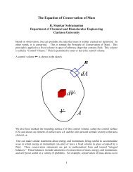
(b) Using the IHT Model, Transient Conduction, Cylinder, and the Tool, Correlations, External Flow,
Cylinder, results for the time-to-reach a surface temperature of 175°C as a function of air velocity V are
plotted below.
100
80
Time, to (s)
60
40
20
0
0 10 20 30 40 50
Air velocity, V (m/s)
COMMENTS: (1) Using the IHT Tool, Correlations, External Flow, Cylinder, the effect of the film
temperature T f on the estimated convection coefficient with V = 50 m/s can be readily evaluated.
T f (K) 460 500 623
h (W/m 2 ⋅K) 187 184 176
At early times, h = 184 W/m 2 ⋅K is a good estimate, while as the cylinder temperature approaches the
airsteam temperature, the effect starts to be noticeable (10% decrease).
(2) The IHT analysis performed for part (b) was developed in two parts. Using a known value for h , the
Transient Conduction, Cylinder Model was tested. Separately, the Correlation Tools was assembled and
tested. Then, the two files were merged to give the workspace for determining the time-to-reach 175°C
as a function of velocity V.

PROBLEM 7.65
KNOWN: Temperature and velocity of water flowing over a sphere of prescribed temperature and
diameter.
FIND: (a) Drag force, (b) Rate of heat transfer.
SCHEMATIC:
ASSUMPTIONS: (1) Steady-state conditions, (2) Uniform surface temperature.
PROPERTIES: Table A-6, Saturated Water (T ∞ = 293K): ρ = 998 kg/m 3 , µ = 1007 × 10 -6 N⋅s/m 2 ,
k = 0.603 W/m⋅K, Pr = 7.00; (T s = 333 K): µ = 467 × 10 -6 N⋅s/m 2 ; (T f = 313 K): ρ = 992 kg/m 3 , µ =
657 × 10 -6 N⋅s/m 2 .
ANALYSIS: (a) Evaluating µ and ρ at the film temperature,
ρVD
( 992 kg/m 3 ) 5 m/s ( 0.02 m)
Re
5
D = = = 1.51×
10
µ 657× 10
-6
Ns/m ⋅
2
and from Fig. 7.8, C D = 0.42. Hence
π D
2
V
2 π ( 0.02 m) 2 kg ( 5 m/s )
2
FD = CD ρ = 0.42 992 = 1.64 N. <
4 2 4 m
3 2
(b) With the Reynolds number evaluated at the free stream temperature,
3
ρVD
998 kg/m ( 5 m/s ) ( 0.02 m)
Re
4
D = = = 9.91×
10
µ 1007× 10
-6
Ns/m ⋅
2
it follows from the Whitaker relation that
1/4
1/2 2/3 0.4 ⎛ µ ⎞
NuD
= 2+ ⎡0.4ReD
0.06Re ⎤
⎢
+ D Pr
⎣ ⎥⎦ ⎜ ⎟
⎝µ
s ⎠
⎡ 1/4
4
1/2
4
2/3⎤ 0.4⎛1007
⎞
NuD
= 2+ ⎢0.4( 9.91× 10 ) + 0.06( 9.91× 10 ) ⎥( 7.0)
⎜ = 673.
467
⎟
⎣
⎦ ⎝ ⎠
Hence, the convection coefficient and heat rate are
k 0.603 W/m⋅K
h = Nu
2
D
= 673= 20,300 W/m ⋅K
D 0.02 m
2
W
2 o
q = h( πD ) ( Ts − T∞
) = 20,300 π ( 0.02 m ) ( 60− 20)
C=
1020 W. <
m
2
⋅ K
COMMENTS: Compare the foregoing value of h with that obtained in the text example under
similar conditions. The significant increase in h is due to the much larger value of k and smaller value
of ν for the water. Note that Re D is slightly beyond the range of the correlation.

PROBLEM 7.78
KNOWN: Velocity and temperature of combustion gases. Diameter and emissivity of thermocouple
junction. Combustor temperature.
FIND: (a) Time to achieve 98% of maximum thermocouple temperature rise, (b) Steady-state
thermocouple temperature, (c) Effect of gas velocity and thermocouple emissivity on measurement error.
SCHEMATIC:
ASSUMPTIONS: (1) Validity of lumped capacitance analysis, (2) Constant properties, (3) Negligible
conduction through lead wires, (4) Radiation exchange between small surface and a large enclosure
(parts b and c).
PROPERTIES: Thermocouple (given): 0.1 ≤ ε ≤ 1.0, k = 100 W/m⋅K, c = 385 J/kg⋅K, ρ = 8920 kg/m 3 ;
Gases (given): k = 0.05 W/m⋅K, ν = 50 × 10 -6 m 2 /s, Pr = 0.69.
ANALYSIS: (a) If the lumped capacitance analysis may be used, it follows from Equation 5.5 that
ρVc Ti
− T Dρc
t = ln ∞ = ln( 50)
.
hAs
T − T∞
6h
Neglecting the viscosity ratio correlation for variable property effects, use of V = 5 m/s with the
Whitaker correlation yields
1/2 2/3 0.4
VD 5 m s( 0.001m)
NuD = ( hD k) = 2 + ( 0.4 ReD + 0.06 ReD ) Pr ReD = = = 100
ν
−6 2
50×
10 m s
0.05W m ⋅K
h =
⎡
2 + ( 0.4( 100) 1/2 + 0.06( 100)
2/3 )( 0.69)
0.4 ⎤
= 328W m 2 ⋅K
0.001m ⎢⎣
⎥⎦
Since Bi = h( ro
3)
k = 5.5 × 10 -4 , the lumped capacitance method may be used. Hence,
3
( )
0.001m 8920 kg m 385J kg ⋅K
t = ln ( 50)
= 6.83s
6× 328 W m
2
⋅K
(b) Performing an energy balance on the junction and evaluating radiation exchange from Equation 1.7,
q conv = q rad . Hence, with ε = 0.5,
hA
4 4
s T∞ − T = εAsσ
T −Tc
( ) ( )
0.5× 5.67× 10
−8 W m
2
⋅K
4
4 4 4
( 1000 − T) K = ⎡T −( 400)
⎤K
.
328W m
2
⋅ K
⎢⎣
⎥⎦
T = 936 K <
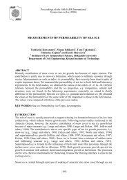
(c) Using the IHT First Law Model for a Solid Sphere with the appropriate Correlation for external flow
from the Tool Pad, parametric calculations were performed to determine the effects of V and ε g , and the
following results were obtained.
Continued...

PROBLEM 7.78 (Cont.)
1000
990
Temperature, T(K)
950
Temperature, T(K)
970
950
930
910
900
0 5 10 15 20 25
Velocity, V(m/s)
Emissivity, epsilon = 0.5
890
0.1 0.2 0.3 0.4 0.5 0.6 0.7 0.8 0.9 1
Emissivity
Velocity, V = 5 m/s
Since the temperature recorded by the thermocouple junction increases with increasing V and decreasing
ε, the measurement error, T ∞ - T, decreases with increasing V and decreasing ε. The error is due to net
radiative transfer from the junction (which depresses T) and hence should decrease with decreasing ε.
For a prescribed heat loss, the temperature difference ( T ∞ - T) decreases with decreasing convection
resistance, and hence with increasing h(V).
COMMENTS: To infer the actual gas temperature (1000 K) from the measured result (936 K),
correction would have to be made for radiation exchange with the cold surroundings.