Chapter 17 Radio Propagation Models
Chapter 17 Radio Propagation Models
Chapter 17 Radio Propagation Models

You also want an ePaper? Increase the reach of your titles
YUMPU automatically turns print PDFs into web optimized ePapers that Google loves.
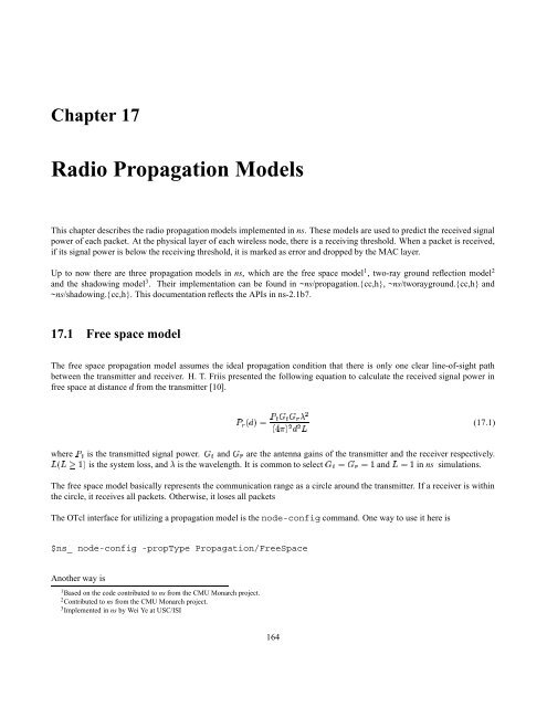
<strong>Chapter</strong> <strong>17</strong><br />
<strong>Radio</strong> <strong>Propagation</strong> <strong>Models</strong><br />
This chapter describes the radio propagation models implemented in ns. These models are used to predict the received signal<br />
power of each packet. At the physical layer of each wireless node, there is a receiving threshold. When a packet is received,<br />
if its signal power is below the receiving threshold, it is marked as error and dropped by the MAC layer.<br />
Up to now there are three propagation models in ns, which are the free space model 1 , two-ray ground reflection model 2<br />
and the shadowing model 3 . Their implementation can be found in ~ns/propagation.{cc,h}, ~ns/tworayground.{cc,h} and<br />
~ns/shadowing.{cc,h}. This documentation reflects the APIs in ns-2.1b7.<br />
<strong>17</strong>.1 Free space model<br />
The free space propagation model assumes the ideal propagation condition that there is only one clear line-of-sight path<br />
between the transmitter and receiver. H. T. Friis presented the following equation to calculate the received signal power in<br />
free space at distance from the transmitter [10].<br />
¢ ¡£<br />
¦ (<strong>17</strong>.1)<br />
¤¥<br />
¡£¢¥¤ §¦©¨<br />
where is the transmitted signal power. and are the antenna gains of the transmitter and the receiver respectively.<br />
¢ ¡£ ¤ ¦ <br />
is the system loss, and is the wavelength. It is common to select and in ns simulations.<br />
¨ ¢¨ ¨ <br />
The free space model basically represents the communication range as a circle around the transmitter. If a receiver is within<br />
the circle, it receives all packets. Otherwise, it loses all packets<br />
The OTcl interface for utilizing a propagation model is the node-config command. One way to use it here is<br />
$ns_ node-config -propType <strong>Propagation</strong>/FreeSpace<br />
Another way is<br />
1 Based on the code contributed to ns from the CMU Monarch project.<br />
2 Contributed to ns from the CMU Monarch project.<br />
3 Implemented in ns by Wei Ye at USC/ISI<br />
164
set prop [new <strong>Propagation</strong>/FreeSpace]<br />
$ns_ node-config -propInstance $prop<br />
<strong>17</strong>.2 Two-ray ground reflection model<br />
A single line-of-sight path between two mobile nodes is seldom the only means of propation. The two-ray ground reflection<br />
model considers both the direct path and a ground reflection path. It is shown [20] that this model gives more accurate<br />
prediction at a long distance than the free space model. The received power at distance is predicted by<br />
¢¡ ¢ <br />
¡£<br />
(<strong>17</strong>.2)<br />
£¢<br />
¡£¢¥¤ §¦©¨<br />
¢<br />
. ¨ where and are the heights of the transmit and receive antennas respectively. Note that the original equation in [20]<br />
assumes To be consistent with the free space model, is added here.<br />
The above equation shows a faster power loss than Eqn. (<strong>17</strong>.1) as distance increases. However, The two-ray model does not<br />
give a good result for a short distance due to the oscillation caused by the constructive and destructive combination of the two<br />
rays. Instead, the free space model is still used when is small.<br />
Therefore, a cross-over distance ¥¤ is calculated in this model. When §¦ ¥¤ , Eqn. (<strong>17</strong>.1) is used. When §¨ ©¤ , Eqn. (<strong>17</strong>.2)<br />
is used. At the cross-over distance, Eqns. (<strong>17</strong>.1) and (<strong>17</strong>.2) give the same result. So ¤ can be calculated as<br />
¤ ¨ ¤ ¥ ¢ ¦ <br />
(<strong>17</strong>.3)<br />
Similarly, the OTcl interface for utilizing the two-ray ground reflection model is as follows.<br />
$ns_ node-config -propType <strong>Propagation</strong>/TwoRayGround<br />
Alternatively, the user can use<br />
set prop [new <strong>Propagation</strong>/TwoRayGround]<br />
$ns_ node-config -propInstance $prop<br />
<strong>17</strong>.3 Shadowing model<br />
<strong>17</strong>.3.1 Backgroud<br />
The free space model and the two-ray model predict the received power as a deterministic function of distance. They both<br />
represent the communication range as an ideal circle. In reality, the received power at certain distance is a random variable<br />
due to multipath propagation effects, which is also known as fading effects. In fact, the above two models predicts the mean<br />
received power at distance . A more general and widely-used model is called the shadowing model [20].<br />
165
¡<br />
Table <strong>17</strong>.1: Some typical values of path loss exponent ¡<br />
Table <strong>17</strong>.2: Some typical values of shadowing deviation §©¨<br />
¡ ¢ ¤ ¦ <br />
¤ ¦ ¡£¢<br />
¡ ¢ ¤ ¦ %<br />
¦'& ¡£¢¥¤<br />
<br />
<br />
Environment<br />
Outdoor Free space 2<br />
Shadowed urban area 2.7 to 5<br />
In building Line-of-sight 1.6 to 1.8<br />
Obstructed 4 to 6<br />
Environment<br />
Outdoor 4 to 12<br />
¢¤£¦¥ (dB)<br />
Office, hard partition 7<br />
Office, soft partition 9.6<br />
Factory, line-of-sight 3 to 6<br />
Factory, obstructed 6.8<br />
The shadowing model consists of two parts. The first one is known as path loss model, which also predicts the mean received<br />
power at distance , denoted by . It uses a close-in distance as a reference. is computed relative to as<br />
¢ ¤ §¦ ¡ ¢ ¤ ¦<br />
follows.<br />
¡ §¦ ¤ ¢ ¡<br />
¡£¢¥¤ ¦<br />
(<strong>17</strong>.4)<br />
¨<br />
¡ ¢ ¤ §¦<br />
is called the path loss exponent, and is usually empirically determined by field measurement. From Eqn.<br />
¨<br />
¡ (<strong>17</strong>.1) we know that<br />
for free space propagation. Table <strong>17</strong>.1 ¡ gives some typical values of . Larger values correspond to more obstructions<br />
and hence faster decrease in average received power as distance becomes larger. can be computed from Eqn. (<strong>17</strong>.1).<br />
¦ ¤ ¢ ¡<br />
The path loss is usually measured in dB. So from Eqn. (<strong>17</strong>.4) we have<br />
$ (<strong>17</strong>.5)<br />
¨ <br />
¡! #"<br />
¨<br />
The second part of the shadowing model reflects the variation of the received power at certain distance. It is a log-normal<br />
random variable, that is, it is of Gaussian distribution if measured in dB. The overall shadowing model is represented by<br />
*),+ ¨ (<strong>17</strong>.6)<br />
¨( <br />
¡! #"<br />
¨<br />
where + ¨ is a Gaussian random variable with zero mean and standard deviation § ¨ . § ¨ is called the shadowing deviation,<br />
and is also obtained by measurement. Table <strong>17</strong>.2 shows some typical values of § ¨ . Eqn. (<strong>17</strong>.6) is also known as a log-normal<br />
shadowing model.<br />
The shadowing model extends the ideal circle model to a richer statistic model: nodes can only probabilistically communicate<br />
when near the edge of the communication range.<br />
166
<strong>17</strong>.3.2 Using shadowing model<br />
Before using the model, the user should select the values of the path loss ¡ exponent<br />
according to the simulated environment.<br />
and the shadowing deviation § ¨<br />
The OTcl interface is still the node-config command. One way to use it is as follows, and the values for these parameters<br />
are just examples.<br />
# first set values of shadowing model<br />
<strong>Propagation</strong>/Shadowing set pathlossExp_ 2.0<br />
<strong>Propagation</strong>/Shadowing set std_db_ 4.0<br />
<strong>Propagation</strong>/Shadowing set dist0_ 1.0<br />
<strong>Propagation</strong>/Shadowing set seed_ 0<br />
;# path loss exponent<br />
;# shadowing deviation (dB)<br />
;# reference distance (m)<br />
;# seed for RNG<br />
$ns_ node-config -propType <strong>Propagation</strong>/Shadowing<br />
The shadowing model creates a random number generator (RNG) object. The RNG has three types of seeds: raw seed,<br />
pre-defined seed (a set of known good seeds) and the huristic seed (details in Section 20.1). The above API only uses the<br />
pre-defined seed. If a user want different seeding method, the following API can be used.<br />
set prop [new <strong>Propagation</strong>/Shadowing]<br />
$prop set pathlossExp_ 2.0<br />
$prop set std_db_ 4.0<br />
$prop set dist0_ 1.0<br />
$prop seed 0<br />
;# user can specify seeding method<br />
$ns_ node-config -propInstance $prop<br />
The above can be raw, predef or heuristic.<br />
<strong>17</strong>.4 Communication range<br />
In some applications, a user may want to specify the communication range of wireless nodes. This can be done by set an<br />
appropriate value of the receiving threshold in the network interface, i.e.,<br />
Phy/WirelessPhy set RXThresh_ <br />
A separate C program is provided at ~ns/indep-utils/propagation/threshold.cc to compute the receiving threshold. It can be<br />
used for all the propagation models discussed in this chapter. Assume you have compiled it and get the excutable named as<br />
threshold. You can use it to compute the threshold as follows<br />
threshold -m [other-options] distance<br />
where is either FreeSpace, TwoRayGround or Shadowing, and the distance is the<br />
communication range in meter.<br />
167
[other-options] are used to specify parameters other than their default values. For the shadowing model there is a<br />
necessary parameter, -r , which specifies the rate of correct reception at the distance. Because<br />
the communication range in the shadowing model is not an ideal circle, an inverse Q-function [20] is used to calculate the<br />
receiving threshold. For example, if you want 95% of packets can be correctly received at the distance of 50m, you can<br />
compute the threshold by<br />
threshold -m Shadowing -r 0.95 50<br />
Other available values of [other-options] are shown below<br />
-pl -std -Pt <br />
-fr -Gt -Gr <br />
-L -ht -hr <br />
-d0 <br />
<strong>17</strong>.5 Commands at a glance<br />
Following is a list of commands for propagation models.<br />
$ns_ node-config -propType <br />
This command selects in the simulation. the can be<br />
<strong>Propagation</strong>/FreeSpace, <strong>Propagation</strong>/TwoRayGround or <strong>Propagation</strong>/Shadowing<br />
$ns_ node-config -propInstance $prop<br />
This command is another way to utilize a propagation model. $prop is an instance of the .<br />
$sprop_ seed <br />
This command seeds the RNG. $sprop_ is an instance of the shadowing model.<br />
threshold -m [other-options] distance<br />
This is a separate program at ~ns/indep-utils/propagation/threshold.cc, which is used to compute the receiving threshold for<br />
a specified communication range.<br />
168
![Problem 1: Loop Unrolling [18 points] In this problem, we will use the ...](https://img.yumpu.com/36629594/1/184x260/problem-1-loop-unrolling-18-points-in-this-problem-we-will-use-the-.jpg?quality=85)