Theory of General Competitive Equilibrium and Optimization Models ...
Theory of General Competitive Equilibrium and Optimization Models ...
Theory of General Competitive Equilibrium and Optimization Models ...

You also want an ePaper? Increase the reach of your titles
YUMPU automatically turns print PDFs into web optimized ePapers that Google loves.
N<br />
PCC B<br />
H<br />
X<br />
OB<br />
Y<br />
N<br />
I x1<br />
I x2<br />
I x3<br />
I x4<br />
L<br />
O Y<br />
K<br />
Y<br />
O A<br />
X<br />
G<br />
Figure 5.<br />
E<br />
PCC A<br />
B e<br />
A e<br />
K<br />
O X<br />
L<br />
F<br />
E<br />
G<br />
I y1<br />
I y4 Iy3<br />
I y2<br />
Figure 6.<br />
We can see the point <strong>of</strong> section <strong>of</strong> supply curves <strong>of</strong><br />
observed traders <strong>of</strong> exchange is on Edgeworth contract<br />
curve <strong>and</strong> inside <strong>of</strong> the core <strong>of</strong> exchange in the interval <strong>of</strong><br />
points G <strong>and</strong> H in point E. It expresses the relations <strong>of</strong><br />
exchange where the product <strong>of</strong>fer <strong>of</strong> the individual A (i.e.<br />
his dem<strong>and</strong> for product Y) <strong>and</strong> product <strong>of</strong>fer by trader B<br />
(i.e. his dem<strong>and</strong> for product X). The general exchange<br />
equilibrium is established in point E – <strong>of</strong> course, in the<br />
simplified model with two traders <strong>and</strong> two products.<br />
However, this model enables to define the general law on<br />
equilibrium <strong>of</strong> exchange in the following sense: general<br />
exchange equilibrium is established with equality <strong>of</strong><br />
marginal substitution rates <strong>of</strong> traders along with equality<br />
<strong>of</strong> supply <strong>and</strong> dem<strong>and</strong> that they present.<br />
The analysis <strong>of</strong> general equilibrium mechanism is<br />
needed to continue by researching the mechanism <strong>of</strong><br />
general production equilibrium.<br />
III. GENERAL PRODUCTION EQUILIBRIUM<br />
In analyzing <strong>of</strong> general production equilibrium, we can<br />
take the simplified production model analog to the model<br />
used in the analysis <strong>of</strong> general exchange equilibrium. In<br />
the model, we suppose that a producer makes two<br />
products X <strong>and</strong> Y, with combination <strong>of</strong> only two inputs,<br />
labor <strong>and</strong> capital, i.e. by means <strong>of</strong> L (Labor) <strong>and</strong> C<br />
(Capital). The general production equilibrium is<br />
established when marginal technical rate <strong>of</strong> factor<br />
substitution equalize, i.e. MRTS (Marginal Rate <strong>of</strong><br />
Technical Substitution) for both products. <strong>Equilibrium</strong><br />
can be established on the so-called Edgeworth closed<br />
production box [Kopanyi, 2003], i.e. in Figure 6. The<br />
curves IX1, IX2, IX3 <strong>and</strong> IX4 represent isoquants or the<br />
so-called curves <strong>of</strong> equal product <strong>of</strong> production <strong>of</strong> product<br />
X. Therefore, isoquants IY1, IY2, IY3 <strong>and</strong> IY4 show the<br />
curves <strong>of</strong> equal products for product Y. If the starting<br />
point is point N in the section <strong>of</strong> isoquants IX1 <strong>and</strong> IY3, it<br />
is visible that production maximization X <strong>and</strong> Y is not<br />
realized here, therefore, nor general production<br />
equilibrium. The producer can increase both production X<br />
<strong>and</strong> production Y, i.e. reaches isoquants at the higher<br />
position (i.e. further than the origo) reducing capital<br />
consumption for production X on behalf <strong>of</strong> production Y<br />
<strong>and</strong> conversely, increasing labor consumption in<br />
production X, on behalf <strong>of</strong> consumed labor in production<br />
Y.<br />
With these relations <strong>and</strong> limitations, production<br />
maximization <strong>of</strong> both products is reached in the tangential<br />
point <strong>of</strong> production isoquants X <strong>and</strong> Y, i.e. at point E. In<br />
point E, the curve slopes <strong>of</strong> equal products X <strong>and</strong> Y, i.e.<br />
Ix2 <strong>and</strong> Iy3 are equal, i.e. the marginal technical rates <strong>of</strong><br />
substitution in their production are equalized. Thence,<br />
these relations are valid:<br />
MRTS = MRTS Then (5)<br />
L, K(X)<br />
MP<br />
MRTS L,K =<br />
MP<br />
L<br />
K<br />
L, K(Y)<br />
(MP=Marginal Product) (6)<br />
;<br />
It means that production equilibrium criterion is realized<br />
with the condition<br />
⎛ MPL<br />
⎞ ⎛ MPL<br />
⎞<br />
⎜<br />
MP<br />
⎟ =<br />
⎜<br />
K MP<br />
⎟<br />
⎝ ⎠X<br />
⎝ K ⎠Y<br />
(7)<br />
The point <strong>of</strong> equilibrium is on the so-called Edgewort<br />
contract production curve, which connects origo Ox <strong>and</strong><br />
origo Oy. When production <strong>of</strong> goods is on this curve, it is<br />
not possible any more to increase production <strong>of</strong> one<br />
material product without decreasing production <strong>of</strong> the<br />
other product. On the contract production curve, there are<br />
such combinations <strong>of</strong> production <strong>of</strong> goods, which realize<br />
the so-called Pareto production equilibrium [Pareto,<br />
1971]. In the above analysis <strong>of</strong> production equilibrium,<br />
two marginal rates <strong>of</strong> technical substitution <strong>and</strong> marginal<br />
products <strong>of</strong> observed are taken into consideration, but not<br />
using the price factor.<br />
In further analysis, suppose that the sum <strong>of</strong> engaged<br />
resources (or TC – total costs) is the constant for<br />
production <strong>of</strong> goods X <strong>and</strong> Y. Then, suppose that, with<br />
ceteris paribus, labor price, i.e. PL1 < PL2 < PL3 in<br />
production <strong>of</strong> product X decreases gradually. So, we<br />
obtain isocost lines (lines <strong>of</strong> equal costs) in different<br />
positions for production <strong>of</strong> product X. Connecting<br />
tangential points <strong>of</strong> appropriate isoquants <strong>and</strong> isocost lines<br />
with different labor prices, we obtain the production curve<br />
<strong>of</strong> product X, which expresses the optimal combination <strong>of</strong><br />
input under cited conditions, i.e. the curve Tx.