Energy dispersive X-ray fluorescence (EDXRF) for studying coinage ...
Energy dispersive X-ray fluorescence (EDXRF) for studying coinage ...
Energy dispersive X-ray fluorescence (EDXRF) for studying coinage ...

Create successful ePaper yourself
Turn your PDF publications into a flip-book with our unique Google optimized e-Paper software.
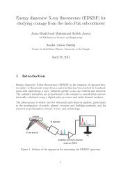
<strong>Energy</strong> <strong>dispersive</strong> X-<strong>ray</strong> <strong>fluorescence</strong> (<strong>EDXRF</strong>) <strong>for</strong><br />
<strong>studying</strong> <strong>coinage</strong> from the Indo-Pak subcontinent<br />
Asma Khalid and Muhammad Sabieh Anwar<br />
LUMS School of Science and Engineering<br />
Saadat Anwar Siddiqi<br />
Centre <strong>for</strong> Solid State Physics, University of the Punjab<br />
May 2, 2011<br />
1 Introduction<br />
<strong>Energy</strong> <strong>dispersive</strong> X-<strong>ray</strong> <strong>fluorescence</strong> (<strong>EDXRF</strong>) is the emission of characteristic,<br />
secondary or fluorescent X-<strong>ray</strong>s from a material that has been excited by bombardment<br />
with high-energy X-<strong>ray</strong>s. Element specific X-<strong>ray</strong>s are emitted and detected.<br />
The radiative intensities are proportional to the element’s concentration and are<br />
internally calculated using a digital pulse processor and multi channel analyzer.<br />
The phenomenon is widely used <strong>for</strong> elemental and chemical analysis, particularly<br />
in the investigation of metals, glasses, ceramics and building materials, and <strong>for</strong><br />
research in geochemistry, <strong>for</strong>ensic science and archaeology.<br />
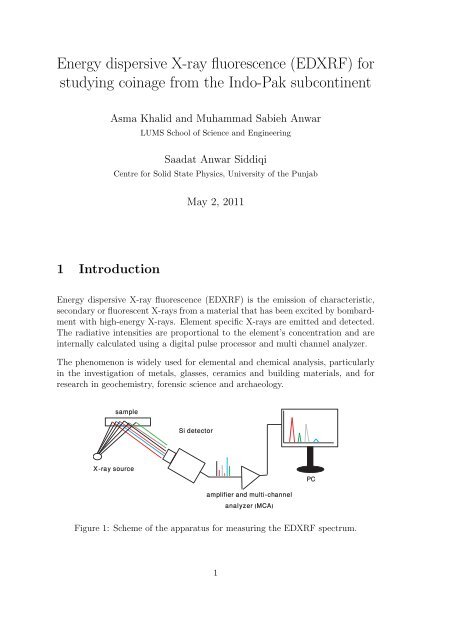
sample<br />
Si detector<br />
X-<strong>ray</strong> source<br />
amplifier and multi-channel<br />
analyzer (MCA)<br />
PC<br />
Figure 1: Scheme of the apparatus <strong>for</strong> measuring the <strong>EDXRF</strong> spectrum.<br />
1
2 Application of <strong>EDXRF</strong> in numismatics<br />
Coins are an important source of history. Numismatics is the study of coins that<br />
involves the analysis of the <strong>coinage</strong> materials, their metallic composition as well as<br />
the identification of the sources of the metals. On the basis of coin archeometry,<br />
we can classify coins on the basis of their fabric (size, shape, design, thickness<br />
and workmanship), metrology (weight), design, metallic composition, techniques<br />
of manufacturing and message content. Various analytical techniques are used <strong>for</strong><br />
ascertaining the metal content of coins [1].<br />
Coinage is interesting from the historic point of view because it helps learn facts<br />
about the past that are otherwise unknown. Coins are archaeological objects which<br />
have to be interpreted and studied to gain important historical in<strong>for</strong>mation. They<br />
supply us with in<strong>for</strong>mation about events long after their occurrence. They are also<br />
official emblems, and thus likely to provide accurate, reliable and authoritative<br />
in<strong>for</strong>mation about governments. Moreover, minting is one of the oldest <strong>for</strong>ms of<br />
mass production. Coins provide vital evidence about metallurgical history which<br />
has shaped the progress of civilizations [2].<br />
2.1 <strong>EDXRF</strong> and numismatics<br />
An important application of <strong>EDXRF</strong> is the characterization of coins. <strong>EDXRF</strong><br />
spectrometry is a non-destructive technique. The technique does not require special<br />
sample preparation. It is fast, non destructive, sensitive, and capable of multi<br />
elemental analysis [3, 4].<br />
Coins can be sources <strong>for</strong> the following valuable in<strong>for</strong>mation:<br />
1. coin minting methodologies,<br />
2. ores employed <strong>for</strong> coin minting,<br />
3. relative percentage of metals in coins of different reigns, regions, etc.,<br />
4. correlating variations in alloy composition with debasement of coins and thus<br />
the economic stability of an era or a political empire,<br />
5. distinguishing imitations from authentic coin specimens, and<br />
6. detection of trace element in coins.<br />
Some vital in<strong>for</strong>mation that can be gleaned from numismatic spectroscopy is highlighted<br />
below.<br />
2.2 Monetary and economic affluence<br />
In ancient times, the noble metal content of a coin was used to reflect its real<br />
value, so that the denomination of coins was directly related to the economic and<br />
2
political situation. The debasement of coins was indicative of normal inflation.<br />
The persistence of political instability, e.g., civil wars, often led to poorly minted<br />
coins. In turbulent times, the necessary ores or metals from mines did not reach the<br />
mint and substitute elements had to be used imparting an unusual concentration<br />
to the coins. Imitations were also made during all periods.<br />
For example, in the early medieval era (400 to 700 AD), there was a scarcity of<br />
<strong>coinage</strong> throughout north India which is an indicative of a low level of exchange<br />
transactions, and hence a quiescence of trade and commerce. Gold coins were<br />
rarely issued after the fall of the Gupta Empire (320 to 550 AD) and even the<br />
silver and copper coins were scarce and poorly minted. In contrast, during the<br />
economic expansion of the Mughal era (1556 to 1748 AD), the imperial reserves<br />
of precious metals and gems swelled, specially during Akbar’s reign (1556 to 1605<br />
AD) and the high quality and purity of metal was maintained in coins of gold,<br />
silver and copper. In the early Mughal period, whatever the available sources of<br />
gold and silver, India was the ultimate sink <strong>for</strong> these metals. Similarly, during the<br />
British rule in India, the price of silver skyrocketed after the outbreak of World<br />
War II in 1939 and the practice of hoarding silver coins became common. This led<br />
to reducing the use of silver in coins. Hence, the tracking of elemental compositions<br />
is one important indicator of monetary and political history.<br />
2.3 Production and manufacturing techniques<br />
The composition of coins has fluctuated widely in different time periods due to variation<br />
in production techniques. For example, the refinement of metals at the end<br />
of the seventeenth century has stamped its influence on the production techniques.<br />
Prior to 1700 AD, the coins of Cu and the noble metals Ag and Au contained<br />
additional elements and impurities such as Pb, Sn, Bi, Hg, but the coins produced<br />
at the end of the eighteenth century AD were found to have purity exceeding 99%.<br />
2.4 Relation to the ores and trace element detection<br />
The <strong>EDXRF</strong> of ancient coins can help identify the ore used in coins. The concentration<br />
of the chief element of the coin and the trace elements present in the<br />
coins provide important clues about the ore. The data can also be related to the<br />
manufacturing and minting techniques of that era. We can also predict whether<br />
the ore was mined near the mint or was traded and transported to the mint [5, 6].<br />
In short, the XRF study of sub-continent’s coins can provide useful in<strong>for</strong>mation<br />
of how the coins and the minting technology flourished over time, what changes<br />
were affected in the composition and texture of the coins, how the use of precious<br />
metals like gold and silver started <strong>for</strong> <strong>coinage</strong>, what were the sources of these<br />
metals in the subcontinent, what were the weight standards <strong>for</strong> different coins and<br />
why the weight percentage of precious metals fluctuated in different reigns and<br />
periods. The study can also help discover the methods of the extraction of <strong>coinage</strong><br />
elements (gold, silver and copper) from their respective ores and the history of<br />
3
different mines in the region as well as the tracing of mercantile and trade routes.<br />
3 Proposed experimental work on coin archeometry<br />
using <strong>EDXRF</strong><br />
The objective of the proposed experiment is to analyze and study the historical<br />
coins of the sub-continent that were minted in the region from approximately 200<br />
BC to 1947 AD. For this purpose, a collaboration with the Lahore museum would<br />
be beneficial since these museums possess a treasure of coins which were minted and<br />
used during different historical periods. The X-<strong>ray</strong> spectroscopy of the coins can<br />
provide a good opportunity to understand the technology, political and economic<br />
history of different reigns and empires of the sub-continent.<br />
The hardware components used <strong>for</strong> self-assembled <strong>EDXRF</strong> spectrometer include an<br />
X-<strong>ray</strong> source, a Si X-<strong>ray</strong> detector and a radiation shielding box, all three mounted<br />
on a transportable unit. The data will be analyzed using a digital pulse processor<br />
and personal computer. The complete setup is shown in Figure 1. The X-<strong>ray</strong>s<br />
possess an energy of 25 keV and are produced from a Ag anode.<br />
(a)<br />
1<br />
(b)<br />
4<br />
3<br />
2<br />
Figure 2: (a) The <strong>EDXRF</strong> hardware components including the X-<strong>ray</strong> generator<br />
and detector mounted on the base plate. 1: X-<strong>ray</strong> tube, 2: Si-detector, 3: sample<br />
holder and 4: radiation shielding. (b) Sample coin mounted on the sample holder.<br />
3.1 Softwares <strong>for</strong> quantitative analysis<br />
3.1.1 ADMCA 2.0: element identification software<br />
ADMCA 2.0 is a Windows-based software package that acquires and displays the<br />
spectral data and per<strong>for</strong>ms the necessary signal processing. Spectral analysis features<br />
include setting regions of interest (ROI) <strong>for</strong> the peaks obtained and element<br />
distinction on the basis of characteristic energies of the centroid <strong>for</strong> the respective<br />
4
peak. A typical output from ADMCA is shown in Table 2 which contains a list<br />
of regions of interest, the corresponding centroid <strong>for</strong> each peak in terms of energy<br />
and the corresponding element.<br />
3.1.2 XRS-FP concentration analysis software<br />
The ADMCA 2.0 has an active link to the XRS-FP software, which correlates the<br />
intensities of the characteristic X-<strong>ray</strong> lines to the elemental concentration. The<br />
concentrations are computed by the following processes.<br />
1. A spectrum of a reference standard sample is acquired whose elemental concentrations<br />
are already known to us (<strong>for</strong> e.g., Steel 316, whose concentrations<br />
in weight percentage are given <strong>for</strong> Cr, Fe, Ni, Cu, Mn, Mo). Shown below<br />
in Table 1 is a list of the three available reference samples along with their<br />
compositions.<br />
Sample Samplecode Elemental composition<br />
Stainless steel SS-316 Cr, Fe, Ni, Cu, Mn, Mo<br />
Chromium Copper IARM-158B Cr, Ag, Al, Fe, Mn, Ni, Pb, Si, Sn, Zn, Cu, As, C, Co, Sb<br />
Silicon Brass 31XWSB7 Si, Zn, Cu, Al, Pb, Fe, Mn, Ni, P, Sb, Sn, As, Bi, Cd, Co, Cr<br />
Table 1: Reference samples used <strong>for</strong> calibration. The samples are acquired from<br />
Amptek [7] (SS-316) and Brammer [8] (IARM-158B, 31XWSB7).<br />
2. The spectrum from the reference sample is loaded into the XRS-FP and<br />
all the elements present in the steel sample are defined and their respective<br />
known concentrations provided against them.<br />
3. The spectrum is processed according to the steps presented in Figure 3 and<br />
then deconvoluted. The theoretical calibration coefficients (taking into the<br />
account the setup geometry and matrix effects) are then calculated by the<br />
software.<br />
4. The calibration coefficients not only depend on the specific geometric parameters<br />
but also on how the intensity is related to concentration <strong>for</strong> each<br />
element in the reference sample.<br />
5. The calibration coefficients thus obtained <strong>for</strong> the particular elements help<br />
determining the concentrations of the respective elements in any unknown<br />
sample.<br />
Table 2 and 3 present the data from the ADMCA and XRS-FP softwares <strong>for</strong> a<br />
standard steel-316. The spectrum is shown in Figure 4.<br />
5
Spectrum smoothing<br />
Si peak removal<br />
Sum peak removal<br />
Background removal<br />
Extracting<br />
intensities<br />
Guassian<br />
deconvolution<br />
Figure 3: Steps in processing the spectrum inside the XRS-FP software.<br />
Intensity (counts)<br />
<strong>Energy</strong> (keV)<br />
Figure 4: <strong>EDXRF</strong> spectrum <strong>for</strong> standard stainless steel, the green regions indicate<br />
the selected regions of interest, while blue peak is the one under observation, the<br />
unselected peaks are red in color.<br />
3.2 Corrective procedures <strong>for</strong> the <strong>EDXRF</strong> spectra<br />
In an ideal <strong>EDXRF</strong> spectrum, the peaks of the characteristic X-<strong>ray</strong>s emitted from<br />
each element of the sample should be distinguished vertical lines against energy,<br />
6
Start End Net peak area Centroid Line Element<br />
(keV ) (keV ) (counts) (keV )<br />
5.34 5.55 13095 5.43 K α Cr<br />
5.76 6.15 7200 5.93 K α Mn<br />
6.25 6.54 66613 6.40 K α Fe<br />
6.88 7.20 11010 7.05 K α Co<br />
7.38 7.62 4412 7.49 K α Ni<br />
17.24 17.71 1729 17.48 K α Mo<br />
Table 2: Elements present in steel listed in the ADMCA software.<br />
Component Intensity Line Concentration Uncertainty Calib. coefficient<br />
(c/s) (wt %) (wt %)<br />
Mn 98.64 K α 1.63 0.16 7464<br />
Mo 58.43 K α 2.38 0.31 8165<br />
Cu 31.75 K α 0.17 0.03 38757<br />
Ni 230.55 K α 12.18 0.79 4586<br />
Fe 2162.29 K α 65.19 1.38 5304<br />
Cr 1078.80 K α 18.45 0.55 6856<br />
Table 3: The concentration analysis of steel through XRS-FP software. The theoretically<br />
calculated calibration coefficients are also listed.<br />
but in practice the spectrum is slightly different. The important factors that are<br />
responsible <strong>for</strong> this divergence from the ideal behavior are discussed below. It is<br />
important to understand the various artifacts and their corrections <strong>for</strong> a precise<br />
quantitative analysis of <strong>coinage</strong>.<br />
1. Matrix effects<br />
The most fundamental complication in <strong>EDXRF</strong> spectrometry is that the<br />
characteristic x-<strong>ray</strong>s emitted by the elements in the sample interact with<br />
other atoms in the sample. For example, Fe emits 6.4 keV K α X-<strong>ray</strong>s, which<br />
are absorbed very efficiently by Cr, which then emits additional characteristic<br />
X-<strong>ray</strong>s. The Fe line is absorbed while the Cr line is enhanced. Further, the<br />
primary X-<strong>ray</strong>s from the excitation source are absorbed by the sample. The<br />
composition and density of the sample determine how far the primary X-<strong>ray</strong>s<br />
penetrate into the sample, hence the number of atoms excited.<br />
Absorption of the primary radiation and competitive absorption and enhancement<br />
of characteristic lines are termed matrix effects. The main consequence<br />
is that, even if a perfect X-<strong>ray</strong> source, detector, and electronics were<br />
used, analysis software would still need to correct the measured intensities<br />
<strong>for</strong> matrix effects to obtain the true concentrations.<br />
2. Attenuation of X-<strong>ray</strong>s<br />
Some of the X-<strong>ray</strong>s emitted by the sample towards the detector will not be<br />
detected. A fraction of the higher energy X-<strong>ray</strong>s pass through the detector<br />
without interacting, whereas, a fraction of the lower energy X-<strong>ray</strong>s interact<br />
7
inbetween, in the detector’s Be window or in the intervening air. The primary<br />
consequence is that the sensitivity of the system is reduced at lower and<br />
higher energies. To obtain accurate relative intensities, the software must<br />
correct <strong>for</strong> these losses.<br />
3. Finite energy resolution of the detector<br />
The detector has a finite energy resolution, resulting in broader peaks, approximating<br />
to the Gaussian shape. The broadening largely arises from two<br />
physical effects: statistical fluctuations in charge production (Fano factor)<br />
and electronic noise at the preamplifier input. The primary consequence of<br />
finite energy resolution is spectral interference, i.e., overlapping peaks. For<br />
example, the Fe K α peak and the Ni K α peak interfere to an extent. Both<br />
can be detected, but to determine the net area of each, the issue of overlap<br />
must be addressed. The software cannot simply obtain net counts in some<br />
region but must deconvolve the spectrum, fitting it to a sum of separate<br />
peaks.<br />
4. Bremsstrahlung and scattering<br />
The X-<strong>ray</strong> tube also emits Bremsstrahlung X-<strong>ray</strong>s over a wide energy range.<br />
Some X-<strong>ray</strong>s from the tube will undergo Compton (inelastic) scattering and<br />
some will undergo Rayleigh (elastic) scattering from the sample into the<br />
detector. This will <strong>for</strong>m a continuum around a Ag peak. A filter is usually<br />
required to be placed in front of the tube to reduce backscatter at the energies<br />
of primary interest.<br />
5. Environmental interference There are always various materials in the<br />
vicinity of the detector. X-<strong>ray</strong>s will interact with these elements, producing<br />
environmental interferences, characteristic X-<strong>ray</strong> peaks and a scattering<br />
continuum. For example, argon in the air produces a peak at 2.96 keV and<br />
aluminum in the detector package produces a peak at 1.48 keV [9].<br />
3.3 Mathematical model <strong>for</strong> calculating elemental concentrations<br />
In XRF analysis, the Sherman equation [10] is of chief importance and it describes<br />
quite nicely the relationship between the measured intensities emitted by a specimen<br />
and its composition. Jacob Sherman, in 1955 published a detailed demonstration<br />
of an equation enabling one to calculate theoretical net X-<strong>ray</strong> intensities<br />
emitted by each element from a specimen of known composition as it is irradiated<br />
by polychromatic X-<strong>ray</strong> beam. This equation can be written in the <strong>for</strong>m,<br />
I i = f(C i , C j , C k , . . . , C N ) (1)<br />
where I x and C x are the net intensity and the concentration of the N elements<br />
present in the sample. Un<strong>for</strong>tunately, this equation is not invertible. The inverse,<br />
C i = g(I i , I j , I k , . . . , I N ) (2)<br />
8
is not straight<strong>for</strong>ward. Let’s define,<br />
( ∑ 1 +<br />
j<br />
R i = C ϵ )<br />
ijC j<br />
i<br />
1 + ∑ j α , (3)<br />
ijC j<br />
which is the same as (1), except that the absolute intensity I i has been replaced<br />
by the relative intensity R i in order to allow the calculated intensities to be independent<br />
of the instrument. In this <strong>for</strong>m, the equation still shows that the relative<br />
intensity R i is proportional not only to the intrinsic concentration C i but also to<br />
the ratio given in parentheses.<br />
The numerator contains the enhancement coefficients ϵ ij of each element j of the<br />
matrix, at concentration C j , and the denominator contains all the absorption coefficients<br />
α ij . Thus, R i will increase with the enhancement effects and decrease<br />
with the absorption effects.<br />
In quantitative XRF analysis, one of the major problems is the correction <strong>for</strong><br />
matrix effects (absorption and enhancement). An algorithm is used to theoretically<br />
calculate the fundamental parameters, which are numerical coefficients that correct<br />
<strong>for</strong> the effect of each matrix element on the analyte in a given specimen. However,<br />
these coefficients depend on the full sample composition to be analyzed which in<br />
practice is unknown prior to analysis!<br />
In any case, (3) must be reversed enabling a quantitative compositional analysis,<br />
If C i = R i .M is , we obtain,<br />
C i = R i<br />
1 + ∑ j α ijC j<br />
1 + ∑ j ϵ ijC j<br />
. (4)<br />
M is = 1 + ∑ j α ijC j<br />
1 + ∑ j ϵ ijC j<br />
(5)<br />
where M is is the correction factor <strong>for</strong> the matrix effects of specimen s on analyte i.<br />
In practice, the R i intensities are measured and the M is factor is calculated from<br />
the Sherman equation or any theoretically valid algorithm selected by the analyst<br />
in a given analytical context.<br />
For the calculation of concentrations from the measured intensities, an accurate<br />
value of M is is needed <strong>for</strong> each unknown sample. We need initial concentrations of a<br />
standard sample [7, 8] to find the correction factors or the fundamental parameters<br />
and then these fundamental parameters help us find the exact concentrations. In<br />
the experimental sample analysis, we per<strong>for</strong>m the cyclic steps shown in Figure 5<br />
using the XRS-FP and a standard sample of known composition.<br />
9
using geometric factors<br />
step 1<br />
known sample<br />
Elemental<br />
concentrations<br />
unknown sample<br />
Calibration<br />
coefficients<br />
calculation<br />
step 2<br />
Figure 5: Steps involved in finding the unknown sample’s comosition through<br />
fundamental parameter calculation.<br />
4 Sample <strong>EDXRF</strong> spectra<br />
4.1 Steel<br />
The <strong>EDXRF</strong> spectrum of reference sample of steel SS-316 is shown in Figure 4. The<br />
elements were distinguished by the ADMCA software after defining the regions<br />
of interest <strong>for</strong> every peak, shown in Table 2 and finally the concentrations were<br />
found through the XRS-FP software after calculating the F P parameters <strong>for</strong> each<br />
element in the known sample of steel. The concentrations are listed in Table 3.<br />
4.2 1907 coin (1/4 anna)<br />
In 1862, during the reign of Queen Victoria, coins were introduced which were<br />
referred to as Regal issues. Denominations were 1/12 anna, 1/4 and 1/2 anna and<br />
all were in copper [11].<br />
In 1906, King Edward VII replaced copper with bronze <strong>for</strong> the lowest three denominations.<br />
Historical bronzes are highly variable in composition, as most metalworkers<br />
probably used whatever scrap was at hand, often containing a mixture<br />
of copper, zinc, tin, lead, nickel, iron, antimony, arsenic and silver.<br />
The spectrum of the coin is shown in Figure 6. The elements present in the coin<br />
were identified by the ADMCA software and the results are presented in Table 4,<br />
where as the concentration analysis is listed in Table 5.<br />
10
Intensity (counts)<br />
<strong>Energy</strong> (keV)<br />
Figure 6: <strong>EDXRF</strong> spectrum of 1907 bronze coin.<br />
Start End Net peak area Centroid Line Element<br />
(keV ) (keV ) (counts) (keV )<br />
7.70 8.38 16500 8.00 K α Cu<br />
8.47 9.19 3107 8.84 K α Zn<br />
15.71 16.51 279 16.10 – No match<br />
16.67 17.35 119 16.93 – No match<br />
Table 4: <strong>EDXRF</strong> spectrum <strong>for</strong> 1907 AD bronze coin and its constituent elements.<br />
Component Intensity Line Concentration Uncertainty<br />
(c/s) (wt %) (wt %)<br />
Fe 6.58 K α 0.14 0.04<br />
Ni 6.30 K α 0.18 0.05<br />
Zn 40.69 K α 1.34 0.16<br />
Cu 2738.34 K α 98.34 1.47<br />
Table 5: The concentration analysis of 1907 copper coin through XRS-FP software.<br />
References<br />
[1] Upinder Singh, “A History of Ancient and Early Medieval India”, Pearson<br />
Education, 2008.<br />
[2] Philip Grierson, “Numismatics”, Ox<strong>for</strong>d University Press, 1975.<br />
11
[3] V. Vijayan, T.R. Raut<strong>ray</strong>, D.K. Basa, “<strong>EDXRF</strong> study of Indian punch-marked<br />
silver coins”, Nuclear Instruments and Methods in Physics Research B, Vol.<br />
225, 353 − 356, 2004.<br />
[4] Philip J. Potts, Andrew T. Ellis, Peter Kregsamer, Christina Streli, Christine<br />
Vanhoof, Margaret Weste and Peter Wobrauschekc, “Atomic spectrometry<br />
update. X-<strong>ray</strong> <strong>fluorescence</strong> spectrometry”, Journal of Analytical Atomic<br />
Spectrometry, Vol. 20, 1124 − 1154, 2005.<br />
[5] B. Beckhoff B. Kanngieer, N. Langhoff, “Handbook of Practical X-<strong>ray</strong> Fluorescence<br />
Analysis”, R. Wedell, H. Wolff (Eds.), 2006.<br />
[6] John. F. Richards, “The New Cambridge History of India, The Mughal Empire”,<br />
Canbridge University Press, 1993.<br />
[7] http://www.amptek.com/products.html<br />
[8] http://www.brammerstandard.com/pdf/metal-chip-nonferrous.pdf<br />
[9] R.Redus, “XRF Spectra and Spectra Analysis Software”, Amptek Inc, 2008.<br />
[10] R.M. Rousseau, The Quest <strong>for</strong> a Fundamental Algorithm in X-<strong>ray</strong> Fluorescence<br />
Analysis and Calibration, The Open Spectroscopy Journal, 2009, 3, 31-<br />
42.<br />
[11] http://kingedwardcoins.blogspot.com<br />
12