Abstract 1 Introduction

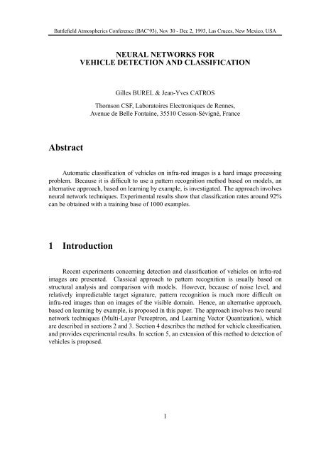
Battleeld Atmospherics Conference (BAC’93), Nov 30 - Dec 2, 1993, Las Cruces, New Mexico, USA
NEURAL NETWORKS FOR
VEHICLE DETECTION AND CLASSIFICATION
Gilles BUREL & Jean-Yves CATROS
Thomson CSF, Laboratoires Electroniques de Rennes,
Avenue de Belle Fontaine, 35510 Cesson-Sévigné, France
Abstract
Automatic classication of vehicles on infra-red images is a hard image processing
problem. Because it is difcult to use a pattern recognition method based on models, an
alternative approach, based on learning by example, is investigated. The approach involves
neural network techniques. Experimental results show that classication rates around 92%
can be obtained with a training base of 1000 examples.
1 Introduction
Recent experiments concerning detection and classication of vehicles on infra-red
images are presented. Classical approach to pattern recognition is usually based on
structural analysis and comparison with models. However, because of noise level, and
relatively impredictable target signature, pattern recognition is much more difcult on
infra-red images than on images of the visible domain. Hence, an alternative approach,
based on learning by example, is proposed in this paper. The approach involves two neural
network techniques (Multi-Layer Perceptron, and Learning Vector Quantization), which
are described in sections 2 and 3. Section 4 describes the method for vehicle classication,
and provides experimental results. In section 5, an extension of this method to detection of
vehicles is proposed.
1

Battleeld Atmospherics Conference (BAC’93), Nov 30 - Dec 2, 1993, Las Cruces, New Mexico, USA
2 The Multi-Layer Perceptron
The Multi-Layer Perceptron is a popular neural network model, which has been
succesfully used in a variety of image processing and pattern recognition applications. The
Multi-Layer Perceptron is trained by the backpropagation algorithm [3]. An example of
such a neural network structure is shown on gure 1. The neuron model is shown on gure
2. It is a weighted summator followed by a non-linear function. First, the neuron’s potential
X j is computed as weighted sum of its inputs O i : X j i W ijO i . Then, the neuron’s
output O j is computed as a non-linear function of its potential: O j FX j tanhX j .
Adding special neurons, called “threshold neurons”, whose output is always 1, improves
the performances of the network.
output vector
input vector
neuron
threshold neuron
input unit
Figure 1: An example of Multi-Layer Perceptron
For instance, for a 3 classes problem, there are 3 neurons on the output layer (one for
each class), and the desired output values are:
1 1 1 for class 1
1 1 1 for class 2
1 1 1 for class 3
2

Battleeld Atmospherics Conference (BAC’93), Nov 30 - Dec 2, 1993, Las Cruces, New Mexico, USA
O
i
W
ij
X
j
F
O
j
Figure 2: The neuron model
Let us note E the mathematical expectancy. The learning algorithm adjusts the
weights in order to provide correct outputs when examples extracted (in a random order)
from a training set are presented on the network input layer. To perform this task, a mean
square error is dened as:
where
e S
output neurons
e MS Ee S
1
obtained output desired output2
2
Let us note g ij e S
, S j the desired outputs, and O j the obtained outputs. It has been
W ij
proved [3]
that g ij j O i ,where
j O j S j F X j when j is on the output layer,
and j
k W jk F X j when j is on another layer. Since the examples are
successors j
extracted in random order (and provided that the training set is signicant), the gradient of
e MS can be approximated by low pass ltering of g ij :
g ij t 1 g ij t g ij t 1
The backpropagation algorithm performs a gradient descent according to:
W ij t g ij t
Once learning is achieved, the network can deal with new data.
the neuron whose output value is the highest determines the class.
For classication,
Acondence measure (between 0 and 1) can also be dened as :
condence = 1 2
( highest output - second highest output )
3

Battleeld Atmospherics Conference (BAC’93), Nov 30 - Dec 2, 1993, Las Cruces, New Mexico, USA
3 Learning Vector Quantization
Learning Vector Quantization is a neural network algorithm proposed by Kohonen
[2], which involves 2 main steps:
Unsupervised representation of the data, using the Topological Maps model.
Supervised ne tuning of the neural network.
3.1 The Topological Maps
The Kohonen network, also known as the “topologic maps model”, is inspired from
a special structure found in some cortex areas (g 3). The neurons are organized in
layers, and, inside a layer, each neuron sends excitatory connections towards its nearest
neighbours, and inhibitory connections towards the other neurons. All neurons receive the
same inputs from the external world.
outputs
Figure 3: The topologic maps model (1D)
inputs
Kohonen simulated the behaviour of this kind of neural network [1], and showed
that it can be approximated by the following algorithm. Let us consider a network with
M neurons, and let us note K the number of inputs, and x [x 1 x 2 x K ] T an input
4

Battleeld Atmospherics Conference (BAC’93), Nov 30 - Dec 2, 1993, Las Cruces, New Mexico, USA
vector. The input vectors are extracted from a set A, called “the learning set”. This
set contains cardA vectors. Each neuron is characterized by a vector of weights
W j [W 1 j W Kj ] T ,where j is the index of the neuron. In response to an input vector x,
the neuron such that the quadratic distance W j x 2 is minimal is called the winner. We
will note O j the output of neuron j:
O j W j x 2
K
W ij x i 2
i1
The learning algorithm is the following (t is the iteration index, and T is the total
number of iterations):
1. t 0
Initialization of the weight vectors W 1 W 2 W M
2. n 1
Let be a random permutation of the set 1 2 cardA
3. Presentation of the vector xn on input.
4. Computation of neurons outputs O j
5. Determination of the winner (neuron k which provides the lowest output)
6. Modication of the weights according to:
7. n n 1
If n cardA,goto(3)
8. t=t+1
If t T go to (2)
W j jk t[x W j ]
The coefcients jk t are of the form t d j k. The distance d denes the dimension
of the network. For 1D networks arranged in ring, such as the one we used for our
application, we have d j k min j k M j k.Weproposetouse:
jk t 0 e d2 jk
2t
2
The constant 0 is called “the learning rate”. Kohonen suggests values around 10 1 .The
standard deviation t decreases with t according to an exponential rule:
t
T 1
T 1
t 0
0
5

Battleeld Atmospherics Conference (BAC’93), Nov 30 - Dec 2, 1993, Las Cruces, New Mexico, USA
It is clear that, at each step, the winner and its neighbours will move their weights
in direction of the input vector x. Hence, the network’s dynamics could be seen as the
result of an external force (adaptation to input vectors), and an internal force (the neighbourhood
relations, that force nearby neurons to have close weights). Kohonen validated
his algorithm on speech data, and showed that the neurons organize their weights in order
to become representative of phonemes. Furthermore, topological relations are preserved
(close neurons react to close phonemes).
y
Figure 4: Self-organization inside a triangle
Properties of Kohonen’s algorithm may be illustrated on a simple example. Let us
assume that the input vectors are of dimension 2, and that their components are coordinates
of a point randomly selected inside a triangle. Each neuron has two weights, so we can
represent it by a point in the 2D plane. Figure 4 shows the network state after learning.
Hence, the neural network, that can be seen as a one dimensional curve, has performed an
approximation of a 2D domain (the triangle).
Kohonen’s algorithm may be easily generalized to higher network’s dimensions. For
example, a 2D network is shown on gure 5.
x
6

Battleeld Atmospherics Conference (BAC’93), Nov 30 - Dec 2, 1993, Las Cruces, New Mexico, USA
neuron
neighbourhood
inputs
Figure 5: Topologic maps model (2D)
3.2 Supervised ne tuning of the neural network
Starting from a topological map which has converged, a class is assigned to each
neuron by majority voting (among the examples for which this neuron is the winner).
Then, the network is tuned in order to improve its classication accuracy. Kohonen has
proposed 3 methods (LVQ1, LVQ2, LVQ3) for ne tuning. LVQ2 is supposed to be an
improved version of LVQ1, and LVQ3 an improved version of LVQ2, although, for some
applications, LVQ1 may provide the best results.
3.2.1 LVQ1
The examples are presented randomly and, for each example, the weights of the
winner ( j)aretunedasbelow(c is the class of the example):
W j x W j
W j x W j
if c j
if c j
7

Battleeld Atmospherics Conference (BAC’93), Nov 30 - Dec 2, 1993, Las Cruces, New Mexico, USA
3.2.2 LVQ2
Let us note j the winner, and k the next-to-nearest neuron. Let us note also
d j x W j and d k x W k . If the class assigned to k is the same as the class of
x, and is different to the class assigned to j, andifd k sd j (s 12), then:
W j x W j
W k x W k
3.2.3 LVQ3
If the class assigned to k is the same as the class of x, and is different to the class
assigned to j, andifd k sd j (s 12), then:
W j x W j
W k x W k
If x, j, k, belong to the same class, then:
W j x W j
W k x W k
4 Classication
Classication of vehicles on infra-red images leads to serious difculties, due to the
following variabilities:
The background is unknown.
The meteorological conditions are uncontrolled.
The orientation of the vehicle with respect to the camera is unknown.
8

Battleeld Atmospherics Conference (BAC’93), Nov 30 - Dec 2, 1993, Las Cruces, New Mexico, USA
The including frame provided by a detector is approximate, hence there may be slight
variations of the apparent size of the vehicle.
These variabilities are taken into account by creating a large training base, containing
various vehicles in many orientations, with many backgrounds and environmental conditions.
Furthermore, to take into account the fact that the including frame is approximate,
slight homotheties are performed on the examples of this data base.
The image to classify is normalized in mean and variance, in order to obtain some
insensibility with respect to camera gain. Then it is normalized in size, because the input
size of a neural network is xed. For our experiments, this size was 24x16pixels.
Six classes of vehicles have been dened: helicopter, truck, and four classes of tanks.
A data base of 945 images of vehicles has been created to train the neural network. A
second data base of 1407 images of vehicles has been created to test the generalization
capabilities of the neural network (these images are not used for training).
Two kinds of neural networks have been compared:
A 3-layer perceptron (384 + 15 + 6 neurons), trained by the backpropagation algorithm
A LVQ network (384 inputs, 32 neurons). The LVQ1 method for ne tuning has been
used.
The obtained generalization rate is:
92% with the 3-layer perceptron
89% with the LVQ network
The required training time (on a Sun workstation) is 10 hours for the 3-layer
perceptron and 30mn for the LVQ network. Classication of a normalized image requires
385x15+16x6 = 5871 multiplications with the 3-layer perceptron, and 384x32 = 12288
multiplications with the LVQ network.
The conclusion is that the performances of these neural networks are quite similar
(92% and 89%), but the MLP is twice faster at recognition. However, since the training
time required by the LVQ network is 20 times lower than the training time required by the
MLP, the LVQ network should be used preferently if one wants to compare quickly the
interest of new training bases.
9

Battleeld Atmospherics Conference (BAC’93), Nov 30 - Dec 2, 1993, Las Cruces, New Mexico, USA
Figure 6 shows the weights of the LVQ network after training. Although the weights
are difcult to interpret, one may recognize patterns similar to helicopters, trucks, and
tanks by careful examination of this image.
Figure 6: Weights of the LVQ network
5 Detection
The approach may be extended to vehicle detection by considering that detection is
some kind of classication problem, where the classes are “vehicle” and “background”.
However, a specic difculty must be stressed: we do not know the distance between the
vehicle and the camera. Hence, the apparent size of the vehicle on the image is unknown.
The proposed approach consists in scanning the image at various resolutions. For
each location and size of the scanning window, the window content is normalized in mean
and variance, then normalized in size, and nally propagated through a neural network.
10

Battleeld Atmospherics Conference (BAC’93), Nov 30 - Dec 2, 1993, Las Cruces, New Mexico, USA
The neural network provides a class (vehicle or background), and a condence associated
to this decision.
All the local decisions are then fused to suppress multiple detections at close spatial
locations. To achieve this task, we search for the strongly overlapping detections. Two
detections are considered as strongly overlapping if the center of one window is included
in the other window. For such congurations, we suppress the detection which has the
lower condence.
For experimentation, we have created a training base of 4647 images (1407 images
of vehicles and 3240 images of backgrounds). It is good to have more backgrounds than
vehicles in the training base, in order to keep the false alarm rate at a low level. MLP
and LVQ networks provide comparable results. On a typical test sequence showing 3
tanks moving at various distances, the 3 vehicles are detected almost on each image of the
sequence, while two or three false alarms may appear stealthy. Since the location of these
false alarms seem to be almost random, they might be suppressed by temporal analysis.
6 Conclusion
An approach to vehicle detection and classication on infra-red images has been
proposed in this paper. The approach is based on learning by example and neural network
techniques. Concerning classication, 6 classes have been dened: helicopter, truck,
and 4 classes of tanks. A neural network has been trained to recognize these classes
independently of vehicle orientation and environment conditions. Two kinds of neural
networks have been compared: the multi-layer perceptron and Kohonen’s learning vector
quantization. Experimental results obtained on 1400 examples show that a classication
rate of 92% can be expected. An extension of this approach for detection purpose has been
proposed. The image is analysed by multi-resolution scanning. For each resolution and
each window location, the content of the window is normalized in size, average brightness,
and contrast. Then, it is propagated through a neural network, which provides a decision
(“vehicle” or “background”) and a condence measure. All the decisions are then fused
across the various resolutions in order to suppress multiple detections at the same location.
The fusion is based on analysis of condence.
References
[1] T. Kohonen, “Self-Organization and Associative Memory”, Springer-Verlag, 1984
11

Battleeld Atmospherics Conference (BAC’93), Nov 30 - Dec 2, 1993, Las Cruces, New Mexico, USA
[2] T. Kohonen, “The Self-Organizing Map”, Proc. of IEEE, vol 78, n o 9, pp 1465-1481,
September 1990
[3] D.E. Rumelhart, G.E. Hinton, R.J. Williams, “Learning internal representations by error
backpropagation”, In Parallel Distributed Processing, D.E. Rumelhart and J.L. Mc
Clelland, Chap 8, Bradford Book - MIT Press - 1986
12