FAST TRIGONOMETRIC FUNCTIONS USING INTEL'S SSE2 ...

FAST TRIGONOMETRIC FUNCTIONS USING INTEL’S SSE2
INSTRUCTIONS
LARS NYLAND AND MARK SNYDER
ABSTRACT. The goal of this work was to answer one simple question: given that the
trigonometric functions take hundreds of clock cycles to execute on a Pentium IV, can they
be computed faster, especially given that all Intel processors now have fast floating-point
hardware The streaming SIMD extensions (SSE/SSE2) in every Pentium III and IV provide
both scalar and vector modes of computation, so it has been our goal to use the vector
hardware to compute the cosine and other trigonometric functions. The cosine function
was chosen, as it has significant use in our research as well as in image construction with
the discrete cosine transform.
1. INTRODUCTION
There are many historical examples where complex instructions can be run faster using
simpler instruction sequences. In Patterson and Hennessey’s Computer Organization and
Design [1], the example of the string copy mechanism in the Intel IA-32 instruction set is
flogged, showing that by using a few efficient instructions, the performance can be drastically
increased. Presumably, the complex instructions were added to the instruction set
architecture to make the job of writing assembly language easier (either by a human or for
a compiler).
Our goal is to explore alternate, accurate implementations of the cosine instruction,
since it meets all of the following criteria:
• the cosine is a heavily used function in many applications.
• the time to execute a cosine instruction on the Pentium IV is lengthy (latency
= 190 - 240 clock cycles with a throughput (restart rate) of 130 cycles [6, 7]).
The Pentium architecture manuals further qualify this, saying that it may vary
substantially from these numbers.
• there are several known methods of accurately computing cosine.
• modern processors (Pentium IV and PowerPC) have vector units as standard equipment.
Searching for methods of cosine to further investigate, we decided to explore the following
three methods—the Taylor Series Expansion for cosine, the Cordic Expansion series,
and Euler’s Infinite Product of sine. We compared them to each other as well as to the
hardware’s current calculation results. Special attention was placed on convergence rates,
as well as the vectorizability of the implementations. The simplest implementations compute
the value of the cosine using C (which relies upon the x87 Floating-point hardware),
but more complex versions using the vector hardware could compute multiple cosine functions
at once (vectorized execution), and the most aggressive implementation would be
to vectorize a single cosine evaluation using the vector hardware. Each of these will be
mentioned in the section on implementation.
1

2 LARS NYLAND AND MARK SNYDER
1.1. Selecting Methods of Calculation. The methods we chose to investigate are all series,
either adding on terms that gradually approach zero, or multiplying terms that gravitate
towards a value of one. Initially, we implemented them in a higher-level language,
tracking the number of terms needed for each version to be accurate within one unit in the
last place. Also considered was the cost of adding each term in to the result. We assume
for all of these that x has the range −π/2 < x < π/2, as all other values of cos(x) can be
determined from this range.
1.2. The Cordic Expansion of Cosine. The CORDIC calculations involve rotation of an
arbitrary vector by known angles, in either a positive or negative direction [2]. The angles
are initially large, and are reduced in half with each iteration. A typical set of rotation
angles is a multiple of the series {1, 1/2, 1/4, 1/8, 1/16, . . . }. The angle of rotation is
specified, and then a running tally of the arctangent of the rotation angles is kept.
To compute a cosine (or sine), a unit vector along the x-axis is rotated by the known
angles in either a positive or negative direction with smaller and smaller steps until the desired
accuracy is achieved. For example, to compute cos(π/3) and sin(π/3), the following
iterative calculation is performed:
[cos(π/3), sin(π/3)] = f(f(f(f(f([1, 0], −π/4), π/8), −π/16), π/32), −π/64)
where f is a rotation of a vector by a specified angle. The choice of whether the rotation
is positive or negative is determined from a running sum of angles. When the sum exceeds
the desired angle, the rotation reverses until the sum is once again less than the desired
angle. This is in contrast to the normal sort of binary choice process that either includes or
ignores a contribution.
We can perform this algorithm through a simple for-loop, with initial conditions z 0 = x,
x 0 = 1, y 0 = 0, and tables of constants for 2 −i values and for tan −1 2 −i values (arrays
t1 and t2, respectively):
for(i = 0; i < numbits; i++)
{
d = (z

FAST TRIGONOMETRIC FUNCTIONS USING INTEL’S SSE2 INSTRUCTIONS 3
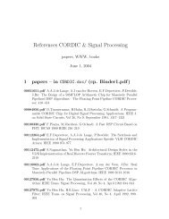
multiple of π (including zero), that the terms approach the value one. This is shown in
figure 1 where the number of terms required is small where cos(x) = 0.
Euler’s infinite product is an interesting formulation, as it is a product rather than a sum,
and the terms approach 1. This means that the bulk of the information is in the first few
terms. We’ll see how this affects the accuracy of a truncated form (finite expansion) in the
section on convergence.
1.4. The Taylor Series Expansion for Cosine. Finally, the most widely known expansion
of the cosine function is the Taylor Series Expansion (technically, the Maclaurin series),
which is:
cos(x) = 1 − x2
2! + x4
4! − x6
6! + x8
8! − . . .
If x < 1, it is obvious that the terms in the sequence rapidly decrease. Indeed, even
when x > 1, there is a point where x n < n!, and from that point on, the terms in the series
rapidly diminish. Given that the domain of interest for x is −π/2 < x < π/2, the only
term that can ever be larger than 1 is x 2 /2, which can be as large as π 2 /4 (approx. 2.5).
After that, the terms rapidly diminish in value.
2. CONVERGENCE AND ACCURACY
2.1. Cost of Calculation and Convergence. There are two main aspects of the cost of
calculating cos(x). The first is the number of terms required to achieve the desired accuracy,
and the second is the cost of calculating each term. In this section, we examine
both for each expansion introduced above. One example where the cost per term is high
is Ramanujan’s method for calculating π [4]. The benefit is that the number of digits is
doubled for each term, so just about any constant cost will outperform most other methods
for finding π.
The first step in choosing an expansion of cosine to implement is to see how many terms
are required to obtain a desired accuracy. The next section examines how much work is
required per term; knowing both the convergence and work per term, we can finally choose
an expansion for implementation.
Our accuracy goal is to match IEEE 754 single and double precision floating-point
numbers. These have 24 and 53 bits in the significand, which represent roughly 7 and 16
decimal digits of precision (we strive to reduce error to be less than within 10 −7 or 10 −16 ,
respectively).
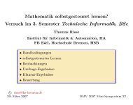
Figure 2 shows the convergence properties for each of the expansions for a variety of
angles. The Taylor Series expansion has much higher accuracy than the other two, and in
fact, it takes a significant number of terms to achieve even the slightest bit of accuracy for
Euler’s Infinite Product.
2.2. CORDIC. The CORDIC method gains one bit of precision per iteration of the loop;
so that means either twenty-four or fifty-three iterations. Unrolling the loop into pairs of
iterations, the last three lines could be removed, and thus requiring five multiplications
and three add/subtracts per bit calculation. Since we see in figure 1 that Taylor requires
significantly fewer terms and note that it is less costly per term, CORDIC is not going to
be as efficient as the Taylor series expansion.
2.3. Euler’s Method. Euler’s method, although an accurate series, converges painfully
slowly—note in figure 1 how many hundreds of terms are required to gain even merely
three digits of precision. Infinite products seem unsuited for approximations.

4 LARS NYLAND AND MARK SNYDER
Number of terms
14
12
10
8
6
4
2
Taylor Series
−90 −45 0 45 90
Angle
Cordic Approximation
60
50
40
30
20
10
−90 −45 0 45 90
Angle
Euler’s Infinite Expansion
400
300
200
100
−90 −45 0 45 90
Angle
FIGURE 1. These graphs show how many terms are required to obtain
accuracy comparable to IEEE 754 Floating-Point (single and double
precision for computing cos(x)). The Taylor series requires more terms
as x moves away from 0, while the Cordic expansion is not dependent
on the value of x, and appears to achieve precision with the number of
terms that match the number of bits in IEEE single and double precision
floating-point numbers (24 and 53 bits). Euler’s infinite expansion
is far worse. The two traces in the rightmost graph are for 2 and 3-digit
precision, as the convergence rate of Euler’s infinite product is nearly
zero.
Error
10 5 Taylor Series
10 0
10 −5
10 −10
10 −15
10 −20
0 5 10 15 20
10 5 Cordic Series
10 0
10 −5
10 −10
10 −15
10 −20
0 20 40 60
Euler’s Infinite Series
5
10
10 0
10 −5
10 −10
10 −15
10 −20
0 20 40 60
FIGURE 2. Convergence. A graph demonstrating the convergence of
different series as terms are added. Each graph shows the reduction in
error as the number of terms is increased. Different values of x are used
to demonstrate the dependence of convergence on the input value. The
values chosen here are 0, 15, 30, 45, 60, 75, and 90 degrees. The Taylor
series converges rapidly, yielding multiple digits per term. The Cordic
series yields one bit per term. Euler’s infinite series converges surprisingly
slowly.
2.4. Taylor Series. As each term is increased (e.g., from x 6 /6!, say, to x 8 /8!), each additional
x must be divided by each additional factor (e.g., 8!/6! = 7 ∗ 8) in the factorial
expansion, and multiplied by the calculated x 2 value. Yet accuracy is completely lost if x n
and n! are computed prior to division. To avoid redundant calculations, the equation can
be even more organized, as follows:
( ( ( ( ( )))))
1 1 1 1 1
cos(x) = 1 − x 2 ·
2! − x2 ·
4! − x2 ·
6! − x2 ·
8! − x2 ·
10!

FAST TRIGONOMETRIC FUNCTIONS USING INTEL’S SSE2 INSTRUCTIONS 5
This form is commonly called Horner’s Rule [5]. Storing these inverse factorial constants
to a table t1 (including the terms’ signs, too), we reduce the problem to the following:
t = [1/(2!), 1/(4!), 1/(6!), 1/(8!), 1/(10!)];
cosx = 1 − x 2 · (t
0 − x 2 · (t
1 − x 2 · (t
2 − x 2 · (t
3 − x 2 · (t 4 ) ))))
3. METHODOLOGY/IMPLEMENTATION
Note: The UNIX program ’Better Calculator’ (’bc’) was used to check accuracy, since
it offers an arbitrary number of digits of precision.
3.1. Taylor Series, In C. This version requires only one multiplication and one addition
per term. While this is very attractive, due to the nesting of calculations, we cannot use
the vector hardware to compute multiple terms at once, since every single instruction is
dependent on the previous. What could be done in the aggressive approach of calculating
one value by vector math
Vectorized calculation of four single-precision terms at once has quite a bit of overhead.
We take one x value and then calculate x 2 , x 4 , x 6 , and x 8 , then pack them into one register
as a = [1|x 2 |x 4 |x 6 ], and another register as b = [x 8 |x 8 |x 8 |x 8 ]—then we can create the
next four terms’ x-dependent portions with a = a · b = ([1|x 2 |x 4 |x 6 ] · [x 8 |x 8 |x 8 |x 8 ] =
[x 8 |x 10 |x 12 |x 14 ]). These registers are packed with a few calls to the shufps instruction,
which is as fast as multiplication (it shifts portions of 128-bit registers around). Storing the
packed constants is handy, at least—we simply have the 32-bit constants stored contiguously
in memory, and load 128 bits at a time. Yet, building up our packed registers leads
to much overhead, and only saves three multiplications and three add/subtracts: the number
of terms necessary determines whether this is more efficient— as we see in figure 1,
only seven terms are required for single-precision, meaning only two batches of four terms
are needed—and indeed, the overhead completely overwhelms the advantage of vectorized
calculation of one series’ terms. Had we required, say, hundreds of terms, each batch afterwards
would require an add, a load, and two multiplies (versus four loads, four adds,
and four multiplies for four terms in the scalar implementation). In short, a nested version
leads to less overhead calculation, and is more efficient.
3.1.1. An Initial Experiment. We took the factorized version of the Taylor series and implemented
it in C. The routine is shown in figure 3, and demonstrates the calculations
required to bring the value of the angle, x, into the range of −π/2 < x < π/2. The coding
style shows a method of essentially avoiding an if-else statement using array indexing. The
original if-else code was similar to:
x = x % pi;
x = abs(x);
if (x > pi/2)
x = pi - x;
else
x = 0 - x;
...
Instead, we always perform the subtraction, using one bit of the quadrant number as an
index to an array that contains [0, π]. For the case when x < π/2, we execute x = 0 − x =
−x. This is fine, as cos(−x) = cos(x). Now we have the angle (less than π/2) whose

6 LARS NYLAND AND MARK SNYDER
extern double ifact[]; // an array with 1/n!, 0 >1)&1] - x; //explained in detail below ()
x2 = - (x*x);
r = ifact[i] * x2;
}
for (i -= 2; i > 0; i-=2){
r += ifact[i];
r *= x2;
}
r += 1;
return r;
FIGURE 3. A C version of the factorization of the Taylor series that
yields one add and multiply per term in the series. Prior to the for-loop,
the code is bringing the value of x into the range −π/2 < x < π/2.
Additionally, we need to determine if cos(x) will be negative. This is
done by computing the quadrant number, in the conventional sense, and
then realizing that quadrants 2 and 3 share a 1-bit in the second bit. We
use that bit as an index to perform the subtraction of x = π − x if x
is in quadrants 2 or 3, and x = 0 − x when x is in quadrants 1 or 4.
The subtraction is always performed, eliminating the need for a branch,
allowing the code to be pipelined in a straightforward manner. This loop
could be unrolled or put in a switch statement, eliminating the loop overhead
and further improving performance. Since the integer ‘quadrant’
initially equals either 0, 1, 2, or 3, and is incremented by one to 1, 2, 3,
or 4, we can shift the binary representations [0001, 0010, 0011, 0100] to
the right by one bit to [0000, 0001, 0001, 0010], then AND them with a
one to get [0000, 0001, 0001, 0000]; thus, we have obtained a ‘zero’ for
the first and fourth quadrants, and a ‘one’ for the second and third quadrants.
magnitude will match the requested angle. This gives us is a fully pipelinable execution
stream, as no branches are executed.
Another discovery in this implementation is the accuracy with which the inverse factorials
can be stored. One feature of floating-point numbers is that the density increases

FAST TRIGONOMETRIC FUNCTIONS USING INTEL’S SSE2 INSTRUCTIONS 7
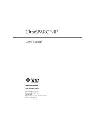
Quadrant image
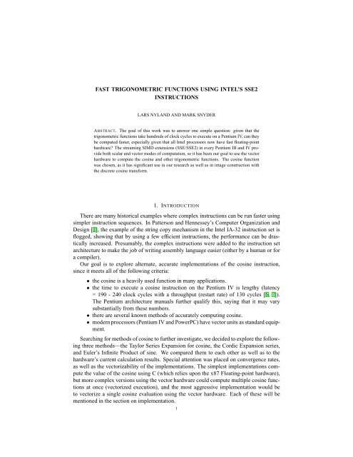
FIGURE 4. We take note of the bottom two bits of the integer acquired
between conversions; this two-bit number, being one of {00, 01, 10, 11},
represents the 1st, 2nd, 3rd, and 4th quadrants. We can AND with 0x1
to get {00, 01, 00, 01}, obtaining ‘0’ when in quadrants one and three
and ‘1’ when in quadrants two and four. In the figure above, notice
that the angles 30, 150, 210, and 330 degrees have identical magnitudes,
yet in quadrants two and four, we would need the value [quadrantSize
- portionInTheQuadrant] instead of simply [portionInTheQuadrant]. If
we convert this number back to a floating-point number, we can multiply
it by π/2, getting either zero or π/2—call this value xpartial.
dramatically as the values approach zero (to a point), so the inverse factorials are accurately
stored. The factorial values, however, would not be accurately stored once they
grow beyond a particular size.
3.1.2. Performance in C. The performance of our C version is notably better than the
hardware version of cosine. On a Pentium IV, a loop of ten million iterations adding up
cosine values took 0.998 seconds with our version and 1.462 seconds using the hardware
instruction. The summation required 0.242 seconds, so the performance comparison is
ours 1.462 − 0.242
=
theirs 0.998 − 0.242 = 1.614
So simply writing cosine as a series calculation, stopping at the full accuracy of double
precision numbers, we can outperform the hardware by over 60%. Recall that this implementation
uses the IA-32 instruction set, so all floating-point calculations are performed
using the x87 floating-point hardware, not the SSE2 hardware.
3.2. ASM Implementation with SSE2 Instructions.
3.2.1. Sign Bits. The first action is masking off the sign bit because we want truncation
to lessen the magnitude always; cos(x) = cos(−x), so this is safe. In order to discern
to which quadrant the input value belongs, we first calculate x 0 · 2/π (pseudo-modulardivision—2/π
is a stored constant). Then, we truncate by converting that to an integer,
reconverting back to floating-point. We decide whether to subtract that truncated value
from π/2 or zero as described with the figure 4. We subtract, getting x partial −(x 0·2/π) =
x ready . Now we have the correct magnitude for cosine calculations. Since the first thing we
do with this adjusted x-value is square it, it doesn’t even matter that cos(−x) = cos(x)—
thinking more generally, this is acceptable for other functions like sine (though we’d add
1 to the integer before the AND instruction, to get a 1 when in the 2nd and 3rd quadrants
instead).
3.2.2. Determining the Quadrant of x. In addition, we need to adjust the sign of the result
at the end. Since we collapsed the four quadrants into one range, we take the integer
from between conversions again from our example, and create either a negative or positive
zero—by adding 1, shifting right one bit, shifting left 31 bits 1 . This will be negative only
for the second and third quadrants, which need a change in sign. Then the result can be
1 To understand what the modifications did, remember that it was an integer of the number of quadrants;
disregarding the upper 30 bits for now, note that the bottom two signify in which quadrant our initial x value
is (adding ‘1’ changes them from [00,01,10,11] to [01,10,11,100]). Shifting those binary numbers right one bit

8 LARS NYLAND AND MARK SNYDER
XOR’d with our calculated magnitude, and if the initial x value was in the second or third
quadrant, this XOR operation will change only the sign bit, leaving the entire rest of the
number alone.
3.2.3. All that is left to do is make the x 2 value and work through the terms. We load
the smallest term’s constant and then repeatedly multiply-by-x 2 and add-the-next-constant,
XORing the sign adjustment after all terms’ calculations.
3.2.4. Double Precision. Making a version for double-precision cosine calculation is nearly
identical; the only two changes are: (a) we must have more terms, and (b) when we mask
the sign, we have to load only the top 32 bits, AND them with the mask, and return them
so that we can then load the entire 64 bits together.
As was mentioned before, an aggressive approach of calculating multiple terms with
the vector-hardware is unsuited; even for doubles, we don’t require nearly enough terms
for the vectorization to even match computation time. However, this is a separate problem
from vectorization for calculating two or four cosines at once, which is quite applicable.
3.3. Vectorized cosine. For more mathematically oriented programs, it is not at all uncommon
to have large sets of data requiring computations on an entire set. A version of
cosine has been made that takes an input array, an output array, and an integer (indicating
the number of cosines to be performed) as parameters. One constraint that had to be overcome
was that although we may load 128 bits from memory not on a 16-byte boundary,
we may not store it off of 16-byte boundaries. So the single-precision function does the
following:
(1) check that a positive number of calculations is requested
(2) compute individual cosines until the address lines up to a 16-byte boundary
(3) compute as many groups of four cosines as remain requested
(4) individually compute any remaining cosines.
3.3.1. Step (1) is merely a safeguard against looping endlessly on towards negative infinity,
should meaningless input be received; step (2) is necessary, because on rare occasions
someone might request storage to begin not on a 16-byte boundary, even though compilers
attempt to line arrays up on larger boundaries. Step (3) does the majority of the calculations.
Step (4) cannot just grab 128 bits, calculate away, and then store only the requested
values. This could conceivably attempt to access memory not allocated to the program;
compilers actually try to leave in extra space to align arrays to 16-byte boundaries when
they can, but this safeguard is necessary.
3.3.2. The vectorized version is more efficient in two main ways—obviously, it gets to
calculate four cosines at a time (other than a possible and negligible few at either end).
But also, imagine the difference between calling any one function a multitude of times
versus calling a vectorized version of the same purpose. All the pushing and popping of
parameter values on the stack while leaving and returning from every single call adds up
significantly, and the vectorized version bypasses basically all of those calls. Other benefits
arise with other functions that require identical preparation prior to calculation— the
method of rounding must be specified for some of the packed conversion instructions (we
were using truncation), and it only needs to be done once, meaning even less instructions
[0,1,1,0] changes the bottom bit to a ‘1’ for the second and third quadrant, and a ‘0’ for the first and fourth quadrant.
Then, shifting thirty-one bits to the left (which is why we ignored all the upper bits), we have constructed
the zero with the appropriate sign, since quadrants two and three have negative cosine values [0x80000000 versus
0x00000000].

FAST TRIGONOMETRIC FUNCTIONS USING INTEL’S SSE2 INSTRUCTIONS 9
function hardware (s) per call (ns) new (s) per call (ns) hw / new percentage
cosf 1.2184 107.8390 0.7074 56.7357 1.9007 190%
sinf 0.9601 82.0035 0.5145 37.4456 2.1899 219%
tanf 1.5203 150.5690 1.0194 100.4800 1.4985 149%
cos 2.0213 200.792 2.2998 228.641 0.8782 87%
sin 1.6809 166.765 2.2799 226.656 0.7357 74%
tan 1.9974 198.410 3.0979 308.455 0.6432 64%
vcosf 0.1099 95.3170 0.0434 28.8220 3.3070 330%
vsinf 0.0909 76.3410 0.0146 14.5850 5.2340 523%
vtanf 0.1196 105.0010 0.0918 91.7760 1.1440 114.4%
vcos 0.1594 159.3970 0.0772 77.1600 2.0658 206%
vsin 0.1293 129.3330 0.0396 39.6230 3.2641 326%
vtan 0.1374 137.3690 0.0753 75.2870 1.8246 182%
expf 5.0331 501.974 3.3309 331.759 1.5135 151%
TABLE 1. Comparison of the original C-library versions to our own.
than a packed version of the function (i.e., a function for calculating exactly four values at
once).
3.4. Double Precision Cosine. A double-precision floating-point vectorized cosine function
was also made which differs only in that: (a) groups of two values are calculated in
the vectorized portion of the process, and (b) more terms were necessary.
4. PERFORMANCE RESULTS
We implemented the above versions, also adding sine and tangent (each using Taylor
Series). On a 2.80 GHz Pentium IV processor, ten million calculations were performed
for each non-vectorized example (1,000,000 for the vectorized versions), and calculation
time due to looping was accounted for and removed. Due to the variable length of completion
times, these percentage values actually fluctuate significantly, on the order of about
30%. Individual test cases of the ten millions (for scalar) and millions (for vectorized) of
calculations are given here.
We operate nearly twice as fast as the hardware for scalar single-precision numbers, for
sine and cosine. Tangent is faster by about 50%, though that can dip to as low as only about
20% faster in specific trials. Incidentally, the double-precision versions for cosine, sine,
and tangent were as accurate—yet they were no more efficient than the hardware. Further
tests to find and eliminate the limiting steps of these functions are under way.
All of our vectorized versions were faster. Vectorized tangent has a slight gain for
single-precision (perhaps insignificant over the scalar version) and around an 80% increase
in the double-precision version. Sine and Cosine showed the absolute most improvement
in vectorized form, though—operating 2 and 3.2 times faster than double-precision calculations,
and operating 3.3 and 5.2 times faster than regular single-precision calculations.
We see that this method of calculations is not just another 5% optimization; the significant
increase in efficiency merits serious checks into the feasibility of integration into
already complete programs, as well as into works still un-begun.

10 LARS NYLAND AND MARK SNYDER
5. OTHER APPLICATIONS
This generalized method of taking Taylor Series expansions, discovering how many
terms are necessary, and creating a Horner factorization with stored constants can be extended
to some other functions.
5.1. Sine. Of course sine may be calculated, nearly identically to cosine; with sine, we actually
took enough terms to calculate values up to π instead of π/2, as this further reduced
the overhead and setup. This is because we now have only two halves of the unit circle
to deal with, instead of four quadrants, and we get to simply shift the integer of number
of halves up 31 bits with no modification. A single multiplication could be gained also by
changing all of the terms to include a π 2n /2 2n for the nth term, and removing an earlier
multiplication by π/2.
5.2. Tangent. Tangent is not as obedient. Its Taylor Series contains constants of 1/3, 1/5,
1/7, and so on, instead of some version of inverse factorials. As a result, it converges much
too slowly; however, the simple fact that tan(x)=sin(x)/cos(x) is quite handy. We may
either calculate both sine and cosine and divide, or get craftier. Based on the quadrant in
which we find the value, we can do the following, recalling that sin 2 (x) + cos 2 (x) = 1:
√
• calculate sine, and then cos(x) = 1 − sin 2 (x). Divide.
• calculate cosine, then sin(x) = √ 1 − cos 2 (x). Divide.
We choose which to use based on which provides better accuracy—first and third quadrants,
we’ll calculate cosine; for second and fourth, sine (accuracy changes based on using
a very small value or a close-to-one value in division). Division is not nearly as fast as
multiplication; for single- and double-precision, it takes 23 or 38 clock cycles for scalar
computations, respectively, and 39 or 69 cycles for packed computations, respectively (see
Intel Pentium 4 [6] and Intel Xeon Processor Optimization [7]). Square Root is the same.
Unfortunately, calling divide and square root after calculating the sine or cosine tends to
kill the efficiency. Results that are just as accurate as the hardware have been obtained, but
they are not yet quicker.
5.3. Exponential Function. Even a non-cyclic function such as exponential can be computed
this way. Its Series is:
e x = ∑ x k
k!
k=1
(This is the sum of the absolute value of all the terms in both sine’s and cosine’s series).
The catch for this function is that we will need increasingly more terms to add up to the
escalatingly large values to be returned. Fortunately, we can implement a little trick:
e x/2 · e x/2 = e x/2+x/2 = e x
If we multiply the input by 1/2 n and then square the result n times, we can bypass the
large values. We could compute e x/2 once and square it, or compute e (x/4) and square
it twice, and so on. This comes at a price, though—despite floating-point numbers being
happily denser nearer to zero, we will eventually be losing accuracy by the final squarings;
it turns out that initially multiplying by 1/16 or 1/32 worked best. Since even floatingpoint
can only store a number but so large, this scheme can accommodate large enough
values until infinity would have to be returned anyways. Alternatively, for e x for extremely

FAST TRIGONOMETRIC FUNCTIONS USING INTEL’S SSE2 INSTRUCTIONS 11
negative values, we get values until our number of digits of accuracy are being surpassed
by the smallness of the answer to return, and zero is returned.
5.4. Inverse Trigonometric Functions. Arc-functions are also possible, though they do
not have as convenient Taylor Series—theirs are slow, like tangent’s Taylor Series. Preliminary
study shows satisfactory accuracy for single-precision versions of arccosine and
arcsine, and a search for the most useful method of obtaining arctangent and for versions
returning a double-precision answer are under way.
6. CONCLUSION
We have shown that utilizing Taylor Series can improve the time necessary for computing
basic functions such as sine and cosine; it gives accurate results as well, for some
other functions such as exponential, tangent, arcsine, and arccosine. Vectorized versions
of these functions give highly improved function speed, often more than tripling the speed.
The generalized method described can be implemented in other limited applications, as
well. Creating a library of these functions could offer a very integratable solution to the
implementation.
REFERENCES
[1] David Patterson and John Hennessey. Computer Organization and Design: The Hardware/Software Interface.
Morgan Kaufmann, 2nd edition, 1997.
[2] Ray Andraka. A survey of CORDIC algorithms for FPGAs. In FPGA’98, the proceedings of the ACM/SIGDA
sixth international symposium on Field Programmable Gate Arrays, pages 191–200, 1998.
[3] Thomas J. Osler and Michael Wilhelm. Variations on vietas and wallis’s products for pi. Mathematics and
Computer Education, 35:225–232, 2001.
[4] John Bohr. Ramanujan’s method of approximating pi, 1998.
[5] Donald E. Knuth. The Art of Computer Programming, v.2, Semi-numerical Algorithms. Addison-Wesley, 2nd
edition, 1998.
[6] Intel Corporation. Intel Pentium 4. 2002.
[7] Intel Corporation. Intel Xeon Processor Optimization. 2002.