Subevent analysis for the Tabas earthquake of September 16, 1978 ...

More documents

Recommendations

Info

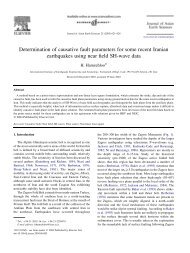
18 I. Sarkar et al. / Physics of the Earth and Planetary Interiors xxx (2005) xxx–xxx Table 2 Estimated source parameters of the different subevents Sub-event Station f c (Hz) M 0 (N m) M w r (km) E (erg) σ (bar) D (m) L (km) S1 Tabas 0.19 0.01 × 10 20 5.97 3.9 2.4 × 10 21 7.4 Boshroyeh 0.01 × 10 20 5.97 2.4 × 10 21 7.4 S2 Boshroyeh 0.10 0.70 × 10 20 7.20 7.5 1.7 × 10 24 75.5 Deyhook 0.90 × 10 20 7.27 2.8 × 10 24 95.3 25.5 18.80 Tabas 1.02 × 10 20 7.30 3.6 × 10 24 108.0 S3 Boshroyeh 0.10 0.12 × 10 20 6.69 7.5 5.0 × 10 22 12.7 Deyhook 0.30 × 10 20 6.95 3.1 × 10 23 31.8 8.49 18.80 Tabas 0.20 × 10 20 6.83 1.4 × 10 23 21.1 S4 Deyhook 0.14 0.04 × 10 20 6.37 5.3 1.5 × 10 22 11.7 2.27 13.29 S5/S6 Deyhook 0.14 0.04 × 10 20 6.37 5.3 1.5 × 10 22 11.7 2.27 13.29 S6/S5 Tabas 0.14 0.04 × 10 20 6.37 5.3 1.5 × 10 22 11.7 to the corresponding observed SH-wave displacement spectra (|U(f)|) in the high fidelity frequency band viz. (0.1–0.2) Hz to (4.0–6.0) Hz (see Fig. 6). In this mathematical expression (5), f denotes the frequency expressed in Hz, t the travel time, GS(R) geometrical spreading, and R the source receiver distance. GS(R)=R −1 for R ≤ R y and GS(R)=(RR y ) −0.5 for R > R y . R y may be taken as twice the thickness of crust (Herrmann and Kijko, 1983). We have taken R y as 90 km (Berbarian, 1982). The term exp(−πft/Q S ) accounts for the attenuation at high frequencies and describes inelastic attenuation of waves (e.g. Dainty, 1981; Fletcher, 1995). The best-fit Brune model spectra (Fig. 6) can now be extrapolated to the long periods to provide the most appropriate estimates for the corner frequency (f c ) and the zero spectral level (Ω 0 ) for each case (Fig. 6). The seismic moment (M 0 ) is then given by M 0 = FΩ 0 where F =4πρβ 3 /F SH R θφ (Hanks and Thatcher, 1972), ρ is the density, β shear wave velocity, F SH is the free surface effect (=2) and R θφ is the radiation pattern calculated from the estimated fault plane solution. The moment magnitude (M w ) can be estimated from M w = (2/3)log M 0 − 10.7, where M 0 is expressed in dyne cm (Lay and Wallace, 1995). The radius of equivalent circular dislocation surface (r) isr = 2.34β/2πf c , the energy radiated in the form of shear waves (E) is E = (128π 3 ρβR 2 Ω0 2 f c 3 )/15 and the apparent stress drop (σ) isσ = µE/M 0 , where µ is rigidity modulus (Hanks and Thatcher, 1972). We use these formulae to estimate the source parameters of the different sub-events (S1, S2, S3, S4, S5 and S6) (see Table 2). We have assumed an average shear wave velocity (β) = 2.0 km/s, rigidity modulus (µ) = 2.0 × 10 11 dynes/cm 2 and average density (ρ) = 1.5 g/cm 3 for our calculations. Although there is no detailed seismic velocity structure available for the Tabas region, Berbarian (1982) and Niazi and Shoja-Taheri (1985) inverted regional and local data to suggest a shear wave velocity of about 2 km/s in the shallow (
I. Sarkar et al. / Physics of the Earth and Planetary Interiors xxx (2005) xxx–xxx 19 the estimated values of R we now surmise (see Fig. 1a) that the locations of S5 and S6 epicenters possibly coincide. The indirect implication of this observation is that perhaps S5 and S6 in actuality represent the same sub-event. 5. Discussion Shoja-Taheri and Anderson (1988) have identified signatures of four sub-events on the strong motion records at Tabas, Deyhook, Boshroyeh and Ferdows (S1, S2, S3 and S4 in their Fig. 4) and have suggested plausible epicentral locations for these subevents (identified as 1–4 in their Fig. 6). The sub-events are seen more distinctly on their horizontal records from Deyhook (see their Fig. 4) and correspond to the phases marked as S2, S3, S4 and S5 on our Deyhook SH-wave accelerograms and velocity seismograms (see our Fig. 1b). Note that the location of the first sub-event S1 of Shoja-Taheri and Anderson (1988) (marked as 1 in their Fig. 6) coincides with the event location of Engdahl et al. (1998). This location is also our assumed location of S2 sub-event observed on our ‘SH-wave’ accelerograms and velocity seismograms, from where presumably the main phase of energy was released. Also our estimated location of the epicenter S3 (see Fig. 1a) is close, less than 10 km to the west of the location of corresponding sub-event 2 epicenter of Shoja-Taheri and Anderson (1988) (marked as 2 in their Fig. 6). Also our suggested locations of S4 and S5/S6 epicenters are slightly west of the locations of 3 and4ofShoja-Taheri and Anderson (1988). Hartzell and Mendoza (1991) inverted simultaneously the strong motion records from Tabas, Deyhook and Boshroyeh and also WWSSN teleseismic records to provide details of the earthquake rupture history. Their numerical calculations could provide three wellresolved sources of energy. Of these, two main source regions of energy release, one around the hypocenter and the other 30 km NW of the hypocenter, extended from the surface to a depth of about 10 km. A third estimated source of energy release is from a region, at about 14 km depth, angled upwards towards Tabas town, approximately 50 km NW of the hypocenter. We may note here that our analysis estimates that (i) S3 hypocentre is located about 25 km NW of the estimated S2 hypocentre, (ii) both S2 and S3 hypocentres lie at a depth of 10 km approximately and (iii) S4 and S5/S6 also possibly lie to the NW of S3. The source time function for the Tabas rupture process has been modeled by various inversion procedures. For example, Hartzell and Mendoza (1991) simultaneously inverted near field and far field P wave data from WWSSN networks to find the best fitting sourcetime function. Assuming a circular rupture and a constant propagating stress drop, they suggested either (i) a simple triangular source-time function with 0.7 s duration or (ii) a modified Kostrov source-time function with 2.9 s duration. They preferred the latter model because this gave an estimated moment and maximum displacement that was more consistent with the longperiod surface waves and field observations. Walker et al. (2003), while ignoring the possibility that several asperities ruptured during the earthquake process, inverted long period P and SH wave data from WWSSN network to suggest a single, simple rupture event lasting for about 18 s. Obviously none of these simplified models are appropriate representation of the details of the complex Tabas rupture process. We have estimated that the S3 phase of energy (corresponding to S2 phase of Shoja-Taheri and Anderson, 1988) was released about 9 s after the release of S2 phase of energy (corresponding to S1 phase of Shoja- Taheri and Anderson, 1988). Also our analysis of the Tabas, Deyhook and Boshroyeh ‘SH-wave; accelerograms seem to suggest the occurrence of a sub event (designated S1 by us), about 5–6 s prior to the main phase of energy release (S2). Shoja-Taheri and Anderson (1988) have suggested, on the basis of an analysis of Deyhook records, that the last distinct phase of energy (designated S4 by them and as S5 by us) was released 22 ± 3 s after the first phase of energy (designated S1 by them and S2 by us) and also estimated that the rupture velocity is about 2.7 ± 2 km/s. The Deyhook transverse acceleration and velocity records (see Fig. 1b) show that the (S5–S2) shear wave arrival time is of the order of 36.4 s. We have suggested from the best-fit Brune ω −2 model spectrum that this sub-event is located about 66 km away from Deyhook, which, for a rupture velocity of 2.7 km/s, implies that S5 phase of energy was released approximately 20 s after the release of S2 phase of energy, a result that is in conformity to Shoja-Taheri and Anderson (1988)’s result. Again, from Deyhook transverse acceleration and velocity records (see Fig. 1b) we find that (S4–S2) shear
Page 1 and 2: Physics of the Earth and Planetary
Page 3 and 4: I. Sarkar et al. / Physics of the E
Page 17: I. Sarkar et al. / Physics of the E

Subevent analysis for the Tabas earthquake of September 16, 1978 ...

Create successful ePaper yourself

Delete template?

Save as template?