30) Review of Asymptotic Theory
30) Review of Asymptotic Theory
30) Review of Asymptotic Theory

You also want an ePaper? Increase the reach of your titles
YUMPU automatically turns print PDFs into web optimized ePapers that Google loves.
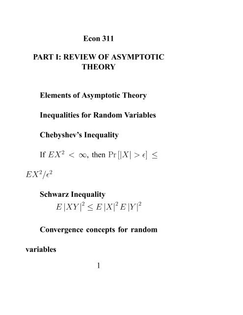
Econ 311<br />
PART I: REVIEW OF ASYMPTOTIC<br />
THEORY<br />
Elements <strong>of</strong> <strong>Asymptotic</strong> <strong>Theory</strong><br />
Inequalities for Random Variables<br />
EX 2 / 2<br />
Chebyshev’s Inequality<br />
If EX 2 < ∞, thenPr [|X| >] ≤<br />
Schwarz Inequality<br />
E |XY | 2 ≤ E |X| 2 E |Y | 2<br />
Convergence concepts for random<br />
variables<br />
1
Almost sure convergence<br />
X T (ω)<br />
as<br />
−→ X(ω) iff<br />
2
Pr [lim T →∞ |X T (ω) − X(ω)| ≤ ] =<br />
1 ∀ >0<br />
Strong Law <strong>of</strong> Large Numbers<br />
Let X T = 1 TX<br />
Y i and X = lim T →∞ E(X T )<br />
T<br />
be finite. If X T (ω)<br />
i=1<br />
as<br />
−→ X, then{Y i } obeys<br />
the SLLN. Sufficient conditions for {Y i } to<br />
obey the SLLN:<br />
{Y i } independent and<br />
(Kolmogorov)<br />
∞X<br />
i=1<br />
1<br />
i 2V (Y i) < ∞<br />
{Y i } iid and E(Y i ) exists (also a necessary<br />
condition)<br />
3
Convergence in rth Moment<br />
X T (ω)<br />
rth moment<br />
−→<br />
X if E(X r T ) and<br />
E(X r ) exist and lim T →∞ E [|X T − X| r ]=0<br />
Convergence in Probability<br />
X T (ω)<br />
p<br />
−→ X(ω) iff<br />
lim T →∞ Pr [|X T (ω) − X(ω)| >]=0<br />
∀ >0<br />
In other words, ∃ T 0 such that<br />
T > T 0 =⇒ Pr [|X T − X| >]=0. If<br />
X T<br />
p<br />
−→ k, a constant, we write plimX T = k.<br />
4
Weak Law <strong>of</strong> Large Numbers<br />
Let X T = 1 TX<br />
Y i and X = lim T →∞ E(X T )<br />
T<br />
i=1<br />
be finite. If X T (ω)<br />
p<br />
−→ X, then{Y i }<br />
obeys the WLLN. A sufficient condition<br />
for {Y i } to obey the WLLN is that<br />
1<br />
TX<br />
lim T −→∞ V (X<br />
T 2<br />
T )=0.<br />
T =1<br />
Slutsky Theorem<br />
X T<br />
p<br />
−→ X and g(X) continuous =⇒<br />
g(X T )<br />
p<br />
−→ g(X).<br />
If X is a constant, we write plim g(X T )=<br />
g(plim X T ). So if g(X T ) is an estimate<br />
5
<strong>of</strong> some parameter and we don’t know the<br />
distribution <strong>of</strong> g(X T ), then approximate it<br />
with the distribution <strong>of</strong> g(X).<br />
Convergence in Distribution<br />
X T<br />
d<br />
−→ X (rv or constant) iff F T → F<br />
pointwise, where F is the cdf <strong>of</strong> X.<br />
Preliminary Results<br />
d<br />
1. g(·) continuous and X T −→ X =⇒<br />
d<br />
g(X T ) −→ g(X)<br />
p<br />
d<br />
d<br />
2. X T −→ Y T and Y T −→ Y =⇒ X T −→<br />
p<br />
Y where X T −→ Y T means<br />
lim<br />
T −→∞ Pr[|X T(ω) − Y T (ω)| >ε]=0.<br />
Man and Wald Theorem<br />
6
d<br />
X T −→ X and Y T<br />
d<br />
1. X T + Y T −→ X + c<br />
p<br />
−→ c =⇒<br />
2. X T Y T<br />
d<br />
−→ Xc<br />
3. The limit <strong>of</strong> the joint distribution <strong>of</strong><br />
(X T ,Y T ) exists and equals the joint<br />
distribution <strong>of</strong> (X, c).<br />
Delta Method<br />
If {α T } is a sequence <strong>of</strong> nonstochastic<br />
numbers tending to ∞, α T (Z T − θ)<br />
d<br />
−→ X<br />
where θ is a constant, and g 00 (·) exists, then<br />
α T [g(Z T ) − g(θ)]<br />
d<br />
−→ g 0 (θ)X. If g 00 (·)<br />
exists and √ T (Z T − θ)<br />
d<br />
−→ N(0,σ 2 θ ),then<br />
√<br />
T [g(ZT ) − g(θ)]<br />
d<br />
−→ N ¡ 0,g 0 (θ) 2 σ 2 θ¢<br />
.<br />
7
Comparing Convergence Concepts<br />
X T<br />
X T<br />
d<br />
−→ X<br />
as<br />
−→ X =⇒ X T<br />
p<br />
−→<br />
⇑ X =⇒<br />
X T<br />
rth moment<br />
−→<br />
X<br />
If X is a constant, then<br />
X T<br />
d<br />
−→ X =⇒ X T<br />
p<br />
−→ X.<br />
8
Central Limit Theorems<br />
Lindberg-Levy CLT<br />
{Y t } iid, Ȳ = 1 T<br />
TX<br />
t=1<br />
E(Y t )=µ, V (Y t )=<br />
Liapounov CLT<br />
Y t<br />
σ 2 =⇒ √ T (Y − µ)<br />
d<br />
−→ N(0,σ 2 ) .<br />
{Y T } independent, E(Y t )=µ t ,V(Y t )=<br />
σ 2 t ,andE(Y 3<br />
t ) exist =⇒ √ T (Y − µ)<br />
d<br />
−→<br />
N(0, σ 2 ),where<br />
σ 2 = lim 1 T<br />
TX<br />
σ 2 t.<br />
t=1<br />
9
[1] Amemiya, Advanced Econometrics,<br />
1985, chapter 3.<br />
[2] Greenberg and Webster, Advanced<br />
Econometrics, 1991, chapter 1.<br />
10
PART II: ANALOGY PRINCIPLE AND<br />
EXTREMUM ESTIMATORS<br />
METHODS OF ESTIMATION<br />
Consider Four Methods<br />
(1) MLE<br />
(2) [Nonlinear] Least Squares<br />
(3) Methods <strong>of</strong> Moments<br />
(4) GMM<br />
11
Modern Methods in Econometrics<br />
These methods are not always distinct in a<br />
particular problem:<br />
e.g.<br />
classical normal linear regression<br />
model<br />
Y t = X t β + U t U t ∼ N(0,σ 2 u)<br />
U t<br />
iid<br />
X t<br />
Fixed constant<br />
P<br />
Xt X 0 t<br />
T<br />
Full rank .<br />
In this case, OLS is all four rolled into one.<br />
12
One basic principle underlies these methods:<br />
Analogy Principle: (Large Sample version).<br />
This is due to Karl Pearson or Goldberger.<br />
Suppose ∃ true model in population<br />
M(Y,X,θ 0 )=0, an implicit equation. θ 0<br />
is a true parameter vector. Defined for other<br />
values <strong>of</strong> θ (at least some other). Construct<br />
some “criterion” or function <strong>of</strong> model and<br />
data:<br />
Q(Y,X,θ)<br />
which has property P in the population when<br />
13
θ = θ 0 .<br />
In the sample, construct something which<br />
converges to Q for each θ<br />
14
Q T (Y,X,θ) almost surely, uniformly<br />
−−−−−−−−−−−−−−−−→ Q<br />
for some θ ∈ Θ<br />
(T isthesamplesize)<br />
and mimics in sample properties <strong>of</strong> Q in<br />
population.<br />
Let ˆθ T be the estimator <strong>of</strong> θ 0 in sample<br />
T formed from the analog in sample<br />
(which causes sample Q T (<br />
) to have the<br />
Property).<br />
Then, we have under “regularity conditions”<br />
∧<br />
θ T p −→<br />
θ 0<br />
15
Regularity conditions:<br />
(Basic ideas)<br />
(a) Identification: only one value <strong>of</strong> θ<br />
satisfies P in population (at least in nbd <strong>of</strong><br />
θ 0 ). One can define this using a Local vs. a<br />
Global definition.<br />
(b) Need Q T ( ∧ θ T ) to converge “nicely”: in<br />
particular<br />
Q T (θ) → Q(θ)<br />
all θ ∈ Θ.<br />
Need convergence to be uniform:<br />
i.e. if ∧ θ T → C, Q T ( ∧ θ T ) → Q(C) .<br />
This is the intuition underlying the method:<br />
Consider the property that<br />
Q is maximized at θ = θ 0<br />
(in population).<br />
16
Select criterion so Q T (θ) → Q<br />
for<br />
all θ ∈ θ<br />
=<br />
.<br />
Select b θ T maximize Q T (θ) for each T .<br />
Then if convergence is “O.K” we get that<br />
under regularity, we have convergence in the<br />
sample to maximizer in the population.<br />
Now suppose θ = {1, 2, 3} a finite set.<br />
..<br />
·<br />
θ ∧ assumes only one <strong>of</strong> 3 values.<br />
by (a) Q is maximized at one <strong>of</strong> these.<br />
each θ.<br />
by hypothesis Q T (θ)<br />
p<br />
−→ Q(θ)<br />
for<br />
17
..<br />
·<br />
the rule picks<br />
∧<br />
θ T<br />
= argmax Q T (θ).<br />
This must work for T “big enough,”<br />
because Q T<br />
p −→<br />
Q for each θ. Why<br />
As T gets “big” we get Q T (θ) arbitrarily<br />
close to Q(θ)<br />
..<br />
·<br />
evaluate Q T (θ) at θ =1, 2, 3<br />
∧<br />
θ is the value that maximizes Q(θ), but<br />
maximizing value is θ 0 .<br />
..<br />
·<br />
∧<br />
θ T p −→<br />
θ.<br />
Otherwise one gets a contradiction Q T ( ∧ θ)<br />
18
Q(θ 0 ). This can’t happen as Q T → Q since<br />
θ 0 is defined to be the maximizing value.<br />
Here Principle P is extremum principle:<br />
Examples<br />
max : Maximum Likelihood<br />
min : Nonlinear Least Squares.<br />
Some Definitions<br />
Convergence <strong>of</strong> sequences <strong>of</strong> Functions:<br />
(Assume Real)<br />
For each x ∈ S form a sequence {F n (x)} .<br />
Let B be the set <strong>of</strong> points for which F n (x)<br />
19
converges.<br />
F (x) = lim<br />
n→∞<br />
F n (x) if x ∈ B. Then we<br />
call F (x) a limit function. {F n (x)} converges<br />
pointwise on B.<br />
Basic Fact:<br />
Pointwise convergence is not enough to<br />
guarantee that if F n has a property (continuity,<br />
differentiability, etc.) that the property is<br />
inherited by F .<br />
For this notion we need uniform convergence.<br />
(Sufficient Condition)<br />
20
e.g. does lim<br />
x→x0<br />
F n (x) =F n (x 0 ) for each n<br />
⇒ lim<br />
x→x0<br />
F (x) =F (x 0 )<br />
(where F is the limit function)<br />
e.g. does lim lim F n (x) = lim lim F n (x)<br />
x→x0 n→∞ n→∞ x→x0<br />
No, not in general.<br />
Example:<br />
F n (x) =n 2 (x)(1 − x) n ; 0 ≤ x ≤ 1<br />
lim n→∞ F n (x) =0<br />
for each fixed x<br />
but set x = 1<br />
µ n +1<br />
1<br />
lim n→∞ F n<br />
n +1<br />
∞<br />
µ µ n 1 n<br />
= n 2 →<br />
n +1 n +1<br />
A sequence <strong>of</strong> functions {F n } converges<br />
21
uniformly to F on B if for every ε>0 , ∃ an<br />
N (depending only on ε and not on x) such<br />
that for all<br />
n>N⇒ |F n (x) − F (x)|
(y, x) related to θ in population.<br />
Q 0 = Q<br />
(Population moments (y, x))<br />
In the sample<br />
∧<br />
θ T = θ (Sample moments)<br />
Now two cases:<br />
Case A: Q T<br />
= Q (OLS) Slutsky’s<br />
Theorem:<br />
ˆθ T = θ (Sample Moments)<br />
Sample moments → population moments<br />
Given (a)<br />
∧<br />
θ T<br />
p<br />
−→ θ 0<br />
(both solve same equation – we don’t need B.)<br />
23
Case B: Q T<br />
p<br />
−→ Q We need uniform<br />
convergence in order for Q T (sample moments)<br />
→ Q<br />
for (sample moments) and<br />
ˆθ → θ for (population moments)<br />
Example:<br />
OLS<br />
Y t = X t β 0 + U t E(U t )=0 Var(U t )=σ 2 u<br />
E(X 0 tU t )=0<br />
E(X 0 tX t )= X xx positive definite E(X0 tY t )= X xy<br />
Assume (Y t X t ) iid sequence.<br />
In population: E(X 0 tU t )=0<br />
24
or<br />
Q :<br />
Xty 0 t = XtX 0 t β 0 + XtU 0 t<br />
X<br />
= X β 0 +0<br />
xy xx<br />
β 0 = X −1 X<br />
xx xy<br />
in sample:<br />
⎛X<br />
∧<br />
β T = ⎝<br />
T<br />
X 0 tX t<br />
⎞<br />
⎠<br />
X<br />
⎝<br />
−1 ⎛<br />
T<br />
X t Y t<br />
⎞<br />
⎠<br />
..<br />
·<br />
rhs →<br />
∧<br />
β → β 0<br />
³X<br />
´−1 X<br />
xx xy<br />
Another Analogy:<br />
Define U as Û<br />
E(X 0 tU t )=0 b U = y − x b β mimics<br />
U !<br />
Pick ∧ β as<br />
25
(1)<br />
1<br />
T<br />
1<br />
T<br />
(Leads to Different Analogy)<br />
then<br />
X ∧<br />
Xt (Y t − X tβ)=0<br />
⎛X<br />
⎞<br />
X X t X t<br />
Xt Y t = ⎝ ⎠ β<br />
∧<br />
ObservethatwehavethatwhenX t =1<br />
T<br />
∧<br />
β =<br />
X<br />
Yt<br />
T<br />
:themean.<br />
Extremum Principle which underlies Nonlinear<br />
Least Squares (and MLE) is also illustrated<br />
in linear regression:<br />
Y t = X t β +[X t (β 0 − β)+U t ]<br />
(Y t − X t β) 2 =(β 0 − β) 0 XtX 0 t (β − β 0 )<br />
26
+2U t X t (β − β 0 )+U 2 t .<br />
Let Q = E[Y t − X t β] 2<br />
= (β −<br />
β 0 ) 0 X xx (β − β 0)+σ 2 u .SinceU t and X t<br />
independently E(U t )=0.<br />
min Q wrt β at min we have β = β 0 .<br />
β = β 0 .<br />
Now in population: min wrt β occurs at<br />
..<br />
·<br />
Form Sample Analog:<br />
Q T = 1 T<br />
TX<br />
(Y t − X t β) 2<br />
t=1<br />
Analog Principle:<br />
27
plim Q T = plim 1 T<br />
TX<br />
(Y t − Xtβ) 0 2<br />
t=1<br />
=(β −β 0 ) 0 X xx (β −β 0)+σ 2 U<br />
pick ∧ β to min . Can’tmakeitanysmallerthan<br />
β 0 in limit. Get contradiction unless ∧ β → β 0 .<br />
28
Extremum Principle:<br />
In the population<br />
Y t = g(X t ; θ)+[g(X t ; θ 0 ) − g(X t ; θ)] + U t<br />
assume (U t ,X t ,Y t ) iid<br />
U t ⊥X t<br />
..<br />
·<br />
U t ⊥g(X t ; θ) all θ<br />
Q = E(Y t −g(X t ; θ)) 2 = E [g(X t ; θ 0 ) − g(X t ; θ)] 2 +σ 2 U<br />
at θ = θ 0 ,Qminimized in population.<br />
If θ = θ 0 is the only such value, model is<br />
29
identified<br />
(wrt Q criterion).<br />
Analogy in Sample: Pick<br />
Q T (θ) = 1 TX<br />
(Y t − g(X t ; θ)) 2<br />
T<br />
t=1<br />
∧<br />
θ T = argmin Q T (θ)<br />
min Q T (θ) for all T : Q T (ˆθ T )
U t ⊥g(X t ; θ 0 ) ⇒ E(U t g(X t ; θ)) = 0<br />
(only one implication <strong>of</strong> ⊥).<br />
Now we may write<br />
Y t − g(X t ; θ) =U t<br />
..<br />
·<br />
E [(Y t − g(X t ; θ)] = 0<br />
just by analogy.<br />
Sample b Q = 1 T<br />
TX<br />
(Y t − g(X t ; θ))g(X t ; θ).<br />
t=1<br />
Find θ which set = ˆQ (or is close to zero<br />
as possible). Now we can make analogy<br />
complete.<br />
Maximum Likelihood:<br />
31
Suppose the joint density <strong>of</strong> data<br />
f(y t ,x t ; θ) =f(y t | x t ; θ)f(x t )<br />
assume that x t is “exogenous” i.e. density <strong>of</strong><br />
x t is uninformative about θ.<br />
Assume random sampling. Then, we<br />
have that<br />
Q<br />
$ = T f(y t ,x t ; θ)<br />
t=1<br />
or taking (y t ,x t ) as data, is a function <strong>of</strong> θ<br />
TX<br />
ln £ = ln f(y t, x t ; θ) =<br />
TX<br />
ln f(x t )<br />
t=1<br />
t=1<br />
TX<br />
ln f(y t | x t ,θ)+<br />
t=1<br />
32
Principle <strong>of</strong> Maximum Likelihood: Pick<br />
θ thatmaximizes£. Thisisanextremum<br />
version <strong>of</strong> analogy principle.<br />
In the population define<br />
33
Q = E θ0 (ln f(y t ,x t ; θ))<br />
Z<br />
= [ln f(y t ,x t ; θ)] f(y t ,x t ; θ 0 )dy t dx t<br />
(Assume exists)<br />
This is always at max when θ = θ 0 .<br />
Why<br />
because<br />
· ¸ f(yt ,x t ; θ)<br />
E θ0<br />
f(y t ,x t ; θ 0 )<br />
=1<br />
=<br />
Z f(yt ,x t ; θ)<br />
f(y t ,x t ; θ 0 ) f(y t,x t ; θ 0 )dy t dx t =1.<br />
Now apply Jensen’s inequality<br />
E(ln(x)) ≤ ln E(x)<br />
(ln is concave function)<br />
· ¸¸<br />
f(yt ,x<br />
..E<br />
·<br />
t ; θ)<br />
θ0<br />
·ln<br />
≤ 0<br />
f(y t ,x t ; θ 0 )<br />
34
..E<br />
·<br />
θ0 [ln f(y t ,x t ,θ)] ≤ E θ0 [ln f(y t ,x t ,θ 0 )] ∀θ<br />
Identified globally in the population if the<br />
inequality is strict for all θ 6= θ 0 .<br />
..<br />
·<br />
Construct sample Q b :<br />
$ = 1 TX<br />
ln f(y t ,x t | θ)<br />
T<br />
t=1<br />
b θ =argmax£ (assume exists)<br />
..<br />
·<br />
if Q T → Q all θ ∈ Θ<br />
and if convergence is uniform, consistency<br />
follows immediately.<br />
Local form <strong>of</strong> the principle<br />
Z<br />
Q(θ) = ln f(y; θ)f(y; θ 0 )dy = E θ0 (ln f(y; θ))<br />
35
Max θ<br />
FOC:<br />
SOC:<br />
Z ¸<br />
·∂ ln f(y, θ)<br />
f(y; θ 0 )dy =0<br />
∂θ<br />
Z ∂ 2 ln f(y; θ)<br />
∂θ∂θ 0 f(y; θ 0 ) negative definite<br />
Requirement:<br />
1<br />
TX<br />
T<br />
t=1<br />
1<br />
TX<br />
T<br />
t=1<br />
∂ 2 ln f<br />
∂θ∂θ 0<br />
(Local conditions)<br />
∂ ln f(y t ; θ)<br />
∂θ<br />
=0<br />
negative definite<br />
Either way, same basic idea. For each T<br />
pick ˆθ T such that:<br />
Q T<br />
³<br />
bθT´<br />
>Q T (θ).<br />
Now if Q T<br />
³<br />
bθT´<br />
→ Q(lim b θ T ) (uniform<br />
36
convergence) we get Q( b θ T ) > Q(θ θ ),<br />
assumed to be a maximum value. Thus we get<br />
a contradiction unless plim b θ T = θ 0 . Q.E.D.<br />
To be more precise: we need definitions.<br />
Random Function: Let (Ω, A,P) be probability<br />
space and let Θ ⊂ R k . A real function<br />
F (θ) =F (θ, w) on Θ× Ω is called a random<br />
function on Θ if for every t ∈ R 1 and θ ∈ Θ<br />
{w ∈ Ω : F (θ, w)
Proposition:<br />
If ϕ(θ, x) is continuous real<br />
function on Θ × R n<br />
where Θ is compact,<br />
sup θ∈Θ ϕ(θ, x) and inf ϕ(θ, x)<br />
θ∈Θ<br />
are continuous functions.<br />
Pro<strong>of</strong>: See any Real Analysis text (see, e.g.<br />
Royden).<br />
Proposition: If for almost all values <strong>of</strong> x in<br />
X, g(x,θ) is continous wrt θ at point θ 0 ,and<br />
if for all θ in nbd <strong>of</strong> θ 0 we have<br />
|g(x, θ)|
Z<br />
lim<br />
θ→θ 0<br />
g(x, θ)dF (x) =<br />
Z<br />
g(x, θ 0 )dF (x)<br />
i.e. lim θ→θ0 E(g(x, θ)) = E(g(x, θ 0 ))<br />
Proposition:<br />
If for almost all values <strong>of</strong> x in<br />
X and for a fixed value <strong>of</strong> θ<br />
(a)<br />
(b)<br />
∂g(x, θ)<br />
exists (in nbd <strong>of</strong> θ)<br />
∂θ<br />
g(x, θ + h) − g(x, θ)<br />
¯ h ¯
function to another. Let F (θ) and F n (θ) be<br />
random functions on Θ ⊂ R k for each θ ∈ Θ.<br />
1<br />
F n (θ) almost surely converges to F (θ) as<br />
n →∞if<br />
P {w | lim n→∞ |F n (θ, w) − F (θ, w)| n 0 (θ, ε) i.e. the set S θ such that<br />
|F n (θ, w) − F (θ, w)| ≥ ε if n ≥ n 0 (θ, ε)<br />
has no probability. Now: S = ∪ S θ may<br />
θ∈θ<br />
=<br />
have non-negligible probability even though<br />
any one set has negligible probability. We<br />
avoid this by the following definition.<br />
40
Definition: Almost sure uniform convergence:<br />
(2) F n (θ) → F (θ) almost surely uniformly in<br />
Θ<br />
if sup |F n (θ) − F (θ)| → 0 almost surely as<br />
θ∈Θ<br />
n →∞<br />
i.e. for every ε>0 and w ∈ Ω.<br />
P {w : lim n→∞ sup θ∈Θ |F n (θ, w) − F (θ, w)| ≤ ε} =<br />
1.<br />
In this case, the negligible set not indexed by<br />
θ.<br />
41
Definition:<br />
Convergence in Probability. Let<br />
F n (θ) and F (θ) be random functions on Θ.<br />
Then F n (θ) → F (θ) in probability<br />
uniformly in θ on Θ if<br />
lim n→∞ Prob{sup θ∈Θ |F n (θ) − F (θ)| >ε} =<br />
0<br />
converges i.e. Q T (θ) → Q(θ) for all θ.<br />
42
Theorem 1 Let {x n } be a sequence <strong>of</strong> random<br />
k×1 vectors. Suppose iid. Let F (x, θ) be<br />
a continuous real function on R k . Θ is compact<br />
(Closed and Bounded so it has a finite<br />
subcover).<br />
43
Define ψ(a) = sup sup |F (x, θ)| .<br />
kx
1<br />
sup<br />
T<br />
T<br />
TX<br />
E(ψ | x j |) 1+σ < ∞.<br />
j=1<br />
Need a bound in either case.<br />
45
PART III: ANALOG PRINCIPLE<br />
1. Analog Principle<br />
A. Intuition<br />
Suppose we know some properties that<br />
are satisfied for the “true parameter” in the<br />
population. If we can find a parameter value<br />
in the sample that causes the sample to mimic<br />
the properties <strong>of</strong> the population, we might<br />
use this parameter value to estimate the true<br />
parameter.<br />
B. Definition<br />
46
Suppose there exists a true model <strong>of</strong> the<br />
population:<br />
M(y, x, θ) =0.<br />
Create based on this model, a “criterion<br />
function” for the population,<br />
Q(y, x, θ),<br />
which, at θ = θ 0 , achieves a property P .Now<br />
in the sample, construct an “analog” to Q,<br />
Q T (y, x, θ), a normalized (by T ) likelihood or<br />
least squares criterion which has the following<br />
two properties<br />
pr. a.s<br />
(a) Q T (y, x, θ) −→ Q(y, x, θ) ∀θ ∈ Θ,<br />
and<br />
47
(b) Q T (y, x, θ) mimics, in the sample, the<br />
properties <strong>of</strong> Q(y, x, θ), in the population.<br />
Suppose ˆθ T is the value for θ that causes<br />
Q T to assume the property P in the sample.<br />
By the analogy principle, ˆθ T should be our<br />
sample estimator for θ 0 .<br />
C. Consistency<br />
In general, in order to prove that ˆθ T is a<br />
consistent estimator <strong>of</strong> θ 0 ,i.e.ˆθ T<br />
pr. a.s.<br />
−→ θ 0 ,we<br />
need to make the following two assumption,<br />
whichare<strong>of</strong>tenreferredtoas“regularity<br />
conditions”:<br />
48
(a) Only θ 0 causes Q to possess property P ,at<br />
least in some neighborhood, i.e. θ 0 must be<br />
at least locally identified; and<br />
(b) Q T → Q uniformly ∀θ ∈ Θ.<br />
The first condition insures that θ 0 can be<br />
identified. If there is more than one value <strong>of</strong><br />
θ that causes Q to have property P ,thenwe<br />
cannot be sure that only one value <strong>of</strong> θ will<br />
cause Q T to assume property P in the sample,<br />
in which case we may not be able to determine<br />
what ˆθ T estimates. The second condition is<br />
a technical one that insures that if Q T has a<br />
property such as continuity or differentiability,<br />
49
this property is inherited by Q. This property<br />
is uniform convergence.<br />
Specific pro<strong>of</strong>s <strong>of</strong> consistency depend<br />
on which property we suppose Q has when<br />
θ = θ 0 .<br />
50
D. Applications<br />
1. Moment principle<br />
According to the moment principle,<br />
let the property P be some moments <strong>of</strong><br />
the population. Set Q equal to a vector <strong>of</strong><br />
moments and θ 0 equal to the value <strong>of</strong> those<br />
moments in the population,<br />
Q (population moments [y, x]) = θ 0 .<br />
Then, select Q T and ˆθ T such that<br />
Q T ([sample moments (y, x)]) = ˆθ T ,<br />
where either Q T = Q or Q T<br />
P<br />
−→ Q. Note<br />
51
that in the case where Q T = Q, we don’t need<br />
uniform convergence to prove consistency,<br />
while in the case where Q T<br />
P<br />
−→ Q, we do.<br />
Example: OLS<br />
The OLS estimator can be interpreted<br />
as an application <strong>of</strong> the moment principle<br />
and is therefore also a GMM estimator. OLS<br />
models the population as follows: y = xβ<br />
+ u. Q and θ 0 are selected such that the<br />
population moment to be matched in the<br />
sample is E(x 0 u)=0.Fromthisitiseasyto<br />
52
analytically derive the OLS estimator:<br />
53
E[x 0 (y − xβ)] = E[x 0 y]-E[x 0 x]β<br />
=0=⇒ β = E[x 0 x] −1 E[x 0 y].<br />
OLS can also be interpreted (a fact which will<br />
be proven later in the notes) as a nonlinear<br />
least squares estimator, which in turn is an<br />
application <strong>of</strong> the extremum principle, which<br />
we will now describe.<br />
2. Extremum principle<br />
According to the extremum principle, let<br />
the property P be the maximum or the<br />
minimum so that at θ = θ 0 , Q is maximized<br />
54
or minimized in the population. Two common<br />
applications <strong>of</strong> the extremum principle are<br />
the maximum likelihood estimator (MLE)<br />
and the nonlinear least squares (NLLS)<br />
estimator. As their names suggest, the MLE<br />
chooses P to be the maximum and the NLLS<br />
estimator chooses P to be the minimum.<br />
The following two sections will review<br />
the MLE and NLLS estimators. Pro<strong>of</strong>s <strong>of</strong><br />
consistency and asymptotic normality for<br />
the two estimators will be presented in a<br />
55
somewhat specialized, but easily generalized,<br />
form in the next section.<br />
The following theorems lay out the conditions<br />
under which extremum estimators are<br />
consistent and asymptotically normal. They<br />
each talk about estimators using estimators<br />
using the maximum principle, but can trivally<br />
be extended to minimum principle estimators<br />
by placing a negative sign in front <strong>of</strong> Q, i.e.<br />
min Q = max [−Q].<br />
a. Consistency <strong>of</strong> extremum estimators<br />
56
The first theorem proves consistency<br />
when the criterion function has a globally<br />
unique maximum or minimum, respectively in<br />
the population. Thus Θ is uniquely identified.<br />
No differentiability is required. The second<br />
theorem states the additional assumptions you<br />
have to make if Q is only locally identified,<br />
i.e. there are multiple solutions to max Q but<br />
only one is in the neighborhood N(θ 0 )<strong>of</strong>θ 0 .<br />
It assumes differentiability.<br />
Theorem 1 (Global): Assume that<br />
57
(a) Parameter space Θ is a compact subset <strong>of</strong><br />
< k ,<br />
(b) Q T (y, θ) is continuous in θ, θ ∈ Θ, ∀y and<br />
is a measurable function <strong>of</strong> y ∀θ ∈ Θ;<br />
(c) Q T (y, θ) P → Q(θ), a nonstochastic function,<br />
in probability uniformly as T →∞;<br />
and<br />
(d) θ 0 =argmax θ∈Θ Q 0 (y, θ) is globally<br />
identified. (Achieves global maximum<br />
at θ 0 ).<br />
If we let ˆθ T =argmax θ∈Θ Q T (y, θ), then<br />
ˆθ T<br />
P<br />
−→ θ 0 .<br />
Observe that continuity <strong>of</strong> Q(θ) follows<br />
from the fact that limits <strong>of</strong> uniformly continuous<br />
functions are continuous and continuity <strong>of</strong><br />
Q in θ and compactness <strong>of</strong> Θ implies uniform<br />
58
continuity.<br />
Pro<strong>of</strong>: Let N(θ 0 ) be an open neighborhood<br />
in < k containing θ 0 . Then N c (θ 0 ), the<br />
complement <strong>of</strong> N(θ 0 ), is closed, so N c (θ 0 )∩Θ<br />
is compact. Therefore<br />
max Q(θ)<br />
θ∈{N c (θ 0 )∩Θ}<br />
exists. Denote ε = Q(θ 0 )− max Q(θ) ><br />
θ∈{N c (θ 0 )∩Θ}<br />
0.<br />
Let A T be the event<br />
A T = {| Q T (θ) − Q(θ) |< ε/2} =<br />
{−ε/2
due to uniformity <strong>of</strong> convergence. Then A T<br />
implies<br />
(a) Q(ˆθ T ) >Q T (ˆθ T ) − ε/2,<br />
(b) Q T (θ 0 ) >Q(θ 0 ) − ε/2.<br />
But, because Q T (ˆθ T ) >Q T (θ 0 )bythe<br />
definition <strong>of</strong> ˆθ T ,wehave<br />
Q(ˆθ T ) >Q T (θ 0 )-ε/2 >Q(θ 0 )-ε,<br />
using (a). This fact and (b) imply Q(ˆθ T ) ><br />
Q(θ 0 ) − ε. Rearranging, these facts imply<br />
that A T implies ε>Q(θ 0 ) − Q(ˆθ T ),which,<br />
since we have a strict inequality, implies<br />
ˆθ T ∈ N(θ 0 ),forT sufficiently big. Since<br />
60
A T =⇒ {ˆθ T ∈ N(θ 0 )},itmustbethat<br />
Pr{A T } ≤ Pr{ˆθ T ∈ N(θ 0 )}.<br />
But, by assumption (c),<br />
lim T →∞ Pr{A T } → 1,soˆθ T<br />
P<br />
−→ θ 0<br />
because ε is arbitrary.<br />
Theorem 2 (Local): Assume that<br />
(a) parameter space Θ is an open subset <strong>of</strong> < k<br />
that contains θ 0 ;<br />
(b) Q T (y, θ) is a measurable function <strong>of</strong> y ∀<br />
θ ∈ Θ;<br />
(c) ∂Q T<br />
exists and is continuous in an open<br />
∂θ<br />
neighborhood N 1 (θ 0 ) <strong>of</strong> θ 0 (this implies<br />
Q T is continuous ∀ θ ∈ N 1 (θ 0 ));<br />
(d) there exists an open neighborhood N 2 (θ 0 )<br />
<strong>of</strong> θ 0 such that Q T (y, θ) → Q(θ), a<br />
nonstochastic function, in probability<br />
uniformly ∀ θ ∈ N 2 (θ 0 ) as T →∞;and<br />
61
(e) θ 0 = argmax θ∈N2 (θ 0 )Q(θ) is locally identified.<br />
∂Q T<br />
∂θ<br />
If we let ˆΘ T denote the set <strong>of</strong> roots <strong>of</strong><br />
=0corresponding to the local maxima;<br />
then, for any ε>0,<br />
½<br />
lim Pr inf<br />
T →∞<br />
θ∈ ˆΘ T<br />
¾<br />
| θ − θ 0 |>ε<br />
=0.<br />
Pro<strong>of</strong>: See Amemiya, chapter 4, or the next<br />
set <strong>of</strong> notes.<br />
b. <strong>Asymptotic</strong> normality <strong>of</strong> extremum<br />
estimators<br />
Now we will show that under certain<br />
conditions on the first and second derivatives<br />
62
<strong>of</strong> Q, the criterion function for an estimator<br />
which uses the extremum principle and<br />
choose Θ T as the maximum, the asymptotic<br />
distribution <strong>of</strong> ˆθ T is normal.<br />
Theorem 3 (Cramer): Assume the conditions<br />
<strong>of</strong> Theorem 2 and, in addition,<br />
(a) parameter space Θ is an open subset <strong>of</strong> < k ;<br />
(b) ∂2 Q T<br />
0 exists and is continuous in an open<br />
∂θ∂θ<br />
neighborhood <strong>of</strong> θ 0 ;<br />
(c) there exists an open neighborhood N(θ 0 )<br />
<strong>of</strong> θ 0 such that Q T (y, θ) → Q(θ), a<br />
nonstochastic function, in probability<br />
uniformly ∀θ ∈ N(θ 0 ) as T →∞;<br />
(d) θ 0 = argmax θ∈N(θ0 ) Q(θ) is locally<br />
identified;<br />
63
(e) ∂2 Q T (θ) p ¯¯θ∗<br />
∂θ∂θ 0 T<br />
−→ A(θ 0 ) if θ ∗ T → θ 0 in<br />
µ ∂ 2 <br />
Q T (θ)<br />
probability where A(θ 0 )=plim<br />
∂θ∂θ 0 | θ0<br />
is nonsingular; and<br />
(f) √ µ ∂QT (θ)<br />
T |θ 0 ∼ N(0,B(θ 0 ))<br />
∂θ ·∂Q(θ)<br />
where B(θ 0 )=E · ∂Q(θ)0 |θ 0¸<br />
.<br />
∂θ ∂θ<br />
If we let ˆθ T denote the root <strong>of</strong> ∂Q T<br />
∂θ =0<br />
then<br />
√<br />
T (ˆθT −θ 0 ) ∼ N(0,A(θ 0 ) −1 B(θ 0 )A(θ 0 ) −1 ).<br />
64
Pro<strong>of</strong>: By assumption,<br />
∂Q T ¯<br />
=0. ¯ˆθT<br />
∂θ<br />
Taking a Taylor expansion <strong>of</strong> the l.h.s.<br />
around θ 0 ,wehave<br />
∂Q T ¯<br />
= ∂Q T<br />
¯ˆθT<br />
∂θ ∂θ | θ 0<br />
+ ∂2 Q T<br />
∂θ∂θ 0 | θ ∗ (ˆθ T − θ 0 ),<br />
where θ ∗ lies between ˆθ T and θ 0 . Multiplying<br />
by √ T ,<br />
√<br />
T<br />
∂Q T<br />
∂θ<br />
| θ 0<br />
+ ∂2 Q T<br />
∂θ∂θ 0 | θ ∗ √<br />
T (ˆθT − θ 0 )=0.<br />
Rearranging, we get<br />
√<br />
T (ˆθT − θ 0 )=<br />
µ ∂ 2 −1<br />
Q T<br />
−<br />
∂θ∂θ 0 | √ ∂Q T<br />
θ ∗ T<br />
∂θ | θ 0<br />
.<br />
Since ˆθ T<br />
p<br />
−→ θ 0 =⇒ θ ∗<br />
p<br />
−→ θ 0 , we see<br />
65
the first object on the r.h.s. becomes<br />
∂ 2 Q T<br />
∂θ∂θ 0 | θ ∗<br />
p<br />
−→ ∂2 Q T<br />
∂θ∂θ 0 | θ 0<br />
= A(θ 0 ),<br />
where A(θ 0 ) is a constant. As for second<br />
object on the r.h.s., by assumption,<br />
µ <br />
√ ∂QT (θ) T |θ 0 ∼ N(0,B(θ 0 )).<br />
∂θ<br />
Putting this all together we have, by<br />
Slutsky’s Theorem,<br />
√<br />
T (ˆθT − θ 0 ) ∼<br />
N(0,A(θ 0 ) −1 B(θ 0 )A(θ 0 ) −1 ).¤<br />
66
PART IV: HYPOTHESIS TESTING:<br />
LARGE SAMPLE<br />
3Tests:<br />
(1)L.R.Test<br />
(2) Wald<br />
(3) Rao, Score or L. M.<br />
Consider a Simple Null Hypothesis:<br />
H 0 : θ = θ 0<br />
H A : θ 6= θ 0 .<br />
Natural test uses the fact that<br />
√<br />
T (ˆθ − θ0 ) ∼ N(0,I −1<br />
θ 0<br />
)<br />
I θ = − 1 T<br />
∂ 2 n$<br />
∂θ∂θ 0 ¯¯¯¯θ0<br />
67
√<br />
T (ˆθ − θ0 ) 0 I θ0<br />
√<br />
T (ˆθ − θ0 ) ∼ χ 2 (k).<br />
Let k = Numbers <strong>of</strong> Parameters.<br />
This is Wald Test: Like F test<br />
From uniform convergence <strong>of</strong> ˆθ to θ 0 we<br />
obtain<br />
plim = I Iˆθ0 θ0<br />
Second Test (Rao Test): More intuitive.<br />
Observes that if θ = θ 0 (a known value), θ 0<br />
should be a root <strong>of</strong> the likelihood equation<br />
∂n$<br />
TX<br />
∂θ | ∂nf(y t ,θ)<br />
θ 0<br />
=<br />
¯ =0.<br />
∂θ<br />
¯θ=θ0<br />
Now<br />
t=1<br />
68
1 ∂n$<br />
√ ¯ = 1 TX<br />
√<br />
T ∂θ<br />
¯θ=θ0 T<br />
t=1<br />
N(0,I θ0 )<br />
∂nf(y t ,θ)<br />
∂θ<br />
¯<br />
¯<br />
¯θ0<br />
∼<br />
Test Score =0.<br />
µ 0 µ <br />
1 ∂n$<br />
1<br />
√ I −1 ∂n$<br />
θ T ∂θ<br />
0<br />
√ χ 2 (k)<br />
θ=θ 0 T ∂θ<br />
θ=θ 0<br />
again.<br />
tests:<br />
Look at the relationships between the two<br />
X ∂nf<br />
∂θ<br />
k<br />
0<br />
by construction<br />
X ∂nf<br />
¯ =<br />
µ<br />
∂θ<br />
¯θ=ˆθ X<br />
∂nf<br />
∂θ∂θ 0<br />
¯<br />
¯θ=θ0<br />
+<br />
(ˆθ − θ 0 )<br />
θ ∗<br />
θ ∗ is an intermediate<br />
69
value<br />
kθ 0 k ≤ kθ ∗ °<br />
k ≤ °ˆθ °<br />
Duality relationships between score and<br />
parameter vectors.<br />
µ (ˆθ − θ 0 )=<br />
X ∂ 2 <br />
nf<br />
−<br />
∂θ∂θ 0<br />
X ∂nf<br />
θ=θ<br />
∂θ<br />
∗<br />
¯<br />
¯θ=θ0<br />
µ −1<br />
T<br />
√<br />
T (ˆθ − θ0 )=<br />
µ X ∂ 2 −1<br />
nf 1 X ∂nf<br />
∂θ∂θ 0 √ ¯<br />
θ=θ ∗ T ∂θ<br />
¯θ=θ0<br />
Substitution into Wald: we get<br />
µ 0 µ <br />
1 ∂n$<br />
1<br />
√ Iθ −1<br />
T ∂θ<br />
0<br />
I θ0 Iθ −1 ∂n$<br />
0<br />
√ =<br />
T ∂θ<br />
Rao.<br />
This is sometimes called the Score Test.<br />
70
∂n$<br />
∂θ<br />
is the score or L. M. test from the<br />
solution to the following problem<br />
n$ − λ 0 (θ − θ 0 )<br />
∂n$<br />
− λ =0<br />
∂θ<br />
at null λ = ∂n$ =0<br />
∂θ<br />
(can test on λ or on the score).<br />
Likelihood Ratio Test: Expand L. F. around<br />
Random Pt.<br />
n$(θ 0 )=n$(ˆθ)+ ∂n$<br />
¯<br />
∂θ<br />
¯θ=ˆθ(θ 0 − ˆθ)<br />
+(ˆθ − θ 0 ) 0∂2 n$<br />
∂θ∂θ<br />
¯¯¯¯θ∗<br />
0 (ˆθ − θ 0 )<br />
kθ 0 k < kθ ∗ °<br />
k < °ˆθ °<br />
71
2[n $(ˆθ) − n $(θ 0 )]<br />
θ 0 )<br />
" #<br />
$(ˆθ)<br />
2 n<br />
$(θ 0 )<br />
= √ µ −1<br />
T (ˆθ−θ 0 ) 0 ∂ 2 <br />
n$ √T<br />
(ˆθ−<br />
T ∂θ∂θ 0<br />
d<br />
−→<br />
χ 2 (k) ⇐⇒ Rao Test<br />
√<br />
T (ˆθ − θ0 ) 0 I θ<br />
√<br />
T (ˆθ − θ0 )<br />
high values - reject // low values - don’t reject.<br />
θ 0 = True Parameter<br />
θ H = Hypothesized Value<br />
Consider the L. R. Derivation<br />
L. R. Test: Expand around a random point<br />
n$(θ 0 )=n$(ˆθ)<br />
72
θ 0 )<br />
+ ∂n$<br />
¯<br />
∂θ<br />
¯θ=ˆθ<br />
(θ 0 −ˆθ)+ 1 2 (ˆθ−θ 0 ) 0∂2 n$<br />
∂θ∂θ<br />
¯¯¯¯θ∗<br />
0 (ˆθ−<br />
θ ∗ is an intermediate value.<br />
Tests: 2[n £(ˆθ)− n $(θ 0 )]<br />
·<br />
=2 − 1 √<br />
T (ˆθ − θ0 ) 0 1 ∂ 2 n$<br />
2<br />
T ∂θ∂θ<br />
¯¯¯¯θ∗<br />
0<br />
√ √<br />
T (ˆθ − θ0 ) 0 I θ0 T (ˆθ − θ0 )<br />
d<br />
=<br />
χ 2 (k) ⇐⇒ Wald<br />
¸<br />
√<br />
T (ˆθ − θ0 )<br />
73
Composite Hypothesis<br />
Let θ =(θ 1 ,θ 2 )<br />
unconstrained<br />
H 0 : θ 1 = 0,θ 2<br />
H A : θ 1 ,θ 2<br />
unrestricted<br />
$(ˆθ 1 ,<br />
L. R. Test =2n<br />
ˆθ 2 )<br />
$(θ 1 =0, ˆθ 2 ) =<br />
−2n $(θ 1 =0, ˆθ 2 )<br />
$(ˆθ 1 , ˆθ 2 )<br />
˜θ 2 is unrestricted value when θ 1 =0imposed.<br />
But observe that in testing the null, we have<br />
θ 1 =0isassumedtobetrueso(¯θ 1 =0, ¯θ 2 ) is<br />
the true value θ 0 .<br />
74
L. R. = −2[n £(θ 1 =0, ˜θ 2 ) − n<br />
£(¯θ 1 , ¯θ 2 )]<br />
+2[n £(ˆθ 1 , ˆθ 2 ) − n £(¯θ 1 , ¯θ 2 )].<br />
By previous logic, we have<br />
√<br />
T (ˆθ1 − ¯θ 1 , ˆθ 2 − ¯θ 2 ) 0 I(¯θ 1 , ¯θ 2 )( √ T (ˆθ 1 −<br />
¯θ 1 , ˆθ 2 − ¯θ 2 )<br />
¯θ 2 ).<br />
− √ T (0, ˜θ 2 − ¯θ 2 ) 0 I(¯θ 1 , ¯θ 2 ) √ T (0, ˜θ 2 −<br />
Now consider the relationship between a<br />
restricted and an unrestricted system.<br />
Note: Use θ 0 and θ ∗ interchangeably<br />
75
(neglecting o p (1) terms)<br />
76
Unrestricted MLE<br />
(***)<br />
1 ∂n$<br />
√<br />
T ∂θ 1<br />
¯¯¯¯θ=ˆθ<br />
¯θ 1 )<br />
= √ 1<br />
·<br />
∂n$ 1<br />
+<br />
T ∂θ 1<br />
¯¯¯¯(θ0 ) T<br />
+<br />
· 1<br />
T<br />
∂ 2 ¸<br />
ln $ √ ∧<br />
T (<br />
∂θ 1 ∂θ 0 θ2 − ¯θ 2 )<br />
2 (θ 0 )<br />
∂ 2 ¸<br />
ln $ √T<br />
∂θ 1 ∂θ 0 (ˆθ1 −<br />
(θ 0 )<br />
(*)<br />
1 ∂ ln $<br />
√ =<br />
T<br />
∧<br />
∂θ 2<br />
¯¯¯¯θ= 1 ∂ ln $<br />
√<br />
θ T ∂θ 2<br />
¯¯¯¯θ0<br />
· 1 ∂ 2 ln $ √ ³<br />
+<br />
T bθ2 − θ 2´<br />
¸θ 0<br />
+<br />
T<br />
· 1<br />
T<br />
∂θ 2 ∂θ 0 2<br />
∂ 2 ln $ √ ³<br />
T bθ1<br />
∂θ 2 ∂θ 0 − θ 1´<br />
1<br />
¸θ 0<br />
77
µ<br />
Iθ1 θ<br />
I θθ = 1<br />
I θ1 θ 2<br />
I θ2 θ 1<br />
I θ2 θ2<br />
Replace with Info Matrix<br />
0= √ 1 ∂ ln $<br />
T ∂θ 1<br />
¯¯¯¯θ0<br />
√ √<br />
−I θ1 θ 1 T ( b θ1 − θ 1 ) − I θ1 θ 2 T ( b θ2 − θ 2 )<br />
(*) 0= 1 √<br />
T<br />
∂ ln $<br />
∂θ 2<br />
¯¯¯¯θ0<br />
− I θ2 θ 2<br />
√<br />
T ( b θ2 − θ 2 )<br />
−I θ2 θ 1<br />
√<br />
T ( b θ1 − θ 1 ).<br />
Recall that θ 0 =(¯θ 1 , ¯θ 2 ).<br />
78
Collect Terms<br />
Ã√ !<br />
T ( b θ1 − θ 1 )<br />
√<br />
T ( b θ2 − θ 2 )<br />
Next: Consider e θ 2 :<br />
= I −1<br />
θθ<br />
⎛<br />
⎜<br />
⎝<br />
1 ∂ ln $<br />
√<br />
T ∂θ 1<br />
1 ∂ ln $<br />
√<br />
T ∂θ 2<br />
MLE <strong>of</strong> θ 2 given<br />
⎞<br />
¯¯¯¯θ0<br />
⎟<br />
⎠ . ¯¯¯¯θ0<br />
θ 1 = θ 1 . Expand around Root <strong>of</strong> Likelihood<br />
¯θ 1 =0(assume true point).<br />
Equation:<br />
1 ∂ ln $<br />
√ =<br />
T ∂θ 2<br />
¯¯¯¯θ1 1 ∂ ln $<br />
√<br />
, e θ 2 T ∂θ 2<br />
¯¯¯¯θ0<br />
+ 1 µ ∂ 2 <br />
ln $ √<br />
T<br />
T ∂θ 2 ∂θ 0 (˜θ2 − θ 2 ).<br />
2 θ 0<br />
Now the first term on the right hand side is in<br />
common with the term on rhs <strong>of</strong> (*) above.<br />
79
Therefore we have that<br />
I θ2 θ 2<br />
√<br />
T ( e θ2 − θ 2 )=<br />
I θ2 θ 2<br />
√<br />
T ( b θ2 − θ 2 )+I θ2 θ 1<br />
√<br />
T ( b θ1 − θ 1 )<br />
or<br />
(*) √ T ( e θ 2 − θ 2 ) = √ T ( b θ 2 − θ 2 )+<br />
I −1<br />
θ 2 θ 2<br />
I θ2 θ 1<br />
√<br />
T ( b θ1 − θ 1 ).<br />
Observe similarity to OLS Specification Bias<br />
Formula.<br />
Y = X 1 β 1 + X 2 β 2 + U<br />
Delete X 1<br />
Y = X 2 Π + {U +<br />
X 1 β 1 }<br />
80
µ<br />
plim<br />
<br />
Π 2 = β 2 +<br />
X<br />
0 −1 µ <br />
plim 2 X 2 X<br />
0<br />
plim 2 X 1<br />
T<br />
T<br />
Now let ¯£=(n f 1 ,nf 2 ,...,nf T )<br />
β 1<br />
81
⎡⎛<br />
I θθ = E ⎢⎜<br />
⎣⎝<br />
µ <br />
Iθ1 θ 1<br />
I θ1 θ 2<br />
I θ2 θ 1<br />
I θ2 θ 2<br />
∂ ln ¯$<br />
∂θ 1<br />
∂ ln ¯$<br />
∂θ 2<br />
⎞ ⎛<br />
⎟<br />
⎠<br />
⎜<br />
⎝<br />
∂ ln ¯$<br />
∂θ 1<br />
∂ ln ¯$<br />
∂θ 2<br />
⎞0⎤<br />
⎟<br />
⎠<br />
⎥<br />
⎦ =<br />
Score vector like X 0 U vector<br />
∂ ln ¯$ = X<br />
∂θ<br />
1U<br />
0<br />
1<br />
∂ ln ¯$ = X<br />
∂θ<br />
2U 0 etc.<br />
2<br />
only if scores uncorrelated<br />
"<br />
∂ ln<br />
E<br />
¯$ µ 0<br />
#<br />
∂ ln ¯$<br />
=0<br />
∂θ 2 ∂θ 1<br />
i.e. if I θ2 θ 1<br />
=0we will have that<br />
√<br />
T (˜θ2 − ¯θ 2 )= √ T (ˆθ 2 − ¯θ 2 ).<br />
Discrepancy between ˜θ 2 and ˆθ 2 depends<br />
82
on the correlation between score wrt θ 1 and<br />
score wrt θ 2 .<br />
Equivalence between Likelihood Ratio<br />
and Wald Test: Substitute in formula in<br />
bottom<strong>of</strong>page5:˜θ 2 − ¯θ 2<br />
LR = √ T (ˆθ 1 − ¯θ 1 , ˆθ 2 − ¯θ 2 ) 0 I¯θ1 ,¯θ 2<br />
√<br />
T (ˆθ1 −<br />
¯θ 1 , ˆθ 2 − ¯θ 2 )<br />
− √ h<br />
T (ˆθ 2 − ¯θ<br />
√<br />
2 )+(I θ2 θ 2<br />
) −1 I θ2 θ 1 T (ˆθ1 − ¯θ<br />
0<br />
1 )i<br />
Iθ2 θ 2<br />
h √T<br />
(ˆθ2 − ¯θ<br />
√<br />
2 )+(I θ2 θ 2<br />
) −1 I θ2 θ 1 T (ˆθ1 − ¯θ 1 )i<br />
.<br />
Call ˆθ 1 − ¯θ 1 = a<br />
ˆθ 2 − ¯θ 2 = b<br />
83
= √ Ta 0 I θ1 θ 1<br />
√<br />
Ta+<br />
√<br />
Tb 0 I θ2 θ 1<br />
√<br />
T · a +<br />
√<br />
Ta 0 I θ1 θ 2<br />
b √ T<br />
a<br />
+ √ Tb 0 I θ2 θ 2<br />
√<br />
Tb<br />
– √ Ta 0 I θ1 θ 2<br />
(I θ2 θ 2<br />
) −1 I θ2 θ 2<br />
I θ2 θ 1<br />
√<br />
T · a<br />
− √ Tb 0 I θ2 θ 2<br />
√<br />
T ·b 0 − √ Tb 0 I θ2 θ 2<br />
I −1<br />
θ 2 θ 2<br />
I θ2 θ 1<br />
√<br />
T ·<br />
= √ Ta 0 [I θ1 θ 1<br />
− I θ2 θ 2<br />
(I θ2 θ 2<br />
) −1 I θ2 θ 1<br />
] √ T · a<br />
= √ T (ˆθ 1 −¯θ 1 )(I θ 1θ 1<br />
) −1√ T ·a Q.E.D.<br />
..χ<br />
. 2 (k) k = rank (I θ1 θ 1<br />
).<br />
84
fact that<br />
Obviously ⇔ Wald which exploits the<br />
√<br />
T ( b θ1 − θ 1 ) ∼<br />
N(0,I θ 1θ 1<br />
)<br />
where I θ 1θ 1<br />
is the upper left diagonal<br />
block <strong>of</strong><br />
I −1<br />
µ −1<br />
θθ = Iθ1 θ 1<br />
I θ1 θ 2<br />
I θ2 θ 2<br />
I θ2 θ 1<br />
Score Test Version: Compute Derivative<br />
wrt θ 1 using b θ 2 − value (estimate <strong>of</strong> θ 2 when<br />
θ 1 constraint is imposed).<br />
85
1 ∂ ln $<br />
√ =<br />
T ∂θ 1<br />
¯¯¯¯θ1,ˆθ2 1<br />
+<br />
· 1<br />
T<br />
∂ ln $<br />
√<br />
T ∂θ 1<br />
¯¯¯¯θ0<br />
√<br />
T<br />
³˜θ2 − θ 2´<br />
¸θ 0<br />
∂ 2 ln $<br />
∂θ 1 ∂θ 0 2<br />
Substitute for ˜θ 2 − θ 2 from above (page 6).<br />
' √ 1 ∂ ln $<br />
− I<br />
T ∂θ<br />
θ1 θ 2<br />
Iθ 1<br />
¯¯¯¯θ0 −1 1 ∂ ln $<br />
2 θ 2<br />
√<br />
T ∂θ 2<br />
¯¯¯¯θ0<br />
since<br />
√T ³˜θ2 − θ 2´<br />
= Iθ −1 1 ∂ ln $<br />
2 θ 2<br />
√<br />
T ∂θ 2<br />
¯¯¯¯θ0<br />
Ã<br />
!<br />
1 ∂ ln $<br />
Var √ = I θ1 θ<br />
T ∂θ<br />
1<br />
+<br />
1<br />
¯¯¯¯θ1 ,ˆθ 2<br />
I θ1 θ 2<br />
I −1<br />
θ 2 θ 2<br />
I θ2 θ 2<br />
I −1<br />
θ 2 θ 2<br />
I θ2 θ 1<br />
(I θ 1θ 1<br />
) −1<br />
−2 I θ1 θ 2<br />
I −1<br />
θ 2 θ 2<br />
I θ2 θ 1<br />
=<br />
..<br />
·<br />
We have the Rao test:<br />
86
Ã<br />
! Ã<br />
!<br />
1 ∂ ln $<br />
√ I<br />
T ∂θ 1<br />
¯¯¯¯θ1 θ 1θ 1<br />
1 ∂ ln $<br />
√<br />
, e θ 2 T ∂θ 1<br />
¯¯¯¯θ1 ,˜θ<br />
"<br />
2<br />
· ¸0<br />
1 ∂ ln $<br />
1<br />
√ − I θ1 θ T ∂θ<br />
2<br />
Iθ 1<br />
¯¯¯¯θ0 −1 ∂ ln $<br />
2 θ 2<br />
√<br />
T ∂θ 2<br />
=<br />
"<br />
1<br />
√<br />
T<br />
∂ ln $<br />
∂θ 1<br />
¯¯¯¯θ0<br />
− I θ1 θ 2<br />
I −1<br />
θ 2 θ 2<br />
· 1<br />
¸<br />
∂ ln $<br />
√<br />
T ∂θ 2<br />
θ 0<br />
#<br />
θ 0<br />
# 0<br />
I θ 1θ 1·<br />
Observe that<br />
·<br />
√<br />
T ( b θ1 − θ 1 )=I θ 1θ 1<br />
1 ∂ ln $<br />
√ + I<br />
T ∂θ 1<br />
¯¯¯¯θ0 θ 1θ 2 1 ∂n$ ¯¯θ0¸<br />
√<br />
T ∂θ<br />
"<br />
2<br />
#<br />
= I θ 1θ 1<br />
1 ∂ ln $<br />
√ − I θ1 θ 2<br />
Iθ T ∂θ 1<br />
¯¯¯¯θ0 −1 1 ∂ ln $<br />
2 θ 2<br />
√<br />
T ∂θ 2<br />
¯¯¯¯θ0<br />
Substitute into expressions for L.R. or Wald to<br />
get ⇔ with score<br />
"<br />
# 0 "<br />
1 ∂ ln $<br />
√ − I θ1 θ<br />
T ∂θ<br />
2<br />
Iθ 1<br />
¯¯¯¯θ0 −1 1 ∂ ln $<br />
2 θ 2<br />
√ I<br />
T ∂θ 2<br />
¯¯¯¯θ0 θ 1θ 1<br />
.<br />
1 ∂ ln $<br />
√ − I θ1<br />
T ∂θ 1<br />
¯¯¯¯θ0<br />
⇔ to Rao<br />
Q.E.D.<br />
87
Now Key Result in Regression is<br />
Theorem <strong>of</strong> Partitioned Inverse:<br />
Partition X =(X 1 X 2 )<br />
X 0 X =<br />
µ <br />
X<br />
0<br />
1 X 1 X1X 0 2<br />
X 1 X2 0 X2X 0 2<br />
Let M 1 = I − X 1 (X 0 1X 1 ) −1 X 0 1<br />
D = X 0 2X 2 − X 0 2X 1 (X 0 1X 1 ) −1 X 0 1X 2 =<br />
X 0 2M 1 X 2<br />
(X 0 X) −1 =<br />
³ ´<br />
(X<br />
0<br />
1 X 1 ) −1 )(I+X1X 0 2 D −1 X2D 0 −1 X2X 0 1 (X1X 0 1 ) −1 −(X1X 0 1 ) −1 X1X 0 2 D −1 )<br />
−D −1 X2 0X 1(X1 0X 1) −1 D −1<br />
=<br />
³ ´<br />
(X<br />
0<br />
1 X 1 ) −1 +(X1X 0 1 ) −1 X1X 0 2 (D −1 )X2X 0 1 (X1X 0 1 ) −1 −(X1X 0 1 ) −1 X1X 0 2 D −1<br />
−D −1 X2 0X 1(X1 0X 1) −1 D −1<br />
88
Thus we may always write<br />
à ! bβ1<br />
µ X<br />
=(X<br />
bβ 0 X) −1 0<br />
1 Y<br />
2<br />
X2 0Y bβ 1 =(X 0 1X 1 ) −1 (X 0 1Y )+(X 0 1X 1 ) −1·<br />
X 0 1X 2 D −1 X 0 2X 1 (X 0 1X 1 ) −1 X 0 1Y −<br />
(X 0 1X 1 ) −1 X 0 1X 2 D −1 X 0 2Y<br />
=(X 0 1X 1 ) −1 X 0 1Y −(X 0 1X 1 ) −1 (X 0 1X 2 )D −1<br />
2 (M)Y<br />
bβ 2 = −D −1 X2X 0 1 (X1X 0 1 ) −1 X1Y 0 +<br />
D −1 X2Y<br />
0 = D −1 X2(I 0 − X 1 (X1X 0 1 ) −1 X 1 )Y =<br />
D −1 X2M 0 1 Y<br />
89
<strong>Review</strong> Tests - Regression<br />
LR k Wald k RAO<br />
Analogy for MLE in neighborhood <strong>of</strong><br />
optimum we have that<br />
√<br />
T<br />
³<br />
bθ1 − θ 1´<br />
⎛<br />
= plim ⎜<br />
⎝<br />
∂ ln ¯$<br />
∂θ<br />
µ ∂ ln ¯$<br />
T<br />
∂θ<br />
0<br />
⎞<br />
⎟<br />
⎠<br />
−1<br />
1<br />
√<br />
T<br />
∂n ¯£<br />
∂θ ι0 T<br />
or<br />
90
⎛<br />
T −1 ⎜<br />
⎝<br />
∂ ln ¯$ µ 0 ∂ ln ¯$ ∂ ln ¯$ µ 0<br />
⎞<br />
∂ ln ¯$<br />
∂θ 1 ∂θ 1 ∂θ 1 ∂θ 2<br />
∂ ln ¯$<br />
µ 0 µ 0 ⎟<br />
∂ ln ¯$ ∂ ln f ∂ ln ¯$ ⎠<br />
∂θ 2 ∂θ 1 ∂θ 2 ∂θ 2<br />
−1<br />
⎛<br />
1<br />
√ ⎜<br />
T<br />
⎝<br />
∂ ln ¯$<br />
∂θ 1<br />
∂ ln ¯$<br />
∂θ 2<br />
⎞<br />
⎟<br />
⎠ ι0 T<br />
where ι T is a 1 × T vector <strong>of</strong> 1 s . Regress<br />
scores on vector <strong>of</strong> 1 s .<br />
91
√ ³<br />
T bθ2 − θ 0,2´<br />
=<br />
⎡<br />
⎢<br />
"<br />
⎣<br />
I-<br />
⎛<br />
⎝I −<br />
Analogy to<br />
µ ∂ ln ¯$<br />
∂θ 2<br />
0<br />
µ<br />
∂ ln ¯$ ∂ ln ¯$0 ∂ ln ¯$ −1<br />
∂ ln ¯$<br />
#<br />
0<br />
∂θ 1 ∂θ 1 ∂θ 1 ∂θ 1<br />
∂ ln ¯$<br />
∂θ 1<br />
" µ∂ ln ¯$<br />
∂θ 1<br />
0<br />
∂ ln ¯$<br />
∂ ln ¯$<br />
∂θ<br />
⎞ 2<br />
# −1<br />
∂ ln ¯$0<br />
⎠ .<br />
∂θ 1 ∂θ 1<br />
⎤<br />
⎥<br />
⎦<br />
−1<br />
= [−D −1 (X2X 0 1 ) 1<br />
(X1X 0 1 ) −1 X1 0 +<br />
D −1 X2]<br />
0<br />
=(D −1 X2[I 0 − X 1 (X1X 0 1 ) −1 X1])<br />
0<br />
i.e.<br />
92
⎡<br />
⎢<br />
"<br />
⎣<br />
I −<br />
⎡<br />
⎢<br />
"<br />
⎣<br />
I −<br />
µ 0 ∂ ln ¯$<br />
∂θ<br />
µ 2<br />
∂ ln ¯$ ∂ ln ¯$0 ∂ ln ¯$ −1<br />
∂ ln ¯$<br />
#<br />
0<br />
∂θ 1 ∂θ 1 ∂θ 1 ∂θ 1<br />
µ 0 ∂ ln ¯$<br />
∂θ<br />
µ 2<br />
∂ ln ¯$ ∂ ln ¯$0 ∂ ln ¯$ −1<br />
∂ ln ¯$<br />
#<br />
0<br />
∂θ 1 ∂θ 1 ∂θ 1 ∂θ 1<br />
purged score vectorsk<br />
What is going on Simultaneous orthogonalization<br />
Y = X 1 β 1 + X 2 β 2 + U<br />
∂ ln ¯$<br />
∂θ 2<br />
⎤<br />
⎥<br />
⎦<br />
⎤<br />
⎥<br />
⎦<br />
−1<br />
Regress X 2 on X 1 clean out X 1<br />
Regress Y on X 1 clean out X 1<br />
bβ 2 is regression <strong>of</strong> cleaned out Y on cleaned<br />
93
out X 2<br />
Cleaned out<br />
Y = £ I − X 1 (X 0 1X 1 ) −1 X 0 1¤<br />
Y =<br />
YM 1 = Y − X 1 β 1<br />
Cleaned out X 2 = £ I − X 1 (X1X 0 1 ) −1 X1¤ 0 X2<br />
Regression β b 2 = ¡ X2M 0 1 X 2 ) −1 X2M 0 1 M 1 Y ¢ =<br />
D −1 X2M 0 1 Y<br />
Observe: That we really don’t have to clean<br />
out Y ,justX since M 1 is idempotent. Also<br />
observe that<br />
bY 0 Y b =<br />
94
Y 0 X 1 (X 0 1X 1 ) −1 X 0 1Y 1<br />
Part due to X 1<br />
+ Y 0 M 1 X 2 D −1 X 2 M 1 Y<br />
Part due to orthogonalized X 2<br />
Obviously unless regressors are orthogonal,<br />
there are no unique contributions.<br />
95
Specification Error<br />
Y = X 1 β 1 + X 2 β 2 + U<br />
b b1 =(X 0 1X 1 ) −1 X 0 1Y<br />
plim b 1 =(X1X 0 1 ) −1 X1(X 0 1 β 1 + X 2 β 2 + U)<br />
µ X<br />
0 −1 µ <br />
= β 1 + 1 X 1 X<br />
0<br />
1 X 2<br />
β<br />
T T 2 .<br />
F test in classical linear regression model is<br />
H o : β 2 =0<br />
Y 0 M 1 X 2 D −1 X2M 0 1 Y/k<br />
µ Y 0 <br />
MY<br />
∼ F (k 2 ,T − k).<br />
T − k<br />
↑ unrestricted<br />
Consider MLE in classical linear regression<br />
model.<br />
96
Y t = X t β+U t<br />
U t ∼ N ¡ 0,σ 2 U<br />
¢<br />
iid<br />
f(Y t | X t β)=f(Y t − X t β | X t β)<br />
Now<br />
f(U t )=<br />
f(Y t | X t β)=<br />
iid sampling<br />
1<br />
√<br />
2πσ<br />
2<br />
U<br />
exp − 1 2U 2 t<br />
σ 2 U<br />
1<br />
√ exp − 1<br />
2πσ<br />
2<br />
U<br />
2σ 2 (Y t −X t β) 2<br />
U<br />
97
ln $ = − T 2 ln σ2 u − 1<br />
2σ 2 u<br />
Solution:<br />
TX<br />
(Y t − X t β) 2<br />
t=1<br />
bβ =<br />
³X<br />
X<br />
0<br />
t X t´−1 X<br />
X<br />
0<br />
t Y t<br />
∂ ln $<br />
∂β<br />
= X U t X t<br />
bσ 2 u = 1 T<br />
TX<br />
(Y t − X tβ) b 2<br />
t=1<br />
98
1<br />
T<br />
1 ∂ 2 ln $<br />
T ∂β∂β 0 = − (X0 X)<br />
T<br />
∂ 2 ln $<br />
∂(σ 2 u)∂β = ∂ ·<br />
− T ∂β 2<br />
=<br />
1<br />
σ 2<br />
1<br />
σ 2 u<br />
+ 1 X<br />
¸<br />
2(σ 2 u) 2 (Yt − X tβ) b 2<br />
1<br />
(2σ 2 u) 2 X<br />
(Yt − X t<br />
b β) 0 X t =0<br />
(unless we have that the model is such that<br />
there’s a functional relationship between σ 2 u<br />
and β. This we exclude.)<br />
1 ∂ 2 ln $<br />
T ∂(σ 2 u) = − T<br />
2 2bσ 2 u<br />
I θ0 θ 0<br />
=<br />
⎛<br />
⎜<br />
⎝<br />
1<br />
σ 2 u<br />
β and σ u Block Diagonal.<br />
0<br />
X 0 X 0<br />
99<br />
1<br />
2σ 4 u<br />
⎞<br />
⎟<br />
⎠
(By previous result we may ignore<br />
parameter estimation error between β b and bσ 2 ).<br />
Now consider L.R. test<br />
Partition: β =(β 1 ,β 2 )<br />
H 0 : β 2 =0<br />
L.R.<br />
⎛X ⎞<br />
ln $(θ 0 )=− T 2 ln ⎜<br />
³Y t − X 1tβ1´2<br />
e<br />
⎟<br />
⎝<br />
⎠<br />
T<br />
³X X<br />
eβ 1 = X<br />
0<br />
1t X 1t´−1<br />
X<br />
0<br />
1t Y t<br />
⎛X ⎞<br />
ln $( b θ)=− T (Yt<br />
2 ln − X 1tβ1 b − X 2tβ2 b ) 2<br />
⎝<br />
⎠<br />
T<br />
"<br />
$(<br />
2ln<br />
b # Ã<br />
θ)<br />
$( b = T £ Y<br />
0<br />
θ 0 ) 2 ln I − X 1 (X1X 0 1 ) −1¤ !<br />
Y<br />
.<br />
Y 0 [I − X(X 0 X) −1 X 0 ] Y<br />
100
Wald Test (Use partitioned inverse theorem on<br />
information matrix above.)<br />
√<br />
T ( b β2 − β 0 2) ∼<br />
N ¡ 0,σ 2 (X 0 2[I − X 1 (X 0 1X) −1 X 0 ]X 2 ) −1¢<br />
.. √ ³<br />
·<br />
T bβ2 -β H 2<br />
´0<br />
"<br />
X<br />
0<br />
2<br />
¡<br />
I-X1 (X 0 1X 1 ) −1 Y 0<br />
β H 2<br />
σ 2 u<br />
T<br />
is hypothesized<br />
1¢<br />
X2<br />
# ³bβ2<br />
-β H 2<br />
´<br />
Rao:<br />
Compute the derivative <strong>of</strong> the Log<br />
Likelihood at the point where we have that b β 1<br />
is imposed. Use (*) rewrite (*) above as<br />
X ³Y 1t − X 1tβ1 b − X 2t β 2´<br />
2¯¯¯¯¯¯¯β2 =0<br />
ln $(θ 0 )=− T 2 ln bσ2 U−<br />
1<br />
T<br />
∂ ln $(θ 0 )<br />
= −<br />
∂β 2<br />
¯¯¯¯β2=0 1 T<br />
101<br />
2bσ 2 U<br />
X ³Y 1t − X 1tβ1´<br />
b<br />
2bσ 2 U<br />
X 2t<br />
.
Now what do we have Look at orthogonality<br />
between bε t = Y 1t − X 1t<br />
b β1 and X 2t . If the<br />
residual is orthogonal, we are okay.<br />
..<br />
·<br />
We have that the proposal is to construct<br />
residual ⎛ test:<br />
X<br />
⎝ 1 T<br />
⎛X<br />
⎝<br />
bε t X 2t<br />
2bσ 2 u<br />
bε t X 2t<br />
T 2bσ 2 u<br />
⎞0 ¡I ¢<br />
⎠ β 2 β 2<br />
1<br />
T<br />
⎞<br />
⎠<br />
0<br />
X<br />
bε t X 2t<br />
2σ 2 u<br />
σ 2 u<br />
¡<br />
X<br />
0<br />
2<br />
¡<br />
I − X1 (X 0 1X 1 ) −1 X 0 1¢<br />
X2<br />
¢ −1<br />
·<br />
1<br />
T<br />
X<br />
bε t X 2t<br />
2σ 2 u<br />
Pro<strong>of</strong> that Wald > LRT use fact that (b − 1) ≥<br />
ln(b) for b>1<br />
.<br />
102
ESS(R) − ESS(U)<br />
Wald = T<br />
ESS(U)<br />
¸<br />
LRT = T ln<br />
b = ESS(R)<br />
ESS(U)<br />
·ESS(R)<br />
ESS(U)<br />
Now b − 1 ≥ ln b for b ≥ 1<br />
LRT = T ln b<br />
Wald = T (b − 1)<br />
Rao = T<br />
T [1 − c]<br />
¸<br />
·ESS(R) − ESS(U)<br />
ESS(R)<br />
=<br />
− ln c ≥ 1 − c<br />
let c = ESS(U)<br />
ESS(R)<br />
103<br />
LRT = −T ln c
·.. LRT ≥ Rao.<br />
Observe a feature <strong>of</strong> Rao test. Is it<br />
equivalent to regressing M 1 Y 1 on X 2<br />
and testing for statistical significance No!<br />
Regression residuals from regression <strong>of</strong> ε 2 on<br />
x 1 and x 2<br />
M 1 Y 1 = X 2 Π + V<br />
bΠ =(X 0 2X 2 ) −1 X 0 2M 1 Y<br />
OLS test <strong>of</strong> Π =0<br />
104
T b Π 0 (X 0 2X 2 ) b Π<br />
=<br />
Y 0 M 1 X 0 2(X 0 2X 2 ) −1 (X 0 2X 2 )(X 0 2X 2 ) −1 X 0 2M 1 Y<br />
((Y −X 2 (X 0 2 X 2) −1 X 0 2 M 1Y ) 0 Y −X 2 (X 0 2 X 2) −1 X 0 2 M 1Y )<br />
= T<br />
= T<br />
Rao is:<br />
Y 0 M 1 X 0 2(X 0 2X 2 ) −1 X 0 2M 1 Y<br />
Y 0 [I−M 1 X 2 (X 0 2 X 2) −1 X 0 2 ][I−X 2(X 0 2 X 2) −1 X 0 2 M 1]Y<br />
Y 0 M 1 X 0 2(X 0 2X 2 ) −1 X 0 2M 1 Y<br />
Y 0 [I+M 1 X 2 (X 0 2 X 2) −1 X 2 M 1 −M 1 X 2 (X 0 2 X 2) −1 X 0 2 −X 2(X 0 2 X 2) −1 X 2 M 1 ]Y<br />
T<br />
k<br />
Y 0 M 1 X2(X 0 2X 0 2 ) −1 X2M 0 1 Y<br />
Y 0 M 1 M 2 M 1 Y<br />
= T Y 0 M 1 X 2 (X2M 0 1 X 2 ) −1 X2M 0 1 Y<br />
k Y 0 M 1 Y<br />
only if M 1 X 2 = X 2 (so X 1 ⊥X 2 )arethese<br />
equal but note.<br />
If we regress MY 1 on X 1 and X 2 ,the<br />
105
need to orthogonalize X 2 test is valid. Just<br />
regress on X 2 purged <strong>of</strong> X 1 .<br />
MY 1 = X 1 Π 1 + X 2 Π 2 + b V<br />
OLS: test Π 2 =0<br />
(verify as a homework exercise)<br />
bΠ 2 =(X 0 2M 1 X 2 ) −1 X 0 2M 1 Y<br />
OLS test <strong>of</strong> Π 2 =0<br />
To set Rao test, replace denominator<br />
with Y 0<br />
1M 1 Y<br />
T<br />
(OLS constrained residuals -<br />
obtained from constrained regression).<br />
Nonlinear Least Squares:<br />
Analogies.<br />
Consider the following nonlinear least squares<br />
106
model<br />
Y t = f(X t | θ 0 )+U t .<br />
Assume<br />
107
1. U t iid E(U t )=0 E(Ut 2 )=σ 2 u<br />
2. θ 0 is a k vector <strong>of</strong> unknown parameters<br />
3. Assume X t ⊥U 0 t for all t, t 0<br />
4.<br />
∂f t<br />
∂β exists and is continuous in nbd <strong>of</strong> β 0<br />
5. f t (β) is continuous in β uniformly in t<br />
(i.e. for ε>0 there exists δ>0 such that<br />
|f t (β 1 ) − f t (β 2 )|
Pro<strong>of</strong>: Amemiya p. 129. An application <strong>of</strong><br />
Extremum Analogy Theorem.<br />
b θT =argminQ<br />
Gallant (1975): Notice important analogy b θ T<br />
is a root <strong>of</strong> equation<br />
X<br />
(Yt − f(X t | θ)) ∂f t<br />
∂θ =0<br />
Now expand f in nbd <strong>of</strong> θ ∗ in Taylor series<br />
Y t = f(x t | θ ∗ )+ ∂f(x t | θ)<br />
∂θ<br />
¯¯¯¯θ=θ 0 (θ−θ ∗ )+U t .<br />
∗<br />
Rewrite the equation as<br />
z t = y t − f(x t | θ ∗ )+ ∂f(x t | θ)<br />
∂θ 0<br />
= ∂f<br />
∂θ (x t | θ)θ + U t + remainder.<br />
¯¯¯¯θ=θ<br />
∗<br />
Now by analogy with classical linear regres-<br />
109<br />
θ ∗
sion model<br />
y t − f(x t | θ ∗ )+ ∂f(x t | θ)<br />
∂θ 0<br />
is a dependent variable.<br />
X role played by ∂f(x t | θ)<br />
.<br />
∂θ<br />
¯¯¯¯θ=θ<br />
∗<br />
Then in nbd <strong>of</strong> true parameter (θ ∗ = θ 0 ) we<br />
have that the remainder term is negligible.<br />
NLLS estimator is<br />
" TX (*) b ∂f(x t | θ)<br />
¯<br />
θ=<br />
∂θ<br />
t=1<br />
X ∂f(xt | θ) ¯<br />
∂θ<br />
¯<br />
¯θ=θ<br />
0<br />
¯<br />
¯θ=θ<br />
0<br />
z t<br />
µ ∂f(xt | θ)<br />
∂θ 0 ¯¯¯¯θ=θ<br />
0<br />
# −1<br />
110
X 0 X<br />
X 0 Y<br />
replaced by<br />
replaced by<br />
Ã<br />
∂ ˜f<br />
∂θ<br />
! 0 Ã<br />
∂ ˜f<br />
∂θ<br />
µ ∂f<br />
∂θ<br />
<br />
z<br />
where ˜f =(f 1 , ..., f T ),Z =(Z 1 , ..., Z T ).<br />
Then analogy with OLS goes through exactly.<br />
Do hypothesis testing, etc. using derivatives<br />
in nbd <strong>of</strong> optimum.<br />
!<br />
To justify large sample normality, we<br />
need additional conditions on the model. The<br />
required conditions for asymptotic normality.<br />
111
1<br />
TX<br />
∂f t<br />
(1) lim T →∞<br />
¯<br />
∂f t<br />
→ C<br />
T ∂θ ∂θ<br />
t=1<br />
¯θ0 0¯¯¯¯θ0<br />
a positive definite matrix<br />
(2) 1 TX ∂f t ∂f t<br />
T ∂θ ∂θ 0<br />
t=1<br />
converges uniformly to a finite matrix in an<br />
open nbd <strong>of</strong> θ 0 .<br />
(3)<br />
∂ 2 f t<br />
∂θ∂θ 0<br />
is continuous in θ in an open nbd <strong>of</strong> θ 0<br />
uniformly (.. · need uniform continuity <strong>of</strong> first<br />
and second partials).<br />
(4) lim 1 TX<br />
· ∂2 f 0¸ t<br />
=0<br />
T 2 ∂θ∂θ ∼<br />
t=1<br />
for all θ in open nbd <strong>of</strong> θ 0 .<br />
TX<br />
(5) 1 f t (θ 1 ) ∂2 f t<br />
T ∂θ∂θ 0¯¯¯¯θ2<br />
t=1<br />
converges to a finite matrix uniformly for<br />
all θ 1 ,θ 2 in open nbd <strong>of</strong> θ 0 .<br />
112
Then<br />
√<br />
T ( b θT − θ 0 ) ∼ N(0,σ 2 uC −1 ).<br />
The intuition for this is exactly as in Cramer<br />
Theorem.<br />
Look at first order condition:<br />
∂Q<br />
TX<br />
∂θ = −2 (Y t − f t (θ)) ∂f t<br />
∂θ<br />
t=1<br />
1 ∂Q<br />
√ ¯ = − 1 X<br />
√ (Ut ) ∂f t<br />
¯<br />
T ∂θ<br />
¯θ=θ0 T ∂θ<br />
¯θ=θ0<br />
.<br />
This is asymptotically normal (iid r.v.) by<br />
Lindeberg-Levy Central Limit Theorem.<br />
(Look at b θ).Nowuse(*)onpage17toobtain<br />
113
"<br />
b<br />
1 θ−θ0 =<br />
T<br />
1<br />
TX<br />
√<br />
T<br />
t=1<br />
TX<br />
t=1<br />
∂f(x t | θ)<br />
∂θ<br />
∂f(x t | θ)<br />
(U t ).<br />
∂θ<br />
<strong>Asymptotic</strong>ally normal in nbd <strong>of</strong> θ 0 if<br />
µ # −1<br />
∂f(xt | θ)<br />
∂θ 0<br />
converges uniformly C by hypothesis.<br />
Evaluate expressions at<br />
θ = θ 0 .<br />
.. √ ·<br />
T ( b θ − θ 0 ) ∼ N(0,σ 2 C −1 )<br />
Analogy with MLE pro<strong>of</strong>, complete. (See<br />
Amemiya for a rigorous derivation.) Also, see<br />
the result in Gallant.<br />
b θ<br />
114
..<br />
·<br />
Like OLS and MLS.<br />
Analogy with MLE complete if we<br />
assume u t is normal. Then, $<br />
ln $ = − T 2 ln σ2 u − 1 X<br />
(Yt − f(X<br />
2σ 2 t | θ)) 2<br />
u<br />
and FOC and asy. theory as before. General<br />
Result: any nonlinear regresion model ⇐⇒<br />
MLE if we have that U t normal. Nonlinear<br />
regression is picking another criterion.<br />
..<br />
·<br />
Efficient in normal case.<br />
Now, consider estimation. How to obtain b θ<br />
Two methods:<br />
Newton-Raphson, Gauss-<br />
115
Newton<br />
Newton-Raphson:. (Expand criterion Q(θ) in<br />
nbd <strong>of</strong> value b θ 1 <br />
Q(θ) ' Q( b θ 1 )+ ∂Q<br />
0<br />
∂θ ¯ (θ − b θ 1 )<br />
b θ1<br />
+ 1 2 (θ − b θ 1 ) 0 ∂ 2 Q<br />
∂θ∂θ 0(θ − b θ 1 )<br />
Quadratic Problem has a solution if Hessian<br />
matrix ∂2 Q<br />
0 is a definite matrix (pos. def.<br />
∂θ∂θ<br />
for min).<br />
min Q(θ) wrt θ to get algorithm:<br />
·<br />
b θ2 = b θ 1 −<br />
∂2 Q<br />
0¸−1<br />
∂Q<br />
¯<br />
∂θ∂θ ∂θ<br />
b θ1<br />
¯bθ1<br />
.<br />
Continue iteration until convergence occurs.<br />
116
Method assumes that we can approximate<br />
with a quadratic. There is a problem if<br />
Hessian singular: method fails.<br />
Correction:<br />
·<br />
Use λ such that<br />
∂2 Q<br />
λI¸<br />
∂θ∂θ 0 − neg. def.<br />
λ is scalar (obviously can pick vectors).<br />
Fiddle with this to get out <strong>of</strong> nbd <strong>of</strong> local<br />
singularity.<br />
Notice in nonlinear model:<br />
∂ 2 Q<br />
TX<br />
∂θ∂θ 0 = ∂f t ∂f t<br />
∂θ ∂θ 0<br />
t=1<br />
in MLE use idea due to T.W. Anderson on<br />
117
eading list and note that asymptotically (need<br />
X 0 X)<br />
µ 1<br />
E<br />
T<br />
∂ 2 <br />
ln f<br />
∂θ∂θ 0<br />
= E<br />
µ<br />
− 1 T<br />
∂ ln f<br />
∂θ<br />
∂ ln f<br />
∂θ 0 <br />
sometimes called BHHH but method due to<br />
Anderson.<br />
Another problem: May overshoot. Then<br />
scale step back by ϕ:<br />
·<br />
b θ2 = b θ 1 − ϕ<br />
∂2 Q<br />
0¸−1<br />
∂θ∂θ<br />
b θ1<br />
0
Z t = Y t − f(y t | b θ 1 )+ ∂f<br />
∂θ (y t | b θ 1 ) b θ 1<br />
= ∂f<br />
∂θ (y t | b θ 1 ) b θ 2 + U 2 .<br />
These are data once one knows b θ.<br />
Then do OLS:<br />
"<br />
b<br />
1<br />
TX<br />
θ2 =<br />
T<br />
t=1<br />
∂f t<br />
∂θ<br />
# −1<br />
∂f t 1<br />
∂θ 0 T<br />
b θ1<br />
∂f t<br />
∂θ z t<br />
Revise — update , start all over again.<br />
Some problems as in Newton-Raphson.<br />
(A)<br />
(B)<br />
To solve for optimum use<br />
·∂f ∂f<br />
λI¸<br />
∂θ ∂θ 0 + λ scalar<br />
To avoid overshouting, use Hartley<br />
modification.<br />
119
Form<br />
∆ 1 = − 1 2<br />
" TX<br />
t=1<br />
∂f t<br />
∂θ<br />
¯<br />
# −1 ∂Q(θ)<br />
¯<br />
∂θ 0¯¯¯¯bθ1 ∂θ<br />
¯bθ1<br />
∂f t<br />
¯bθ1<br />
(Q(θ) = X (Y t − f t (X t | θ)) 2 choose λ<br />
to minimize.<br />
S( b θ 1 + λD 1 ) 0 ≤ λ ≤ 1<br />
Then algorithim converges to a root <strong>of</strong> the<br />
equation. General Global convergence is a<br />
mess, unresolved.<br />
120
Theorem: One Newton-Raphson Step<br />
toward an optimum is fully efficient if you<br />
start from an initial consistent estimator.<br />
Suggests strategy. Get cheap – low cost<br />
estimator. Consistent – not efficient. Then<br />
iterate once – avoids computational cost.<br />
(True also for Gauss-Newton).<br />
Must use unmodified Hessians.<br />
Pro<strong>of</strong>:<br />
Suppose b θ 1<br />
P<br />
−→ θ 0 and √ T ( b θ 1 − θ 0 )<br />
d<br />
−→<br />
N(0, X ). It is consistent but not necessarily<br />
θ<br />
121
efficient. Now expand root <strong>of</strong> likehood<br />
equation in nbd <strong>of</strong> b θ 1<br />
∂ ln $<br />
¯ = ∂ ln $<br />
¯ + ∂2 ln $<br />
∂θ<br />
¯bθ1 ∂θ ∂θ∂θ<br />
¯θ0<br />
¯¯¯¯θ1 0 ( b θ 1 −<br />
θ 0 )<br />
b θ1 doesn’t, necessarily set left hand side<br />
to zero. If it did, we would have an efficient<br />
estimator. As before θ ∗ 1<br />
is intermediate value.<br />
Now look at Newton-Raphson criterion.<br />
·∂2<br />
¸−1 ¸<br />
b θ2 −θ 0 =( b ln $<br />
·∂ ln $<br />
θ 1 −θ 0 )−<br />
∂θ∂θ 0 b θ1<br />
∂θ<br />
·∂2 b<br />
"<br />
θ1<br />
¸−1<br />
=( b ln $ ∂ ln $<br />
θ 1 −θ 0 )−<br />
¯<br />
∂θ∂θ 0 + ∂2 ln $<br />
b θ1<br />
∂θ ∂θ∂θ<br />
¯θ0<br />
¯¯¯¯θ∗<br />
0<br />
( b θ 1 − θ 0 )<br />
#<br />
Multiply by √ T ; collect terms.<br />
122
√ ³<br />
T bθ2 − θ 0´<br />
= −<br />
" · 1<br />
+ I −<br />
T<br />
√<br />
T<br />
³<br />
bθ1 − θ 0´<br />
· 1<br />
T<br />
∂ 2 ¸−1<br />
ln $ 1<br />
∂θ∂θ 0 b θ1<br />
T<br />
∂ 2 ¸−1<br />
ln $ 1<br />
∂θ 2 ∂θ 0 2 b θ1<br />
P<br />
−→ √ 1 I −1 ∂ ln $<br />
θ T<br />
0<br />
∂ ln $<br />
√ ¯<br />
T ∂θ<br />
#<br />
∂ 2 ln $<br />
∂θ∂θ<br />
¯¯¯¯θ∗ 0 1<br />
∂θ<br />
¯θ0<br />
h £I ¤ √ ³<br />
+ − I<br />
−1<br />
θ 0<br />
I θ0 T bθ1 − θ 0´i<br />
term vanishing if √ T (ˆθ 1 − θ 0 ) is 0 p (1).<br />
..<br />
·<br />
One Newton-Raphson step satisfies<br />
likelihood equation at θ 0 .<br />
<strong>Asymptotic</strong>ally Efficient:<br />
Same results obviously holds for Gauss-<br />
Newton. One G-N step for a consistent<br />
¯<br />
¯θ0<br />
123
estimator is fully efficient (or at least as<br />
efficient as NLLS). Method saves computer<br />
time. Avoids nonlinear optimatric. Avoids<br />
local optimization problem.<br />
“Durbin Problem”<br />
Use an initial consistent estimator for<br />
θ 2 . (Treat likelihood as if θ 2 known but it is<br />
estimated by ˜θ 2 ).Letθ 0 =(¯θ 1 , ¯θ 2 ).Theseare<br />
“true values”.<br />
∂ ln $<br />
¯ =0= 1 ∂ ln $<br />
√<br />
∂θ<br />
¯bθ1 e θ2 T ∂θ 1<br />
¯¯¯¯θ0<br />
+ 1 ∂ 2 ln $<br />
√ ³<br />
¯ T bθ1<br />
T ∂θ 1 ∂θ 0 − θ 1´<br />
1<br />
¯θ∗<br />
124
+ √ 1<br />
∂ 2 ln $<br />
¯<br />
T ∂θ 1 ∂θ 0 2<br />
¯θ∗<br />
³˜θ2 − θ 2´<br />
↑<br />
“Durbin Problem”.<br />
125
√<br />
T<br />
³<br />
bθ1 − θ 1´<br />
= Iθ −1 1 ∂ ln $<br />
1 θ 1<br />
√<br />
T ∂θ 1<br />
¯¯¯¯θ0<br />
√<br />
−Iθ −1<br />
1 θ 1<br />
I θ1 θ 2 T<br />
³˜θ2 − θ 2´<br />
= I −1<br />
θ 1 θ 1<br />
1<br />
√<br />
T<br />
∂ ln $<br />
∂θ 1<br />
| θ0<br />
−I −1<br />
θ 1 θ 1<br />
I θ1 θ 2<br />
I −1<br />
θ 2 θ 2<br />
1<br />
√<br />
T<br />
∂n˜$<br />
∂θ 2<br />
¯¯¯θ2<br />
where ˜£ is from the likelihood with sample<br />
size used to produce ˜θ 2 . Need covariance<br />
between the two score vectors.<br />
126
à ! −1 Ã<br />
√<br />
T (˜θ2 − ¯θ 1 ∂ 2 ˜$ ∂<br />
2 )=−<br />
˜$<br />
!<br />
T ∂θ 2 ∂θ 0 2 ∂θ 2<br />
√<br />
T (ˆθ1 − ¯θ 1 )=−I −1 1 ∂n$<br />
θ 1 ,θ 1<br />
√ | θ0<br />
T ∂θ 1<br />
à ! −1<br />
− Iθ −1 1 ∂ 2 ˜$ 1 ∂<br />
1 θ 1<br />
I θ1 θ 2<br />
T ∂θ 2 ∂θ 0 √ ˜$ .<br />
2 T ∂θ 2<br />
Compute covariance to get the right<br />
standard errors. Just form a new covariance<br />
matrix<br />
(*) Var(ˆθ 1 −¯θ 1 )=I −1<br />
θ 1 θ 1<br />
+ I −1<br />
θ 1 θ 1<br />
I θ1 θ 2<br />
Ĩ −1<br />
θ 2 θ 2<br />
I θ2 θ 1<br />
I −1<br />
θ 1 θ 1<br />
- I −1<br />
θ 1 θ 1<br />
I θ1 θ 2<br />
Ĩ θ2 θ 2<br />
Cov(Ŝ1, ˜S 2 )I −1<br />
θ 1 θ 1<br />
- Iθ −1<br />
1 θ 1<br />
Cov(Ŝ1, ˜S 2 )Ĩθ 2 θ 2<br />
I θ2 θ 1<br />
Iθ −1<br />
1 θ 1<br />
where S 1 = √ 1 ∂n £<br />
T<br />
¯¯¯θ2 =˜θ<br />
∂θ 2 ,θ 1 =ˆθ 1<br />
1<br />
127<br />
0
T is sample size<br />
S 2 = 1 √ ˜T<br />
∂n ˜£<br />
∂θ 2<br />
| θ2<br />
˜T is sample size. Independent sample case:<br />
Last two terms in (*) vanish.<br />
Concentrated Likelihood Problem:<br />
n £(α, β)<br />
Solve ∂n$ (α, β) =0to get β(α). Then<br />
∂β<br />
optimize with respect to β(α). Same as joint<br />
maximization <strong>of</strong> β,α.<br />
128
Envelope Theorem:<br />
dn £(α, β(α)) ∂n $(α, β(α))<br />
=<br />
dα<br />
∂(α)<br />
d 2 n £(α, β(α))<br />
= ∂2 n$(α, β(α))<br />
dαdα<br />
∂α∂α 0<br />
+ ∂β ∂ 2 n$(α, β(α))<br />
.<br />
∂(α) ∂α∂β<br />
Now<br />
¸<br />
∂<br />
·∂n £(α, β)<br />
∂α ∂β<br />
+ ∂β<br />
∂(α)<br />
∂β<br />
∂α = n$<br />
−∂2 ∂β∂α<br />
∂ 2 n$<br />
∂β∂β 0 =0<br />
= ∂2 n£<br />
∂β∂α<br />
µ ∂ 2 n£<br />
∂β∂β 0 −1<br />
.<br />
Substitute into previous expression<br />
plim 1 T<br />
I αβ I −1<br />
ββ I βα)<br />
d 2 n$(α, β(α))<br />
dαdα<br />
=(I αα −<br />
129
Same asymptotic dist. for α as if we<br />
estimate jointly.<br />
1<strong>30</strong>