LECTURES ON ZARISKI VAN-KAMPEN THEOREM 1. Introduction ...
LECTURES ON ZARISKI VAN-KAMPEN THEOREM 1. Introduction ...
LECTURES ON ZARISKI VAN-KAMPEN THEOREM 1. Introduction ...

You also want an ePaper? Increase the reach of your titles
YUMPU automatically turns print PDFs into web optimized ePapers that Google loves.
<strong>LECTURES</strong> <strong>ON</strong> <strong>ZARISKI</strong> <strong>VAN</strong>-<strong>KAMPEN</strong> <strong>THEOREM</strong> 27<br />
˜b<br />
E<br />
a<br />
C<br />
ρ −1 (C)<br />
ρ<br />
b<br />
ρ −1 (L)<br />
L<br />
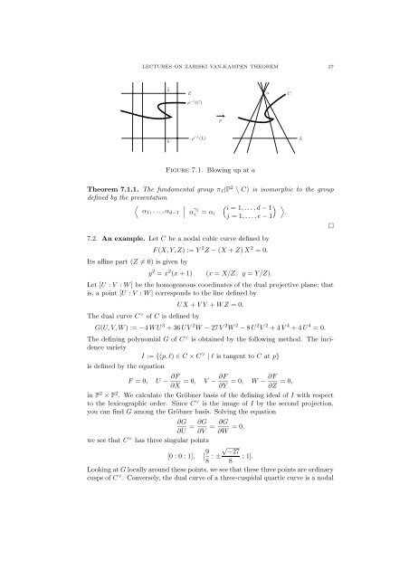
Figure 7.<strong>1.</strong> Blowing up at a<br />
Theorem 7.<strong>1.</strong><strong>1.</strong> The fundamental group π 1 (P 2 \ C) is isomorphic to the group<br />
defined by the presentation<br />
〈 ∣ ( ) 〉<br />
α1 ,...,α ∣∣ γ d−1 α<br />
j i =1,...,d− 1<br />
i = α i .<br />
j =1,...,e− 1<br />
7.2. An example. Let C be a nodal cubic curve defined by<br />
F (X, Y, Z) :=Y 2 Z − (X + Z) X 2 =0.<br />
Its affine part (Z ≠ 0) is given by<br />
y 2 = x 2 (x +1) (x = X/Z, y = Y/Z).<br />
Let [U : V : W ] be the homogeneous coordinates of the dual projective plane; that<br />
is, a point [U : V : W ] corresponds to the line defined by<br />
UX + VY + WZ =0.<br />
The dual curve C ∨ of C is defined by<br />
G(U, V, W ):=−4 WU 3 +36UV 2 W − 27 V 2 W 2 − 8 U 2 V 2 +4V 4 +4U 4 =0.<br />
The defining polynomial G of C ∨ is obtained by the following method. The incidence<br />
variety<br />
I := {(p, l) ∈ C × C ∨ | l is tangent to C at p}<br />
is defined by the equation<br />
F =0, U − ∂F<br />
∂X =0, V − ∂F<br />
∂Y =0, W − ∂F<br />
∂Z =0,<br />
in P 2 × P 2 . We calculate the Gröbner basis of the defining ideal of I with respect<br />
to the lexicographic order. Since C ∨ is the image of I by the second projection,<br />
you can find G among the Gröbner basis. Solving the equation<br />
∂G<br />
∂U = ∂G<br />
∂V = ∂G<br />
∂W =0,<br />
we see that C ∨ has three singular points<br />
[0 : 0 : 1], [ 9 √ −27<br />
8 : ± :1].<br />
8<br />
Looking at G locally around these points, we see that these three points are ordinary<br />
cusps of C ∨ . Conversely, the dual curve of a three-cuspidal quartic curve is a nodal