MATH1725 Introduction to Statistics: Worked examples
MATH1725 Introduction to Statistics: Worked examples
MATH1725 Introduction to Statistics: Worked examples

Create successful ePaper yourself
Turn your PDF publications into a flip-book with our unique Google optimized e-Paper software.
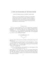
<strong>MATH1725</strong> <strong>Introduction</strong> <strong>to</strong> <strong>Statistics</strong>: <strong>Worked</strong> <strong>examples</strong><br />
<strong>Worked</strong> Example: Lectures 1–2<br />
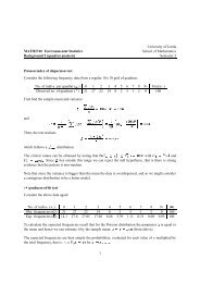
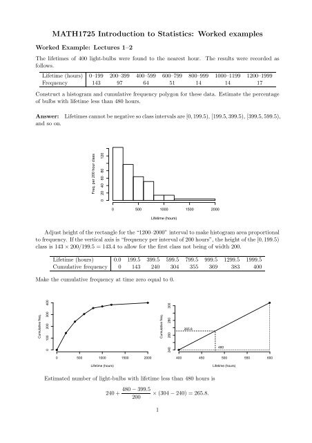
The lifetimes of 400 light-bulbs were found <strong>to</strong> the nearest hour. The results were recorded as<br />
follows.<br />
Lifetime (hours) 0–199 200–399 400–599 600–799 800–999 1000–1199 1200–1999<br />
Frequency 143 97 64 51 14 14 17<br />
Construct a his<strong>to</strong>gram and cumulative frequency polygon for these data. Estimate the percentage<br />
of bulbs with lifetime less than 480 hours.<br />
Answer: Lifetimes cannot be negative so class intervals are [0,199.5), [199.5,399.5), [399.5,599.5),<br />
and so on.<br />
Freq. per 200 hour class<br />
0 20 40 60 80 120<br />
0 500 1000 1500 2000<br />
Lifetime (hours)<br />
Adjust height of the rectangle for the “1200–2000” interval <strong>to</strong> make his<strong>to</strong>gram area proportional<br />
<strong>to</strong> frequency. If the vertical axis is “frequency per interval of 200 hours”, the height of the [0,199.5)<br />
class is 143 × 200/199.5 = 143.4 <strong>to</strong> allow for the first class not being of width 200.<br />
Lifetime (hours) 0.0 199.5 399.5 599.5 799.5 999.5 1299.5 1999.5<br />
Cumulative frequency 0 143 240 304 355 369 383 400<br />
Make the cumulative frequency at time zero equal <strong>to</strong> 0.<br />
Cumulative freq.<br />
0 100 200 300 400<br />
Cumulative freq.<br />
240 260 280 300<br />
265.8<br />
480<br />
0 500 1000 1500 2000<br />
Lifetime (hours)<br />
400 450 500 550 600<br />
Lifetime (hours)<br />
Estimated number of light-bulbs with lifetime less than 480 hours is<br />
240 +<br />
480 − 399.5<br />
200<br />
× (304 − 240) = 265.8.<br />
1
Required percentage is<br />
265.8<br />
400<br />
× 100 = 66.4%<br />
<strong>Worked</strong> Example: Lectures 1–2<br />
The Christmas cactus Zygocactus truncatus has branches made up of separate segments. For one<br />
such cactus the number of segments in each branch were counted.<br />
Number x of segments 1 2 3 4 5 6 7 8 9<br />
Number of branches with x segments 3 0 6 7 8 18 8 0 2<br />
Construct a cumulative frequency polygon <strong>to</strong> represent these data.<br />
Answer: The data is discrete so cumulative frequency plot is a step function.<br />
Number x of segments 1 2 3 4 5 6 7 8 9<br />
Number of branches with ≤ x segments 3 3 9 16 24 42 50 50 52<br />
Cumulative freq.<br />
0 10 20 30 40 50 60<br />
0 2 4 6 8 10<br />
Number of segments<br />
<strong>Worked</strong> Example: Lectures 1–2<br />
The following data give one hundred measurement errors made during the mapping of the American<br />
state of Massachusetts during the last century.<br />
Error X (in minutes ′ of arc) (−4, −2] (−2,0] (0,+2] (+2,+4] (+4,+6]<br />
Frequency 10 43 39 5 3<br />
Show that the sample mean and sample standard deviation for these data are ¯x = −0.04 ′ and<br />
s = 1.717 ′ respectively.<br />
Answer:<br />
Class Class frequency f Class mid-point x fx fx 2<br />
−4< x ≤−2 10 −3 −30 90<br />
−2< x ≤ 0 43 −1 −43 43<br />
0< x ≤+2 39 +1 39 39<br />
+2< x ≤+4 5 +3 15 45<br />
+4< x ≤+6 3 +5 15 75<br />
Totals n = 100 −4 292<br />
2
¯x = −4<br />
100 = −0.04′ .<br />
s 2 = 1 99 (292 − 100 × (−0.04)) = 2.9479, so s = √ (s 2 ) = √ 2.9479 = 1.717 ′ .<br />
<strong>Worked</strong> Example: Lectures 1–2<br />
The time between arrival of 60 patients at an intensive care unit were recorded <strong>to</strong> the nearest hour.<br />
The data are shown below.<br />
Time (hours) 0–19 20–39 40–59 60–79 80–99 100–119 120–139 140–159 160–179<br />
Frequency 16 13 17 4 4 3 1 1 1<br />
Determine the median and semi-interquartile range. Explain why this pair of statistics might be<br />
preferred <strong>to</strong> the mean and standard deviation for these data.<br />
Answer:<br />
Time (hours) 0.0 19.5 39.5 59.5 79.5 99.5 119.5 139.5 159.5 179.5<br />
Cumulative frequency 0 16 29 46 50 54 57 58 59 60<br />
Median lies in “40–59” class, corresponding <strong>to</strong> cumulative frequency 30.<br />
Lower quartile is in “0–19” class, corresponding <strong>to</strong> cumulative frequency 15. Notice that this<br />
class has width 19.5 hours, not 20 hours.<br />
Upper quartile is in “40–59” class, corresponding <strong>to</strong> cumulative frequency 45.<br />
Median = 39.5 +<br />
30 − 29<br />
× 20 = 40.7 hours.<br />
46 − 29<br />
Lower quartile = 0.0 + 15 − 0 × 19.5 = 18.3 hours.<br />
16 − 0<br />
45 − 29<br />
Upper quartile = 39.5 + × 20 = 58.3 hours.<br />
46 − 29<br />
Semi-interquartile range = 1 (58.3 − 18.3) = 20.0 hours.<br />
2<br />
The his<strong>to</strong>gram for these data is positively skew, so the median and semi-interquartile range might<br />
be preferred <strong>to</strong> the mean and standard deviation as measures of location and dispersion respectively.<br />
Freq. per 20 hour class<br />
0 5 10 15 20<br />
0 50 100 150 200<br />
Inter−arrival time (hours)<br />
3
<strong>Worked</strong> Example: Lectures 4–6<br />
A firm investigates the length of telephone conversations of their office staff. Ten consecutive<br />
conversations had lengths, in minutes:<br />
10.7, 9.5, 11.1, 7.8, 11.9, 4.1, 10.0, 9.2, 6.5, 9.2.<br />
Derive a 95% confidence interval for the mean conversation length. Test whether the mean length<br />
of a conversation is eight minutes.<br />
Answer:<br />
¯x = 1 n∑<br />
x i = 90<br />
n 10 = 9 minutes.<br />
i=1<br />
{ n∑<br />
}<br />
s 2 = 1 x 2 i<br />
n − 1<br />
− n¯x2 = 5.42.<br />
i=1<br />
Estimate the population variance σ 2 by s 2 with s = √ 5.42 = 2.33. Then<br />
¯X − µ<br />
s/ √ n ∼ t n−1.<br />
95% confidence interval for µ is ¯x ± t 9 (2.5%)s/ √ 10. Here s/ √ 10 = 0.737, t 9 (2.5%) = 2.262.<br />
s<br />
¯x ± t 9 (2.5%) √ = 9 ± (2.262 × 0.737)<br />
10<br />
= 9 ± 1.667 = (7.3,10.7).<br />
Since 8 minutes lies inside the 95% confidence interval we would accept H 0 in testing H 0 : µ =<br />
8 vs. H 1 : µ ≠ 8 at the 5% significance level.<br />
<strong>Worked</strong> Example: Lectures 5–6<br />
A population has a Poisson distribution but it is not known whether the mean µ is 1 or 4. To<br />
test the hypothesis H 0 : µ = 1 vs. H 1 : µ = 1 on the basis of one observation X the following test<br />
procedure is considered: reject H 0 if X ≥ i.<br />
Type I error is defined <strong>to</strong> be “rejecting H 0 when H 0 is true”. Find the probability of type I<br />
error for the three cases i = 2, 3, 4.<br />
Answer: If H 0 is true, µ = 1 and<br />
so that pr{Type I error} = pr{X ≥ i}.<br />
If i = 2,<br />
pr{X = x} = e−1<br />
x! , x = 0,1,2,... ,<br />
pr{Type I error} = pr{X ≥ 2} = 1−pr{X < 2} = 1−pr{X = 0}−pr{X = 1} = 1−e −1 −e −1 = 0.264.<br />
Similarly if i = 3,<br />
If i = 4,<br />
pr{Type I error} = pr{X ≥ 3} = 1 − pr{X < 3} = 0.080.<br />
pr{Type I error} = pr{X ≥ 4} = 0.019.<br />
Notice that an exact 5% or 10% significance level test does not exist for this discrete distribution.<br />
4
<strong>Worked</strong> Example: Lectures 5–6<br />
A sample of size 64 is drawn by simple random sampling from a normal population which has<br />
known variance 4. The sample mean is −0.45. Test the hypothesis H 0 : µ = 0 vs. H 1 : µ ≠ 0 at<br />
the 5% level of significance. Repeat for testing H 0 : µ = 0 vs. H 1 : µ > 0<br />
Answer: Here ¯X ∼ N(µ,σ 2 /n) with σ 2 = 4, n = 64, so σ 2 /n = 0.0625 and ¯X ∼ N(µ,0.0625).<br />
Test statistic is<br />
Z = ¯X − µ<br />
σ/ √ n = ¯X<br />
√ =<br />
¯X<br />
0.0625 0.25<br />
where Z ∼ N(0,1) if H 0 is true.<br />
For α = 0.05 with a two-sided test, z α/2 = 1.96. Critical region is Z < −1.96 and Z > 1.96.<br />
Observed value is z = −0.45/0.25 = −1.8. This does not lie in critical region so accept H 0 .<br />
For α = 0.05 with a one-sided test, z α = 1.645. Critical region is Z < −1.645. Observed value<br />
is z = −1.8 which lies in critical region so reject H 0 .<br />
<strong>Worked</strong> Example: Lecture 6<br />
The absenteeism rates (in days and parts of days) for nine employees of a large company were<br />
recorded in two consecutive years.<br />
Employee 1 2 3 4 5 6 7 8 9<br />
Year 1 3.0 6.7 11.3 5.0 9.4 15.7 8.0 10.0 9.7<br />
Year 2 2.8 5.1 8.4 5.0 6.2 12.2 10.0 6.8 6.0<br />
Is there any evidence that the average absenteeism rate is different for the two years<br />
Answer: Data paired as same employee studied in each of the two years.<br />
Form difference d i = (year 1) i − (year 2) i . Need <strong>to</strong> estimate variance σ 2 d .<br />
Test H 0 : µ d = 0 vs. H 1 : µ d ≠ 0. See lecture 6.<br />
<strong>Worked</strong> Example: Lecture 8<br />
Which phrases i-iv below apply <strong>to</strong> the sample correlation coefficient r XY <br />
(i) measures linear association between two variables,<br />
(ii) is never negative,<br />
(iii) has positive slope,<br />
(iv) depends on the units of measurement of X and Y .<br />
Answer: i only.<br />
<strong>Worked</strong> Example: Lecture 8<br />
The tensile strength of a glued joint is related <strong>to</strong> the glue thickness. A sample of six values gave<br />
the following results:<br />
Glue Thickness (inches) 0.12 0.12 0.13 0.13 0.14 0.14<br />
Tensile Strength (lbs.) 49.8 46.1 46.5 45.8 44.3 45.9<br />
Calculate the sample correlation coefficient r for these data.<br />
Use the fitted least squares regression line <strong>to</strong> predict the tensile strength of a joint for a glue<br />
thickness of 0.14 inches.<br />
Using scatter-diagrams, sketch the form of regression line expected in the three cases when r<br />
takes the values −1, 0, and +1.<br />
5
Answer: Let X denote the glue thickness and Y the joint strength.<br />
x y x 2 y 2 xy<br />
0.12 49.8 0.0144 2480.04 5.976<br />
0.12 46.1 0.0144 2125.21 5.532<br />
0.13 46.5 0.0169 2162.25 6.045<br />
0.13 45.8 0.0169 2097.64 5.954<br />
0.14 44.3 0.0196 1962.49 6.202<br />
0.14 45.9 0.0196 2106.81 6.426<br />
Totals 0.78 278.4 0.1018 12934.44 36.135<br />
¯x = 0.78<br />
6<br />
= 0.131, ȳ = 278.4<br />
6<br />
= 46.41, s 2 X = 1 5 {0.1018 − 6(0.131)2 } = 0.00008,<br />
s 2 Y = 1 5 {12934.44 − 6(46.41)2 } = 3.336,<br />
s XY = 1 {36.135 − 6(0.131)(46.41)} = −0.0114.<br />
5<br />
Regression line:<br />
r XY = s XY<br />
s X s Y<br />
=<br />
−0.0114<br />
√ 0.00008 × 3.336<br />
= −0.698.<br />
y = ȳ + (x − ¯x) s XY<br />
s 2 X<br />
= 46.4 + (x − 0.13) −0.0114<br />
0.00008<br />
= 64.925 − 142.5x.<br />
At x = 1.4 ′′ this gives y = 44.975 lbs..<br />
Scatter-plots:<br />
r = −1: data lies on a straight line with negative slope.<br />
r = +1: data lies on a straight line with positive slope.<br />
r = 0: data randomly scattered (X and Y independent) or could show case with X and Y having<br />
a non-linear dependence as in the lecture notes. You could even show both of these cases!<br />
<strong>Worked</strong> Example: Lecture 11<br />
A coin is <strong>to</strong>ssed three times. Let X denote the number of heads and Y the length of the longest<br />
run of heads or tails. Thus HTT gives X = 1 and Y = 2, THT gives X = 1 and Y = 1.<br />
(a) Obtain the joint probabilities of X and Y .<br />
(b) Obtain the marginal probability distribution of X and Y .<br />
(c) If X = 1, what is the distribution of Y <br />
Answer: (a and b) All eight outcomes are equally likely, so occur with probability 1/8.<br />
Outcome HHH HHT HTH HTT THH THT TTH TTT<br />
X 3 2 2 1 2 1 1 0<br />
Y 3 2 1 2 2 1 2 3<br />
Probability 1/8 1/8 1/8 1/8 1/8 1/8 1/8 1/8<br />
Y<br />
1 2 3 p X (x)<br />
0 0 0 1/8 1/8<br />
X 1 1/8 1/4 0 3/8<br />
2 1/8 1/4 0 3/8<br />
3 0 0 1/8 1/8<br />
p Y (y) 1/4 1/2 1/4 Total = 1<br />
6
Joint probabilities p(x,y) are found by summing probabilities for each outcome giving rise <strong>to</strong><br />
(X = x,Y = y). Thus p(1,2) = pr{HTT or TTH} = 1/4.<br />
Marginal probabilities are found by forming row or column sum. For example<br />
pr{X = 2} = p(2,1) + p(2,2) + p(2,3) = 3 8 .<br />
(c) If X = 1, then<br />
pr{Y = y|X = 1} = p(1,y)<br />
p X (1) = p(1,y)<br />
3/8 .<br />
Thus<br />
pr{Y = 1|X = 1} = 1/8<br />
2/8<br />
= 1/3, pr{Y = 2|X = 1} = = 2/3, pr{Y = 3|X = 1} = 0.<br />
3/8 3/8<br />
If X = 1, then the outcome is one of HTT, THT, TTH. In one out of these three cases we observe<br />
Y = 1 and in two out of three we observe Y = 2.<br />
<strong>Worked</strong> Example: Lecture 11<br />
Suppose X and Y are independent continuous random variables which are each uniformly distributed<br />
on the interval (0,1).<br />
(a) Find the probability that 0 < X + Y < z for values z ∈ (0,2).<br />
(b) If Z = X + Y , deduce the form of the probability density function f(z) of Z.<br />
Hints: In (a), think about the area on the x-y plane corresponding <strong>to</strong> 0 < x + y < z. In (b), first<br />
find the cumulative distribution function F(z) = pr{Z ≤ z}.<br />
Answer: As X and Y are uniformly distributed on the interval [0,1) they have pdf<br />
f X (x) =<br />
{ 1 if 0 < x < 1,<br />
0 otherwise,<br />
f Y (y) =<br />
{ 1 if 0 < y < 1,<br />
0 otherwise.<br />
(a)<br />
Joint probability density is f(x,y) = f X (x)f Y (y)<br />
by independence of X and Y . Hence f(x,y) = 1,<br />
a constant, for 0 < x < 1 and 0 < y < 1.<br />
1<br />
f(x,y)<br />
Probability of an event A is volume under pdf<br />
with base area given by A. Here A is the region<br />
for which 0 < X + Y < z.<br />
0<br />
A<br />
1<br />
Y<br />
Consider the two cases z < 1 and z > 1 separately.<br />
1<br />
X<br />
Y<br />
1<br />
Case z < 1 Y Case z > 1<br />
1<br />
z<br />
2-z<br />
x+y
{ 1<br />
From the figure above, pr{0 < X + Y < z} = 2 z2 if 0 < z < 1,<br />
1 − 1 2 (2 − z)2 if 1 ≤ z < 2.<br />
An alternative derivation uses integration. For example, in the case z < 1,<br />
∫ ∫<br />
∫ z<br />
∫ z−y<br />
∫ z<br />
pr{0 < X + Y < z} = f(x,y)dxdy = dxdy = (z − y)dy = 1 2 z2 .<br />
0
Answer:<br />
E[T] = E[a 1 X 1 + a 2 X 2 ] = a 1 E[X 1 ] + a 2 E[X 2 ] = a 1 µ + a 2 µ = (a 1 + a 2 )µ.<br />
If we require E[T] = µ, then a 1 + a 2 = 1, so that a 2 = 1 − a 1 .<br />
Since E[T] = µ, then T is said <strong>to</strong> be an unbiased estima<strong>to</strong>r of the mean µ.<br />
Var[T] = Var[a 1 X 1 + a 2 X 2 ] = a 2 1 Var[X 1] + a 2 2 Var[X 2] = a 2 1 σ2 + a 2 2 σ2 = (a 2 1 + a2 2 )σ2 .<br />
Since a 2 = 1 − a 1 , Var[T] = {a 2 1 + (1 − a 1) 2 }σ 2 = (2a 2 1 − 2a 1 + 1)σ 2 . Differentiate this with respect<br />
<strong>to</strong> a 1 <strong>to</strong> find the minimum.<br />
d<br />
da 1<br />
Var[T] = (4a 1 − 2)σ 2 ,<br />
which is zero when a 1 = 1 2 . Hence Var[T] is a minimum when a 1 = a 2 = 1 2 so T = 1 2 (X 1 + X 2 ).<br />
Alternative derivation: write a 1 = 1 2 + ε, a 2 = 1 2<br />
− ε. Then<br />
and is a minimum if ε = 0.<br />
Var[T] = (a 2 1 + a2 2 )σ2 = {( 1 2 + ε)2 + ( 1 2 − ε)2 }σ 2 = ( 1 2 + 2ε2 )σ 2 ,<br />
What does this question show In part (a) you chose a 2 <strong>to</strong> restrict attention <strong>to</strong> linear combinations<br />
of the X i which were unbiased estima<strong>to</strong>rs of the mean µ, so E[T] = µ. In part (b) you then<br />
showed that of all such unbiased estima<strong>to</strong>rs, the sample mean ¯X is the one with smallest variance,<br />
so giving values closest <strong>to</strong> the true mean µ.<br />
<strong>Worked</strong> Example: Lecture 15.<br />
The following data give the noise level (in decibels) generated by fourteen different chain saws<br />
powered in one of two different ways.<br />
Petrol-powered chain saws 103 103 105 106 108 105 106<br />
Electric-powered chain saws 97 95 94 93 91 95 94<br />
At the 5% level of significance, test whether the average noise level of petrol-powered chain saws<br />
is higher than for electric-powered chain saws.<br />
Answer: Testing H 0 : µ 1 = µ 2 vs. H 1 : µ 1 > µ 2 , i.e. H 0 : µ 1 − µ 2 = 0 vs. H 1 : µ 1 − µ 2 > 0.<br />
Have two independent samples with unknown variance. Need <strong>to</strong> assume variances are equal.<br />
<strong>Worked</strong> Example: Lecture 15.<br />
The following data give the length (in mm.) of cuckoo (cuculus canorus) eggs found in nests<br />
belonging <strong>to</strong> wrens (A) and reed warblers (B).<br />
A: 19.8 22.1 21.5 20.9 22.0 21.0 22.3 21.0 20.3 20.9<br />
B: 23.2 22.0 22.2 21.2 21.6 21.6 21.9 22.0 22.9 22.8<br />
Assuming the variances for each group are the same, is there any evidence at the 5% level <strong>to</strong><br />
suggest that the egg size differs between the two host species<br />
9
Answer: Have two independent normal distributions with unknown variances.<br />
Wrens: ¯x 1 = 21.18 mm., s 2 1 = 0.6418, n 1 = 10.<br />
Reed warblers: ¯x 2 = 22.14 mm., s 2 2 = 0.4116, n 2 = 10.<br />
Assume σ 2 1 = σ2 2 = σ2 (unknown). Estimate σ 2 using<br />
s 2 = (n 1 − 1)s 2 1 + (n 2 − 1)s 2 2<br />
= 9s2 1 + 9s2 2<br />
= 0.5267.<br />
n 1 + n 2 − 2 18<br />
( 1<br />
Also ¯x 1 − ¯x 2 = 21.18 − 22.14 = −0.96,<br />
√s 2 + 1 )<br />
= 0.1053, t 18 (2.5%) = 2.101.<br />
n 1 n 2<br />
If µ 1 = µ 2 then the two groups of eggs have the same mean length.<br />
¯x 1 − ¯x 2<br />
To test H 0 : µ 1 = µ 2 vs. H 1 : µ 1 ≠ µ 2 at 5% level, reject H 0 if<br />
√ ∣ s 2 (1/n 1 + 1/n 2 ) ∣ ≥ t 8(2.5%).<br />
¯x 1 − ¯x ∣ ∣<br />
2<br />
∣∣∣<br />
Here<br />
√ ∣ s 2 (1/n 1 + 1/n 2 ) ∣ = −0.96 ∣∣∣<br />
√ = 2.95 so reject the null hypothesis of equal means at 5%<br />
0.1052<br />
level. The two groups of eggs are significantly different at 5% level.<br />
This does not necessarily imply cuckoos can control their egg size. It has been proposed that a<br />
cuckoo lays its egg in the particular nest for which it is best adapted. For further information see:<br />
Wyllie, I. (1981) The Cuckoo. Batsford: London.<br />
Davies, N.B. and Brooke, M. Coevolution of the cuckoo and its host, Scientific American, January<br />
1991, p.66-73.<br />
10
Question (lecture 1-2).<br />
For values 1, 3, 4, 5, 6 obtain the sample mean, sample median, sample variance and sample<br />
standard deviation.<br />
Answer: 1<br />
Question (lecture 1-2).<br />
The number of insurance policies sold by a small firm per week is 7, 8, 5, 6, 6, 7, 9, 5, 7, 8, 4, 7, 6,<br />
7, 7, 5, 8, 6, 7, 6, 6. Obtain the sample mean, sample median, sample variance, sample standard<br />
deviation. Check your values using R.<br />
Answer: 2<br />
Question (lecture 3).<br />
For Z ∼ N(0,1), calculate pr{Z ≤ 0.55}, pr{Z > 2.25}, pr{Z ≤ −0.15}, pr{−1.50 < Z ≤ 2.25}.<br />
Answer: 3<br />
Question (lecture 3).<br />
For Z ∼ N(0,1), calculate pr{Z ≤ 0.63}.<br />
Answer: 4<br />
Question (lecture 3).<br />
For Z ∼ N(0,1), determine the value of z such that: pr{Z ≤ z} = 0.8944, pr{Z > −z} = 0.9713,<br />
pr{−z < Z ≤ z} = 0.9108.<br />
Answer: 5<br />
Question (lecture 3).<br />
An advertising company requires all of its job applicants <strong>to</strong> take a psychometric test. Based on<br />
recent studies, it is believed that the test score follows a normal distribution with mean 100 and<br />
standard deviation 15. Determine the probability that a job applicant will receive a test score<br />
below 118, above 112, between 100 and 112.<br />
Answer: 6<br />
Question (lecture 4).<br />
If X ∼ t 5 , for what value of x is pr{X > x} = 0.05<br />
Answer: 7<br />
Question (lecture 4).<br />
If T ∼ t 8 , for what value t is pr{T > t} = 0.025 For what value t is pr{T ≤ t} = 0.05<br />
Answer: 8<br />
Question (lecture 4).<br />
1 3.8, 4, 3.7, 1.92.<br />
2 6.524, 7.0 (middle ordered value), 1.462, 1.209.<br />
3 pr{Z ≤ 0.55} = Φ(0.55) = 0.7088, pr{Z > 2.25} = 1 − Φ(Z ≤ 2.25) = 1 − Φ(2.25) = 0.0122, pr{Z ≤ −0.15} =<br />
1 − pr{Z ≤ 0.15} = 1 − Φ(0.15) = 0.4404, pr{−1.50 < Z ≤ 2.25} = pr{Z ≤ 2.25} − pr{Z ≤ −1.50} = 0.9210. Recall<br />
that pr{Z > z} = 1 − pr{Z ≤ z}, pr{Z < −z} = pr{Z > z} by symmetry, and also pr{X < b} = pr{X < a} +<br />
pr{a < X < b}.<br />
4 Using interpolation in the tables Φ(0.63) = 0.7356.<br />
5 pr{Z ≤ 1.25} = 0.8944, pr{Z > −1.90} = pr{Z ≤ 1.90} = 0.9713, pr{−z < Z ≤ z} = Φ(z) − Φ(−z) = 2Φ(z) −<br />
1 = 0.9108 so Φ(z) = 0.9554 and z = 1.70.<br />
6 0.8849, 0.2119, 0.2881. Hint: If X ∼ N(µ, σ 2 ), then pr{X ≤ x} = Φ ` x−µ<br />
´.<br />
7 σ<br />
From tables, x = 2.015.<br />
8 t 8(2.5%) = 2.306. pr{T > 1.860} = 0.05 so pr{T ≤ −1.860} = 0.05 by symmetry. Thus t = −1.860.<br />
11
If T ∼ t 10 , what is pr{T ≤ −2.228} What is pr{−2.228 < T ≤ 2.228}<br />
Answer: 9<br />
Question (lecture 4).<br />
If 15, 13, 16, 18, 20 forms a random sample from a normal population with known variance σ 2 = 4,<br />
obtain a 95% confidence interval for the mean µ.<br />
Answer: 10<br />
Question (lecture 4).<br />
A firm investigates the length of time staff spend answering telephone calls. Nine consecutive<br />
conservations had lengths in minutes 10.3, 9.4, 9.9, 7.5, 11.7, 3.4, 7.8, 11.0, 10.0. If these form<br />
a random sample from a normal population with unknown variance σ 2 , obtain a 95% confidence<br />
interval for the mean µ.<br />
Answer: 11<br />
Question (lecture 4).<br />
It is required <strong>to</strong> obtain a 95% confidence interval for the mean µ of a normal population. Previous<br />
work has suggested that the variance σ 2 = 16. How large should the sample size n be if it is<br />
required <strong>to</strong> ensure that the width of the 95% confidence interval for µ is less than 0.5<br />
Answer: 12<br />
Question (lecture 5).<br />
For observations 3, 6, 5, 2 from a normal distribution with mean µ and known variance σ 2 = 4,<br />
test the hypothesis H 0 : µ = 0 against the alternative hypothesis H 1 : µ ≠ 0 at the 5% level.<br />
Answer: 13<br />
Question (lecture 5).<br />
At a gambling establishment I notice that a particular die gives 25 sixes in 100 rolls of the die.<br />
Is the die a fair one (is it biased) (Test whether the probability θ of a six occurring equals 1/6<br />
against the alternative hypothesis that θ ≠ 1/6.)<br />
Answer: 14<br />
Question (lecture 6).<br />
For observations 3, 6, 5, 2 from a normal distribution with mean µ and unknown variance σ 2 , test<br />
the hypothesis H 0 : µ = 1 against the alternative hypothesis H 1 : µ ≠ 1 at the 5% level.<br />
9 0.025, 0.95.<br />
10 n = 5, ¯x = 16.4, 1.96σ/ √ n = 1.753, so 95% interval is 16.4 ± 1.75 = (14.65, 18.15).<br />
11 n = 9, ¯x = 9.0, s 2 = 6.25, t 8(2.5%) = 2.306. Interval is ¯x ± t 8(2.5%) s √ n<br />
= 9.0 ± 1.92.<br />
Rcode which could be used <strong>to</strong> obtain required quantities:<br />
x=c(10.3,9.4,9.9,7.5,11.7,3.4,7.8,11.0,10.0)<br />
mean(x)<br />
var(x)<br />
qt(0.975,8) # Gives 2.5% percentage point for t(8) pdf.<br />
12 Width of interval is 2 × (1.96σ/ √ n). Thus require 2 × (1.96 × 4)/ √ n < 0.5 so n > 16 2 × 1.96 2 = 983.45 so take<br />
n = 984.<br />
13 n = 4, ¯x = 4, σ 2 = 4, µ 0 = 0, σ 2 ¯x − µ0<br />
/n = 1. Test statistic is z =<br />
σ/ √ = 4. Test rule is reject H0 if |z| > 1.96.<br />
n<br />
Thus reject H 0 at 5% level.<br />
14 Let X be number of sixes in 100 throws, so X ∼ Bin(n = 100, θ = 1/6) if H 0 true. X ≈ N(µ = 16.667, σ 2 =<br />
13.889) if H 0 true. Test statistic is z = x √ − 16.667 = 2.236. Test rule is reject H 0 if |z| > 1.96, so reject H 0 at 5%<br />
13.889<br />
level.<br />
12
Answer: 15<br />
Question (lecture 8).<br />
For values (x,y) as given below, obtain the sample correlation r.<br />
Answer: 16<br />
x i 1.1 2.2 3.4 4.5 5.0<br />
y i 3.3 6.1 7.0 10.4 11.5<br />
Question (lecture 10).<br />
For values (x,y) as given below, obtain the line of regression for y given x. What does the residual<br />
at the first data point x 1 = 1.1 equal If x = 4, what is the predicted value of y<br />
Answer: 17<br />
x i 1.1 2.2 3.4 4.5 5.0<br />
y i 3.3 6.1 7.0 10.4 11.5<br />
Question (lecture 10).<br />
For values (x,y) as given below, a line of regression for y given x is fitted.<br />
Test the hypothesis that the slope β equals zero.<br />
Answer: 18<br />
x i 1.1 2.2 3.4 4.5 5.0<br />
y i 3.3 6.1 7.0 10.4 11.5<br />
Question (lecture 11).<br />
Suppose pr{X = x} = x 10<br />
for x = 1,2,3,4. Check that the probability function is valid (is 0 ≤<br />
pr{X = x} ≤ 1 for all x and does ∑ pr{X = x} = 1). Calculate E[X] and Var[X].<br />
x<br />
15 n = 4, ¯x = 4, s 2 = 3.333, µ 0 = 1, s 2 ¯x − µ0<br />
/n = 0.8333. Test statistic is t =<br />
σ/ √ n = √ 4 − 1 = 3.286. Test rule is<br />
0.8333<br />
reject H 0 if |t| > t 3(2.5%). As t 3(2.5%) = 3.182, reject H 0 at 5% level.<br />
16 ¯x = 3.24, s 2 x = 1 X<br />
(xi − ¯x) 2 = 1 “X<br />
x<br />
2<br />
i − n¯x 2” = 2.593,<br />
n − 1<br />
n − 1<br />
ȳ = 7.66, s 2 y = 1 X<br />
(yi − ȳ) 2 = 1 “X<br />
y<br />
2<br />
i − nȳ 2” = 11.033,<br />
n − 1<br />
n − 1<br />
s xy = 1 X<br />
(xi − ¯x)(y i − ȳ) = 1 “X<br />
xiy i − n¯xȳ”<br />
= 5.2645, r XY = s p xy/ s<br />
n − 1<br />
n − 1<br />
2 xs 2 y = 0.984.<br />
Check your answer using R!<br />
x=c(1.1,2.2,3.4,4.5,5.0) # And setup y similarly.<br />
cor(x,y)<br />
17 ¯x = 3.24, ȳ = 7.66, s 2 x = 2.593, s 2 y = 11.033, s xy = 5.2645. Regression line is y = α + βx where ˆβ = s xy/s 2 x =<br />
2.030, ˆα = ȳ − ˆβ¯x = 1.082 so fitted line is y = 1.082 + 2.030x. If x 1 = 1.1, predict ŷ 1 = 3.315. At x = 1.1, residual<br />
is r 1 = y 1 − ŷ 1 = 3.3 − 3.315 = −0.015. If x = 4, predict y = 9.023. Check your answers using R!<br />
x=c(1.1,2.2,3.4,4.5,5.0) # And setup y similarly.<br />
lm(y∼x) # Gives parameter estimates.<br />
model=lm(y∼x) # S<strong>to</strong>res regression model output as model.<br />
model$residual[1]<br />
r<br />
# First residual value.<br />
18 If H 0: β = 0, then ˆβ/ ˆσ<br />
2<br />
∼ t n−2, where S xx = P r<br />
ˆσ<br />
(x i − ¯x) 2 = (n − 1)s 2 2<br />
x. Here = 0.2105 where<br />
S xx S xx<br />
S xx = (n − 1)s 2 x = 10.372. Thus t = 9.646. t 3(2.5%) = 3.182. As |t| > 3.182, reject H 0 at 5% level. Check<br />
your answers using R!<br />
x=c(1.1,2.2,3.4,4.5,5.0) # And setup y similarly.<br />
model=lm(y∼x)<br />
summary(model) # Can you find your answers in the R output<br />
13
Answer: 19<br />
Question (lecture 12).<br />
Suppose (X,Y ) take values (0,0), (0,1), (1,0), (1,1) with probabilities 0.2, 0.5, 0.2, 0.1 respectively.<br />
Obtain the marginal probabilities for X, and the conditional probabilities for Y given X = 1.<br />
Obtain E[XY ]. Are X and Y independent<br />
Answer: 20<br />
Question (lecture 12).<br />
Suppose f XY (x,y) = 4xy for 0 < x < 1 and 0 < y < 1. Obtain the marginal pdf f X (x). Obtain<br />
E[XY ]. Are X and Y independent<br />
Answer: 21<br />
Question (lecture 13).<br />
The table below gives the joint probability function for (X,Y ).<br />
Y<br />
0 1 2<br />
0 0.1 0.1 0.1<br />
X 1 0.2 0.0 0.2<br />
2 0.1 0.0 0.2<br />
Obtain the marginal probabilities p X (x) and p Y (y) for X and Y . Hence obtain E[X], E[Y ], Var[X],<br />
Var[Y ]. Obtain cov(X,Y ) and corr(X,Y ).<br />
Answer: 22<br />
Question (lecture 14).<br />
If cov(X,Y ) = 0.5 and Var[X] = 2, what is cov(X,X + Y )<br />
Answer: 23<br />
Question (lecture 14).<br />
If cov(X + Y,X − Y ) = 12, Var[X + Y ] = 20 and Var[X − Y ] = 16, obtain σ 2 X = Var[X],<br />
σ 2 Y = Var[Y ], σ XY = cov(X,Y ) and so obtain corr(X,Y ).<br />
Answer: 24<br />
Question (lecture 14).<br />
A fair die is rolled 100 times and the number X of ones and the number Y of twos is counted.<br />
What distribution does X have What distribution does Y have If Z = X + Y is the <strong>to</strong>tal<br />
number of ones or twos in the 100 rolls of the die, what distribution does Z have What is the<br />
variance of X, Y and Z Hence obtain cov(X,Y ) and corr(X,Y ).<br />
Answer: 25<br />
19 Yes, 3, 1.<br />
20 p X(0) = 0.7, p X(1) = 0.3, pr{Y = 0|X = 1} = 2 , pr{Y = 1|X = 1} = pr{X = 1 ∩ Y = 1} /pr{X = 1} = 1 .<br />
3 3<br />
E[XY ] = 0.1. No.<br />
21 f X(x) = R y fXY (x, y)dy = 2x for 0 < x < 1. E[XY ] = 4 . Yes.<br />
22 9<br />
Marginal probabilities for X are 0.3, 0.4, 0.3, and for Y they are 0.4, 0.1, 0.5. E[X] = 1, E[Y ] = 1.1,<br />
Var[X] = 0.6, Var[Y ] = 0.89, cov(X, Y ) = 0.1, corr(X, Y ) = 0.137.<br />
23 Var[X] + cov(X, Y ) = 2.5.<br />
24 σX 2 −σY 2 = 12, σX 2 +2σ XY +σY 2 = 20, σX 2 −2σ XY +σY 2 = 16, so 2σX 2 +2σY 2 = 36 and 4σ XY = 4. Thus σX 2 = 15,<br />
σY 2 = 3, σ XY = 1 and corr(X, Y ) = 1/ √ 45.<br />
25 X ∼ Bin(n = 100, θ = 1 ). Similarly for Y . Z ∼ Bin(100, θ = 1 ). Var[X] = Var[Y ] = 500/36, Var[Z] = 200/9 =<br />
6 3<br />
σX 2 + 2σ XY + σY 2 . Hence cov(X, Y ) = −100/36 so corr(X, Y ) = − 1 . Notice X and Y are not uncorrelated. If you<br />
5<br />
have a lot of ones, you would expect fewer twos!<br />
14
Question (lecture 14).<br />
If Var[X] = 4 and Var[Y ] = 9 and corr(X,Y ) = 0.1, obtain cov(X + 2Y,X − Y ).<br />
Answer: 26<br />
Question (lecture 14).<br />
If X ∼ N(1,9) and Y ∼ N(1,16) and X and Y are independent, what is pr{|X − Y | < 5}<br />
Answer: 27<br />
Question (lecture 14).<br />
Suppose that X 1 ,X 2 ,... ,X n are independent and identically distributed random variables with<br />
common mean E[X i ] = µ and common variance Var[X i ] = σ 2 . Let ¯X denote the mean of the X i<br />
with mean µ and variance σ 2 /n. By writing (X i − ¯X) 2 = ({X i − µ} − { ¯X − µ}) 2 and expanding<br />
the bracket, show that<br />
S 2 = 1 n∑<br />
(X i −<br />
n − 1<br />
¯X) 2<br />
has mean E[S 2 ] = σ 2 .<br />
Answer: 28<br />
i=1<br />
Question (lecture 15).<br />
In January 2011 Durham police reported a “significant increase in road accidents during December<br />
[2010] ...mainly due <strong>to</strong> severe weather”. During December 2010 there were 336 reported collisions,<br />
up from 308 in the previous December. By fitting a suitable model <strong>to</strong> these data, test whether<br />
there is indeed a significant difference in the number of accidents between December 2009 and<br />
December 2010. Source: http://www.bbc.co.uk/news/uk-england-12261462<br />
(This is harder than you would get in the examination – I have not done anything like this in the<br />
module. Use the approximation that if X ∼ Poisson(µ) and µ is large, then X ≈ N(µ,σ 2 = µ).)<br />
Answer: 29<br />
Question (lecture 15).<br />
Two independent samples gave values 3, 6, 5, 2 for sample 1 and 2, 2, 3, 3, 5 for sample 2.<br />
Assuming that the samples come from independent normal distributions with known variances 4<br />
and 1 respectively, test at the 5% level whether the difference in mean equals zero against the<br />
alternative that it does not equal zero.<br />
Answer: 30<br />
26 cov(X, Y ) = corr(X, Y ) × p Var[X]Var[Y ] so cov(X, Y ) = 0.6 and cov(X +2Y, X −Y ) = Var[X]+cov(X, Y ) −<br />
2Var[Y ] = −13.4.<br />
27 X − Y ∼ N(0,25) so we want pr{−5 < X − Y ≤ +5}. pr{X − Y ≤ 5} = Φ(1) = 0.8413 so pr{X − Y > 5} =<br />
0.1587 and answer is 0.6826.<br />
28 Recall that Var[X i] = E[(X i − µ) 2 ] = σ 2 and Var[ ¯X] = E[( ¯X − µ) 2 ] = σ 2 /n. Also notice that ({X i − µ} −<br />
{ ¯X − µ}) 2 = (X i − µ) 2 + ( ¯X − µ) 2 − 2(X i − µ)( ¯X − µ) and P i (Xi − µ) = n( ¯X − µ). Thus P P<br />
i (Xi − ¯X) 2 =<br />
i (Xi − µ)2 − n( ¯X − µ) 2 . Now take expectations.<br />
29 A suitable model is <strong>to</strong> assume accidents occur randomly and independently in time. Assuming a constant level<br />
of car usage we are using a Poisson process model. Thus the number X 1 of accidents in December 2010 satisfies<br />
X 1 ∼ Poisson(µ 1). Similarly the number X 2 of accidents in December 2009 satisfies X 2 ∼ Poisson(µ 2). We want <strong>to</strong><br />
test whether µ 1 = µ 2. For µ i large, X i ≈ N(µ i, µ i) for i = 1,2 independently so X 1 − X 2 ≈ N(µ 1 − µ 2, µ 1 + µ 2).<br />
Thus if H 0 is true, and µ 1 = µ 2 = µ,<br />
X1 − X2<br />
U = √ ≈ N(0,1).<br />
2µ<br />
Assuming the null hypothesis is true, we would estimate µ by ˆµ = 1 (336+308) = 322. Thus, replacing µ by ˆµ = 322<br />
2<br />
we obtain U = 1.103. Since |U| < 1.96, we accept the null hypothesis at the 5% level. The observed increase in<br />
accidents was not significant!<br />
30 n 1 = 4, ¯x 1 = 4, σ1 2 = 4, n 2 = 5, ¯x 2 = 3, σ2 2 = 1. Testing H 0: µ 1 − µ 2 = 0 vs. H 1: µ 1 − µ 2 ≠ 0. Test statistic is<br />
15
Question (lecture 15).<br />
Two independent samples gave values 3, 6, 5, 2 for sample 1 and 2, 2, 3, 3, 5 for sample 2. Assuming<br />
that the samples come from independent normal distributions with common unknown variance σ 2 ,<br />
test at the 5% level whether the difference in mean equals zero against the alternative that it does<br />
not equal zero.<br />
Answer: 31<br />
Question (lecture 15).<br />
Five randomly selected remuneration packages for US oil and gas CEOs in 2008 were (in thousands<br />
of US dollars) 21333, 7294, 6712, 5727, 7087. Five randomly selected remuneration packages for<br />
US health care CEOs in 2008 were (in thousands of dollars) 14262, 8381, 7245, 10211, 1817. Test<br />
at the 5% level whether the difference in mean remuneration equals zero against the alternative<br />
hypothesis that it does not equal zero. You can assume that the two populations have common<br />
(unknown) variance σ 2 .<br />
Answer: 32<br />
Question (lecture 16).<br />
A quarter of insurance claims are incomplete in some way. If you have 250 forms <strong>to</strong> process, what<br />
is the approximate probability that you will find fewer than 50 of them incomplete<br />
Answer: 33<br />
Question (lecture 16).<br />
In n = 100 <strong>to</strong>sses of a coin I obtain X = 72 heads. Obtain an approximate 95% confidence interval<br />
for the probability θ of a head.<br />
Answer: 34<br />
Question (lecture 17).<br />
In December 2010 two analysts suggested several shares as likely <strong>to</strong> rise in 2011. By the end of<br />
Oc<strong>to</strong>ber 2011 one (Neil Woodford) had four out of n 1 = 7 “share tips” showing a rise while the<br />
other (Harry Nummo) had three out of n 2 = 10 “share tips” showing a rise. Test at the 5% level<br />
whether the two success proportions are significantly different.<br />
Answer: 35<br />
z =<br />
¯x1 − ¯x2<br />
q<br />
σ 2 1<br />
n 1<br />
+ σ2 2<br />
= q<br />
4 − 3<br />
4<br />
n 2<br />
4 + 1 5<br />
= 0.913. Test rule is reject H 0 if |z| > 1.96. Thus accept H 0 at 5% level.<br />
31 n 1 = 4, ¯x 1 = 4, s 2 1 = 3.333, n 2 = 5, ¯x 2 = 3, s 2 2 = 1.5, pooled estimate of σ 2 is s 2 = 3s2 1 + 4s 2 2<br />
= 2.2857. Testing<br />
7<br />
¯x1 − ¯x2 4 − 3<br />
H 0: µ 1 − µ 2 = 0 vs. H 1: µ 1 − µ 2 ≠ 0. Test statistic is t = q = q = 0.986. Test rule is<br />
1<br />
s<br />
n 1<br />
+ 1<br />
1<br />
n 2<br />
1.5119 × + 1 4 5<br />
reject H 0 if |t| > t 7(2.5%). As t 7(2.5%) = 2.365, accept H 0 at 5% level.<br />
32 Data source: http://graphicsweb.wsj.com/php/CEOPAY09.html.<br />
n 1 = 5, ¯x 1 = 9630.6, s 2 1 = 43158021, n 2 = 5, ¯x 2 = 8383.2, s 2 2 = 20577907, n 1 + n 2 − 2 = 8, t 8(2.5%) = 2.306.<br />
If variances are equal <strong>to</strong> σ 2 , estimate σ 2 using s 2 = (n1 − 1)s2 1 + (n 2 − 1)s 2 2<br />
= 31867964. Test statistic is t =<br />
n 1 + n 2 − 2<br />
|¯x 1 −¯x 2 |<br />
= 0.349. Since t8(2.5%) = 2.306, then |t| < t8(2.5%) so accept H0 that µ1 = µ2 against the<br />
r<br />
s 2 ( 1<br />
n 1<br />
+ 1<br />
n 2<br />
)<br />
= 1247.4<br />
3570.32<br />
alternative µ 1 ≠ µ 2 at the 5% level.<br />
33 If X is the number of incomplete forms, X ∼ Bin(n = 250, θ = 1 ) ≈ N(µ = 62.5, 4 σ2 = 46.875). You require<br />
„ 49 +<br />
1<br />
2<br />
pr{X < 50} = pr{X ≤ 49} = Φ<br />
− µ «<br />
= Φ(−1.899) = 0.0288. Notice we have used a continuity correction.<br />
σ<br />
34 Number of heads X ∼ Bin(n = 100, θ).<br />
s<br />
Here n = 100, X = 72 observed, ˆθ = X/n = 72/100 = 0.72.<br />
Approximate 95% confidence interval is ˆθ<br />
ˆθ(1 −<br />
± 1.96<br />
ˆθ) = 0.72 ± 0.088.<br />
n<br />
35 Data source: http://www.thisismoney.co.uk/money/investing/article-1709914/S<strong>to</strong>ck-market-predict<br />
16
Question (lecture 17).<br />
In January 2011 Durham police were reported as disappointed by the increase in the number<br />
of people arrested for drinking and driving. Between December 1st 2010 and December<br />
31st 2010 they had 52 positive breath tests out of 1799 breath tests administered, while for<br />
the same period in 2009 they had 41 positive tests out of 1433 administered. Construct a<br />
95% confidence interval for the difference in proportion of drivers who tested positive. Source:<br />
http://www.bbc.co.uk/news/uk-england-12261462<br />
Answer: 36<br />
Question (lecture 17).<br />
I observe two dice. For one die I notice that it gives a six 20 times out of 100 and for the second<br />
die I notice that it gives a six 22 times out of 80. Test at the 5% level whether the two dice give<br />
the same probability of showing a six.<br />
Answer: 37<br />
Question (lecture 18).<br />
If X ∼ χ 2 4 , for what value of x is pr{X > x} = 0.05<br />
Answer: 38<br />
Question (lecture 19).<br />
I roll a die 100 times and observe the following results.<br />
Test at the 5% level whether the die is fair.<br />
Answer: 39<br />
Outcome i 1 2 3 4 5 6<br />
Observed frequency 16 15 16 15 15 23<br />
ions-tips-2011.html<br />
Two binomial proportions here. ˆθ1 = 4/7 = 0.571, ˆθ2 = 3/10 = 0.300, n 1 = 7, n 2 = 10. Common estimated<br />
proportion is θ = 7ˆθ 1 + 10ˆθ 2<br />
|ˆθ 1 −<br />
= 0.412. Approximate test statistic is z =<br />
ˆθ 2|<br />
r<br />
17<br />
ˆθ(1 − ˆθ)<br />
“ = 1.119. reject H0 at<br />
1<br />
n 1<br />
+ 1<br />
5% level if |z| > 1.96, so here accept the hypothesis that the two proportions are equal.<br />
36 Two binomial proportions again. ˆθ 1 = 52/1799 = 0.028905, ˆθ 2 = 41/1433 = 0.028611, n 1 = 1799, n 2 = 1433.<br />
Common estimated proportion is θ = 1799ˆθ 1 + 1433ˆθ 2<br />
= 0.0288. (This is very small so the normal approximation<br />
is doubtful. In practice we would transform <strong>to</strong> give approximate normality.) Approximate test statistic is<br />
3232<br />
|ˆθ 1 −<br />
z =<br />
ˆθ 2|<br />
r<br />
ˆθ(1 − ˆθ)<br />
“ = 0.0496. Reject H0 at 5% level if |z| > 1.96, so here accept the hypothesis that the two<br />
1<br />
n 1<br />
+ 1<br />
n 2<br />
”<br />
proportions are equal.<br />
37 n 1 = 100, x 1 = 20, ˆθ1 = 20/100 = 0.200, n 2 = 80, x 2 = 22, ˆθ2 = 22/80 = 0.275. We test H 0: θ 1 =<br />
θ 2(= θ) vs. H 1: θ 1 ≠ θ 2. This is equivalent <strong>to</strong> testing H 0: θ 1 − θ 2 = 0 vs. H 1: θ 1 − θ 2 ≠ 0. Assuming H 0 is<br />
true, the estimated common proportion θ is estimated by ˆθ = n1ˆθ 1 + n 2ˆθ2<br />
=<br />
n 1 + n 2<br />
ˆθ 1 −<br />
z =<br />
ˆθ 2<br />
q =<br />
ˆθ(1−ˆθ)<br />
+ ˆθ(1−ˆθ)<br />
n 2<br />
n 1<br />
20 + 22<br />
180<br />
n 2<br />
”<br />
= 0.2333. Test statistic is<br />
0.200 − 0.275<br />
√ 0.0017889 + 0.0014907<br />
= −1.31. Test rule is reject H 0 if |z| > 1.96, so accept H 0 at 5%<br />
level.<br />
38 From tables, x = 9.488.<br />
39 Let X denote the outcome of the die. We test whether pr{X = i} = 1/6 for all i. Expected frequency for any<br />
outcome would then be 100 × 1 6 = 16.667.<br />
Outcome i 1 2 3 4 5 6<br />
Observed frequency O i 16 15 16 15 15 23<br />
Expected frequency E i 16.67 16.67 16.67 16.67 16.67 16.67<br />
(O i − E i) 2 /E i 0.0267 0.1667 0.0267 0.1667 0.1667 2.407 sum=2.960<br />
17
Question (lecture 19).<br />
I live 55 miles commuting distance from the University. Over 35 car journeys I count the number<br />
X of road accidents observed and obtain the following data.<br />
Number of accidents observed per journey X 0 1 2<br />
Observed frequency 28 5 2<br />
Test at the 5% level whether a Poisson distribution gives a good fit <strong>to</strong> the data. Why is the Poisson<br />
distribution a suitable model for these data<br />
Answer: 40<br />
Question (lecture 20).<br />
Two surveys were conducted about a certain product and the following results obtained.<br />
Like OK Dislike Total<br />
Survey A 44 23 33 100<br />
Survey B 30 20 30 80<br />
Total 74 43 63 180<br />
Test whether the like/OK/dislike population proportions for the two surveys are equal.<br />
Answer: 41<br />
Number of cells is 6; number of estimated parameters is 0; number of constraints on expected frequencies is 1.<br />
Number of degrees of freedom is k = 6 − 0 − 1 = 5. Test statistic is χ 2 obs = 2.960. Reject H 0 if χ 2 obs > χ 2 5(5%). As<br />
χ 2 5(5%) = 11.071, we accept the null hypothesis that the die is fair.<br />
40 ¯x = 9/35 = 0.257. Best fitting Poisson distribution is X ∼ Poisson(µ = 0.257). Fitted probabilities are<br />
pr{X = x} = µx e −µ<br />
x!<br />
for x = 0,1, 2, . . .. Fitted frequencies are E x = 35 × pr{X = x} for x = 0,1, 2, . . ..<br />
Number of accidents X 0 1 ≥ 2<br />
Observed frequency O i 28 5 2<br />
Expected frequency E i 27.06 6.959 0.977<br />
(by difference)<br />
(O i − E i) 2 /E i 0.0324 0.5516 1.0723 sum=1.656<br />
Number of cells is 3; number of estimated parameters is 1; number of constraints on expected frequencies is 1.<br />
Number of degrees of freedom is k = 3 − 1 − 1 = 1. Test statistic is χ 2 obs = 1.656. Reject H 0 if χ 2 obs > χ 2 1(5%). As<br />
χ 2 1(5%) = 3.841, we accept the Poisson distribution fit.<br />
Poisson distribution sensible model by thinking of a Poisson process. If accidents happen randomly and independently<br />
in time, number in one journey of an hour has a Poisson distribution.<br />
In practice we might pool cells <strong>to</strong> ensure all expected frequencies are at least five. Also for χ 2 -tests with one degree<br />
of freedom a better test uses Yates’s continuity correction so that χ 2 obs = X (|O i − E i| − 1 2 )2<br />
.<br />
E i<br />
i<br />
41 (row <strong>to</strong>tal) × (column <strong>to</strong>tal)<br />
Expected frequencies are . Thus:<br />
grand <strong>to</strong>tal<br />
Like OK Dislike Total<br />
Survey A (100 × 74)/180 = 41.11 23.89 35.00 100<br />
Survey B 32.89 19.11 28.00 80<br />
Total 74 43 63 180<br />
Number of degrees of freedom is k = (3 − 1)(2 − 1) = 2.<br />
(O i − E i) 2 /E i Like OK Dislike<br />
Survey A 0.2030 0.0331 0.1143<br />
Survey B 0.2538 0.0413 0.1429<br />
Test statistic is χ 2 obs = X i<br />
(O i − E i) 2 /E i = 0.7883. Reject H 0 if χ 2 obs > χ 2 2(5%). As χ 2 2(5%) = 5.991, so accept<br />
hypothesis that the two surveys have the same overall proportions for each category.<br />
Note that the test is whether the proportion liking is the same for surveys A and B, and the proportions saying OK<br />
are the same for A and B, and the proportions disliking are the same for A and B.<br />
18