MATH1725 Introduction to Statistics: Worked examples

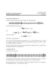
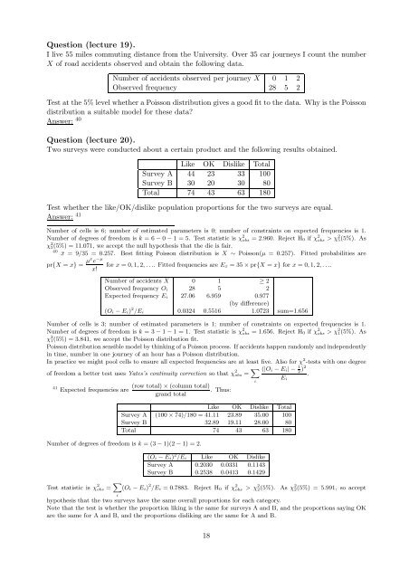
Question (lecture 19).
I live 55 miles commuting distance from the University. Over 35 car journeys I count the number
X of road accidents observed and obtain the following data.
Number of accidents observed per journey X 0 1 2
Observed frequency 28 5 2
Test at the 5% level whether a Poisson distribution gives a good fit to the data. Why is the Poisson
distribution a suitable model for these data
Answer: 40
Question (lecture 20).
Two surveys were conducted about a certain product and the following results obtained.
Like OK Dislike Total
Survey A 44 23 33 100
Survey B 30 20 30 80
Total 74 43 63 180
Test whether the like/OK/dislike population proportions for the two surveys are equal.
Answer: 41
Number of cells is 6; number of estimated parameters is 0; number of constraints on expected frequencies is 1.
Number of degrees of freedom is k = 6 − 0 − 1 = 5. Test statistic is χ 2 obs = 2.960. Reject H 0 if χ 2 obs > χ 2 5(5%). As
χ 2 5(5%) = 11.071, we accept the null hypothesis that the die is fair.
40 ¯x = 9/35 = 0.257. Best fitting Poisson distribution is X ∼ Poisson(µ = 0.257). Fitted probabilities are
pr{X = x} = µx e −µ
x!
for x = 0,1, 2, . . .. Fitted frequencies are E x = 35 × pr{X = x} for x = 0,1, 2, . . ..
Number of accidents X 0 1 ≥ 2
Observed frequency O i 28 5 2
Expected frequency E i 27.06 6.959 0.977
(by difference)
(O i − E i) 2 /E i 0.0324 0.5516 1.0723 sum=1.656
Number of cells is 3; number of estimated parameters is 1; number of constraints on expected frequencies is 1.
Number of degrees of freedom is k = 3 − 1 − 1 = 1. Test statistic is χ 2 obs = 1.656. Reject H 0 if χ 2 obs > χ 2 1(5%). As
χ 2 1(5%) = 3.841, we accept the Poisson distribution fit.
Poisson distribution sensible model by thinking of a Poisson process. If accidents happen randomly and independently
in time, number in one journey of an hour has a Poisson distribution.
In practice we might pool cells to ensure all expected frequencies are at least five. Also for χ 2 -tests with one degree
of freedom a better test uses Yates’s continuity correction so that χ 2 obs = X (|O i − E i| − 1 2 )2
.
E i
i
41 (row total) × (column total)
Expected frequencies are . Thus:
grand total
Like OK Dislike Total
Survey A (100 × 74)/180 = 41.11 23.89 35.00 100
Survey B 32.89 19.11 28.00 80
Total 74 43 63 180
Number of degrees of freedom is k = (3 − 1)(2 − 1) = 2.
(O i − E i) 2 /E i Like OK Dislike
Survey A 0.2030 0.0331 0.1143
Survey B 0.2538 0.0413 0.1429
Test statistic is χ 2 obs = X i
(O i − E i) 2 /E i = 0.7883. Reject H 0 if χ 2 obs > χ 2 2(5%). As χ 2 2(5%) = 5.991, so accept
hypothesis that the two surveys have the same overall proportions for each category.
Note that the test is whether the proportion liking is the same for surveys A and B, and the proportions saying OK
are the same for A and B, and the proportions disliking are the same for A and B.
18