AN INTRODUCTION TO MULTIVARIATE STATISTICS - Ecu

An Introduction to Multivariate Statistics
The term “multivariate statistics” is appropriately used to include all statistics where there are more
than two variables simultaneously analyzed. You are already familiar with bivariate statistics such as the
Pearson product moment correlation coefficient and the independent groups t-test. A one-way ANOVA with 3
or more treatment groups might also be considered a bivariate design, since there are two variables: one
independent variable and one dependent variable. Statistically, one could consider the one-way ANOVA as
either a bivariate curvilinear regression or as a multiple regression with the K level categorical independent
variable dummy coded into K-1 dichotomous variables.
Independent vs. Dependent Variables
We shall generally continue to make use of the terms “independent variable” and “dependent variable,”
but shall find the distinction between the two somewhat blurred in multivariate designs, especially those
observational rather than experimental in nature. Classically, the independent variable is that which is
manipulated by the researcher. With such control, accompanied by control of extraneous variables through
means such as random assignment of subjects to the conditions, one may interpret the correlation between the
dependent variable and the independent variable as resulting from a cause-effect relationship from
independent (cause) to dependent (effect) variable. Whether the data were collected by experimental or
observational means is NOT a consideration in the choice of an analytic tool. Data from an experimental
design can be analyzed with either an ANOVA or a regression analysis (the former being a special case of the
latter) and the results interpreted as representing a cause-effect relationship regardless of which statistic was
employed. Likewise, observational data may be analyzed with either an ANOVA or a regression analysis, and
the results cannot be unambiguously interpreted with respect to causal relationship in either case.
We may sometimes find it more reasonable to refer to “independent variables” as “predictors”, and
“dependent variables” as “response-,” “outcome-,” or “criterion-variables.” For example, we may use SAT
scores and high school GPA as predictor variables when predicting college GPA, even though we wouldn’t
want to say that SAT causes college GPA. In general, the independent variable is that which one considers
the causal variable, the prior variable (temporally prior or just theoretically prior), or the variable on which one
has data from which to make predictions.
Descriptive vs. Inferential Statistics
While psychologists generally think of multivariate statistics in terms of making inferences from a
sample to the population from which that sample was randomly or representatively drawn, sometimes it may
be more reasonable to consider the data that one has as the entire population of interest. In this case, one
may employ multivariate descriptive statistics (for example, a multiple regression to see how well a linear
model fits the data) without worrying about any of the assumptions (such as homoscedasticity and normality of
conditionals or residuals) associated with inferential statistics. That is, multivariate statistics, such as R 2 , can
be used as descriptive statistics. In any case, psychologists rarely ever randomly sample from some
population specified a priori, but often take a sample of convenience and then generalize the results to some
abstract population from which the sample could have been randomly drawn.
Rank-Data
I have mentioned the assumption of normality common to “parametric” inferential statistics. Please
note that ordinal data may be normally distributed and interval data may not, so scale of measurement is
irrelevant. Rank-ordinal data will, however, be non-normally distributed (rectangular), so one might be
concerned about the robustness of a statistic’s normality assumption with rectangular data. Although this is a
Copyright 2013 Karl L. Wuensch - All rights reserved.
Intro.MV.docx

2
controversial issue, I am moderately comfortable with rank data when there are twenty to thirty or more ranks
in the sample (or in each group within the total sample).
Why (and Why Not) Should One Use Multivariate Statistics
One might object that psychologists got along OK for years without multivariate statistics. Why the
sudden surge of interest in multivariate stats Is it just another fad Maybe it is. There certainly do remain
questions that can be well answered with simpler statistics, especially if the data were experimentally
generated under controlled conditions. But many interesting research questions are so complex that they
demand multivariate models and multivariate statistics. And with the greatly increased availability of high
speed computers and multivariate software, these questions can now be approached by many users via
multivariate techniques formerly available only to very few. There is also an increased interest recently with
observational and quasi-experimental research methods. Some argue that multivariate analyses, such as
ANCOV and multiple regression, can be used to provide statistical control of extraneous variables. While I
opine that statistical control is a poor substitute for a good experimental design, in some situations it may be
the only reasonable solution. Sometimes data arrive before the research is designed, sometimes experimental
or laboratory control is unethical or prohibitively expensive, and sometimes somebody else was just plain
sloppy in collecting data from which you still hope to distill some extract of truth.
But there is danger in all this. It often seems much too easy to find whatever you wish to find in any
data using various multivariate fishing trips. Even within one general type of multivariate analysis, such as
multiple regression or factor analysis, there may be such a variety of “ways to go” that two analyzers may
easily reach quite different conclusions when independently analyzing the same data. And one analyzer may
select the means that maximize e’s chances of finding what e wants to find or e may analyze the data many
different ways and choose to report only that analysis that seems to support e’s a priori expectations (which
may be no more specific than a desire to find something “significant,” that is, publishable). Bias against the
null hypothesis is very great.
It is relatively easy to learn how to get a computer to do multivariate analysis. It is not so easy correctly
to interpret the output of multivariate software packages. Many users doubtlessly misinterpret such output, and
many consumers (readers of research reports) are being fed misinformation. I hope to make each of you a
more critical consumer of multivariate research and a novice producer of such. I fully recognize that our
computer can produce multivariate analyses that cannot be interpreted even by very sophisticated persons.
Our perceptual world is three dimensional, and many of us are more comfortable in two dimensional space.
Multivariate statistics may take us into hyperspace, a space quite different from that in which our brains (and
thus our cognitive faculties) evolved.
Categorical Variables and LOG LINEAR ANALYSIS
We shall consider multivariate extensions of statistics for designs where we treat all of the variables as
categorical. You are already familiar with the bivariate (two-way) Pearson Chi-square analysis of contingency
tables. One can expand this analysis into 3 dimensional space and beyond, but the log-linear model covered
in Chapter 17 of Howell is usually used for such multivariate analysis of categorical data. As a example of
such an analysis consider the analysis reported by Moore, Wuensch, Hedges, & Castellow in the Journal of
Social Behavior and Personality, 1994, 9: 715-730. In the first experiment reported in this study mock jurors
were presented with a civil case in which the female plaintiff alleged that the male defendant had sexually
harassed her. The manipulated independent variables were the physical attractiveness of the defendant
(attractive or not), and the social desirability of the defendant (he was described in the one condition as being
socially desirable, that is, professional, fair, diligent, motivated, personable, etc., and in the other condition as
being socially undesirable, that is, unfriendly, uncaring, lazy, dishonest, etc.) A third categorical independent
variable was the gender of the mock juror. One of the dependent variables was also categorical, the verdict
rendered (guilty or not guilty). When all of the variables are categorical, log-linear analysis is appropriate.
When it is reasonable to consider one of the variables as dependent and the others as independent, as in this
study, a special type of log-linear analysis called a LOGIT ANALYSIS is employed. In the second experiment
in this study the physical attractiveness and social desirability of the plaintiff were manipulated.

Earlier research in these authors’ laboratory had shown that both the physical attractiveness and the
social desirability of litigants in such cases affect the outcome (the physically attractive and the socially
desirable being more favorably treated by the jurors). When only physical attractiveness was manipulated
(Castellow, Wuensch, & Moore, Journal of Social Behavior and Personality, 1990, 5: 547-562) jurors favored
the attractive litigant, but when asked about personal characteristics they described the physically attractive
litigant as being more socially desirable (kind, warm, intelligent, etc.), despite having no direct evidence about
social desirability. It seems that we just assume that the beautiful are good. Was the effect on judicial
outcome due directly to physical attractiveness or due to the effect of inferred social desirability When only
social desirability was manipulated (Egbert, Moore, Wuensch, & Castellow, Journal of Social Behavior and
Personality, 1992, 7: 569-579) the socially desirable litigants were favored, but jurors rated them as being more
physically attractive than the socially undesirable litigants, despite having never seen them! It seems that we
also infer that the bad are ugly. Was the effect of social desirability on judicial outcome direct or due to the
effect on inferred physical attractiveness The 1994 study attempted to address these questions by
simultaneously manipulating both social desirability and physical attractiveness.
In the first experiment of the 1994 study it was found that the verdict rendered was significantly affected
by the gender of the juror (female jurors more likely to render a guilty verdict), the social desirability of the
defendant (guilty verdicts more likely with socially undesirable defendants), and a strange Gender x Physical
Attractiveness interaction: Female jurors were more likely to find physically attractive defendants guilty, but
male jurors’ verdicts were not significantly affected by the defendant’s physical attractiveness (but there was a
nonsignificant trend for them to be more likely to find the unattractive defendant guilty). Perhaps female jurors
deal more harshly with attractive offenders because they feel that they are using their attractiveness to take
advantage of a woman.
The second experiment in the 1994 study, in which the plaintiff’s physical attractiveness and social
desirability were manipulated, found that only social desirability had a significant effect (guilty verdicts were
more likely when the plaintiff was socially desirable). Measures of the strength of effect ( 2 ) of the
independent variables in both experiments indicated that the effect of social desirability was much greater than
any effect of physical attractiveness, leading to the conclusion that social desirability is the more important
factor—if jurors have no information on social desirability, they infer social desirability from physical
attractiveness and such inferred social desirability affects their verdicts, but when jurors do have relevant
information about social desirability, litigants’ physical attractiveness is of relatively little importance.
3
Continuous Variables
We shall usually deal with multivariate designs in which one or more of the variables is considered to
be continuously distributed. We shall not nit-pick on the distinction between continuous and discrete variables,
as I am prone to do when lecturing on more basic topics in statistics. If a discrete variable has a large number
of values and if changes in these values can be reasonably supposed to be associated with changes in the
magnitudes of some underlying construct of interest, then we shall treat that discrete variable as if it were
continuous. IQ scores provide one good example of such a variable.
CANONICAL CORRELATION/REGRESSION:
Also known as multiple multiple regression or multivariate multiple regression. All other multivariate
techniques may be viewed as simplifications or special cases of this “fully multivariate general linear model.”
We have two sets of variables (set X and set Y). We wish to create a linear combination of the X variables
(b 1 X 1 + b 2 X 2 + .... + b p X p ), called a canonical variate, that is maximally correlated with a linear combination of
the Y variables (a 1 Y 1 + a 2 Y 2 + .... + a q Y q ). The coefficients used to weight the X’s and the Y’s are chosen with
one criterion, maximize the correlation between the two linear combinations.

4
As an example, consider the research reported by Patel, Long, McCammon, & Wuensch (Journal of
Interpersonal Violence, 1995, 10: 354-366). We had two sets of data on a group of male college students.
The one set was personality variables from the MMPI. One of these was the PD (psychopathically deviant)
scale, Scale 4, on which high scores are associated with general social maladjustment and hostility. The
second was the MF (masculinity/femininity) scale, Scale 5, on which low scores are associated with
stereotypical masculinity † . The third was the MA (hypomania) scale, Scale 9, on which high scores are
associated with overactivity, flight of ideas, low frustration tolerance, narcissism, irritability, restlessness,
hostility, and difficulty with controlling impulses. The fourth MMPI variable was Scale K, which is a validity
scale on which high scores indicate that the subject is “clinically defensive,” attempting to present himself in a
favorable light, and low scores indicate that the subject is unusually frank. The second set of variables was a
pair of homonegativity variables. One was the IAH (Index of Attitudes Towards Homosexuals), designed to
measure affective components of homophobia. The second was the SBS, (Self-Report of Behavior Scale),
designed to measure past aggressive behavior towards homosexuals, an instrument specifically developed for
this study.
With luck, we can interpret the weights (or, even better, the loadings, the correlations between each
canonical variable and the variables in its set) so that each of our canonical variates represents some
underlying dimension (that is causing the variance in the observed variables of its set). We may also think of
a canonical variate as a superordinate variable, made up of the more molecular variables in its set. After
constructing the first pair of canonical variates we attempt to construct a second pair that will explain as much
as possible of the (residual) variance in the observed variables, variance not explained by the first pair of
canonical variates. Thus, each canonical variate of the X’s is orthogonal to (independent of) each of the other
canonical variates of the X’s and each canonical variate of the Y’s is orthogonal to each of the other canonical
variates of the Y’s. Construction of canonical variates continues until you can no longer extract a pair of
canonical variates that accounts for a significant proportion of the variance. The maximum number of pairs
possible is the smaller of the number of X variables or number of Y variables.
In the Patel et al. study both of the canonical correlations were significant. The first canonical
correlation indicated that high scores on the SBS and the IAH were associated with stereotypical masculinity
(low Scale 5), frankness (low Scale K), impulsivity (high Scale 9), and general social maladjustment and
hostility (high Scale 4). The second canonical correlation indicated that having a low IAH but high SBS (not
being homophobic but nevertheless aggressing against gays) was associated with being high on Scales 5 (not
being stereotypically masculine) and 9 (impulsivity). The second canonical variate of the homonegativity
variables seems to reflect a general (not directed towards homosexuals) aggressiveness.
MULTIPLE REGRESSION
In a standard multiple regression we have one continuous Y variable and two or more continuous X
variables. Actually, the X variables may include dichotomous variables and/or categorical variables that have
been “dummy coded” into dichotomous variables. The goal is to construct a linear model that minimizes error
in predicting Y. That is, we wish to create a linear combination of the X variables that is maximally correlated
with the Y variable. We obtain standardized regression coefficients ( weights
Z Z Z
Z
Y 1 1 2 2 p p) that represent how large an “effect” each X has on Y above and beyond the
effect of the other X’s in the model. The predictors may be entered all at once (simultaneous) or in sets of one
or more (sequential). We may use some a priori hierarchical structure to build the model sequentially (enter
first X 1 , then X 2 , then X 3 , etc., each time seeing how much adding the new X improves the model, or, start with
all X’s, then first delete X 1 , then delete X 2 , etc., each time seeing how much deletion of an X affects the model).
We may just use a statistical algorithm (one of several sorts of stepwise selection) to build what we hope is
the “best” model using some subset of the total number of X variables available.
For example, I may wish to predict college GPA from high school grades, SATV, SATQ, score on a
“why I want to go to college” essay, and quantified results of an interview with an admissions officer. Since
some of these measures are less expensive than others, I may wish to give them priority for entry into the
model. I might also give more “theoretically important” variables priority. I might also include sex and race as

5
predictors. I can also enter interactions between variables as predictors, for example, SATM x SEX, which
would be literally represented by an X that equals the subject’s SATM score times e’s sex code (typically 0 vs.
1 or 1 vs. 2). I may fit nonlinear models by entering transformed variables such as LOG(SATM) or SAT 2 . We
shall explore lots of such fun stuff later.
As an example of a multiple regression analysis, consider the research reported by McCammon,
Golden, and Wuensch in the Journal of Research in Science Teaching, 1988, 25, 501-510. Subjects were
students in freshman and sophomore level Physics courses (only those courses that were designed for
science majors, no general education courses). The mission was to develop a model to
predict performance in the course. The predictor variables were CT (the Watson-Glaser Critical Thinking
Appraisal), PMA (Thurstone’s Primary Mental Abilities Test), ARI (the College Entrance Exam Board’s
Arithmetic Skills Test), ALG (the College Entrance Exam Board’s Elementary Algebra Skills Test), and ANX
(the Mathematics Anxiety Rating Scale). The criterion variable was subjects’ scores on course examinations.
All of the predictor variables were significantly correlated with one another and with the criterion variable. A
simultaneous multiple regression yielded a multiple R of .40 (which is more impressive if you consider that the
data were collected across several sections of different courses with different instructors). Only ALG and CT
had significant semipartial correlations (indicating that they explained variance in the criterion that was not
explained by any of the other predictors). Both forward and backwards selection analyses produced a
model containing only ALG and CT as predictors. At Susan McCammon’s insistence, I also separately
analyzed the data from female and male students. Much to my surprise I found a remarkable sex difference.
Among female students every one of the predictors was significantly related to the criterion, among male
students none of the predictors was. There were only small differences between the sexes on variance in the
predictors or the criterion, so it was not a case of there not being sufficient variability among the men to support
covariance between their grades and their scores on the predictor variables. A posteriori searching of the
literature revealed that Anastasi (Psychological Testing, 1982) had noted a relatively consistent finding of sex
differences in the predictability of academic grades, possibly due to women being more conforming and more
accepting of academic standards (better students), so that women put maximal effort into their studies,
whether or not they like the course, and according they work up to their potential. Men, on the other hand, may
be more fickle, putting forth maximum effort only if they like the course, thus making it difficult to predict their
performance solely from measures of ability.
LOGISTIC REGRESSION
Logistic regression is used to predict a categorical (usually dichotomous) variable from a set of
predictor variables. With a categorical dependent variable, discriminant function analysis is usually employed if
all of the predictors are continuous and nicely distributed; logit analysis is usually employed if all of the
predictors are categorical; and logistic regression is often chosen if the predictor variables are a mix of
continuous and categorical variables and/or if they are not nicely distributed (logistic regression makes no
assumptions about the distributions of the predictor variables). Logistic regression has been especially popular
with medical research in which the dependent variable is whether or not a patient has a disease.
For a logistic regression, the predicted dependent variable is the estimated probability that a particular
subject will be in one of the categories (for example, the probability that Suzie Cue has the disease, given her
set of scores on the predictor variables).
As an example of the use of logistic regression in psychological research, consider the research done
by Wuensch and Poteat and published in the Journal of Social Behavior and Personality, 1998, 13, 139-150.
College students (N = 315) were asked to pretend that they were serving on a university research committee
hearing a complaint against animal research being conducted by a member of the university faculty. Five
different research scenarios were used: Testing cosmetics, basic psychological theory testing, agricultural
(meat production) research, veterinary research, and medical research. Participants were asked to decide
whether or not the research should be halted. An ethical inventory was used to measure participants’ idealism
(persons who score high on idealism believe that ethical behavior will always lead only to good consequences,
never to bad consequences, and never to a mixture of good and bad consequences) and relativism (persons

6
who score high on relativism reject the notion of universal moral principles, preferring personal and situational
analysis of behavior).
Since the dependent variable was dichotomous (whether or not the respondent decided to halt the
research) and the predictors were a mixture of continuous and categorical variables (idealism score, relativism
score, participant’s gender, and the scenario given), logistic regression was employed. The scenario variable
was represented by k1 dichotomous dummy variables, each representing the contrast between the medical
scenario and one of the other scenarios. Idealism was negatively associated and relativism positively
associated with support for animal research. Women were much less accepting of animal research than were
men. Support for the theoretical and agricultural research projects was significantly less than that for the
medical research.
In a logistic regression, odds ratios are commonly employed to measure the strength of the partial
relationship between one predictor and the dependent variable (in the context of the other predictor variables).
It may be helpful to consider a simple univariate odds ratio first. Among the male respondents, 68 approved
continuing the research, 47 voted to stop it, yielding odds of 68 / 47. That is, approval was 1.45 times more
likely than nonapproval. Among female respondents, the odds were 60 / 140. That is, approval was only .43
times as likely as was nonapproval. Inverting these odds (odds less than one are difficult for some people to
comprehend), among female respondents nonapproval was 2.33 times as likely as approval. The ratio of
68 47
these odds, 3. 38, indicates that a man was 3.38 times more likely to approve the research than
60 140
was a woman.
The odds ratios provided with the output from a logistic regression are for partial effects, that is, the
effect of one predictor holding constant the other predictors. For our example research, the odds ratio for
gender was 3.51. That is, holding constant the effects of all other predictors, men were 3.51 times more likely
to approve the research than were women.
The odds ratio for idealism was 0.50. Inverting this odds ratio for easier interpretation, for each one
point increase on the idealism scale there was a doubling of the odds that the respondent would not approve
the research. The effect of relativism was much smaller than that of idealism, with a one point increase on the
nine-point relativism scale being associated with the odds of approving the research increasing by a
multiplicative factor of 1.39. Inverted odds ratios for the dummy variables coding the effect of the scenario
variable indicated that the odds of approval for the medical scenario were 2.38 times higher than for the meat
scenario and 3.22 times higher than for the theory scenario.
Classification: The results of a logistic regression can be used to predict into which group a subject
will fall, given the subject’s scores on the predictor variables. For a set of scores on the predictor variables, the
model gives you the estimated probability that a subject will be in group 1 rather than in group 2. You need a
decision rule to determine into which group to classify a subject given that estimated probability. While the
most obvious decision rule would be to classify the subject into group 1 if p > .5 and into group 2 if p < .5, you
may well want to choose a different decision rule given the relative seriousness of making one sort of error (for
example, declaring a patient to have the disease when she does not) or the other sort of error (declaring the
patient not to have the disease when she does). For a given decision rule (for example, classify into group 1 if
p > .7) you can compute several measures of how effective the classification procedure is. The Percent
Correct is based on the number of correct classifications divided by the total number of classifications. The
Sensitivity is the percentage of occurrences correctly predicted (for example, of all who actually have the
disease, what percentage were correctly predicted to have the disease). The Specificity is the percentage of
nonoccurrences correctly predicted (of all who actually are free of the disease, what percentage were correctly
predicted not to have the disease). Focusing on error rates, the False Positive rate is the percentage of
predicted occurrences which are incorrect (of all who were predicted to have the disease, what percentage
actually did not have the disease), and the False Negative rate is the percentage of predicted nonoccurrences
which are incorrect (of all who were predicted not to have the disease, what percentage actually did have the
disease). For a screening test to detect a potentially deadly disease (such as breast cancer), you might be
quite willing to use a decision rule that makes false positives fairly likely, but false negatives very unlikely. I

7
understand that the false positive rate with mammograms is rather high. That is to be expected in an initial
screening test, where the more serious error is the false negative. Although a false positive on a mammogram
can certainly cause a woman some harm (anxiety, cost and suffering associated with additional testing), it may
be justified by making it less likely that tumors will go undetected. Of course, a positive on a screening test is
followed by additional testing, usually more expensive and more invasive, such as collecting tissue for biopsy.
For our example research, the overall percentage correctly classified is 69% with a decision rule being
“if p > .5, predict the respondent will support the research.” A slightly higher overall percentage correct (71%)
would be obtained with the rule “if p > .4, predict support” (73% sensitivity, 70% specificity) or with the rule “if p
> .54, predict support” (52% sensitivity, 84% specificity).
HIERARCHICAL LINEAR MODELING
Here you have data at two or more levels, with cases at one level nested within cases at at the next
higher level. For example, you have pupils at the lowest level, nested within schools at the second level, with
schools nested within school districts at the third level.
You may have different variables at the different levels and you may be interested in relating variables
to one another within levels and between levels.
Consider the research conducted by Rowan et al. (1991). At the lowest level the cases were teachers.
They provided ratings of the climate at the school (the “dependent” variables: Principal Leadership, Teacher
Control , and Staff Cooperation) as well as data on Level 1 predictors such as race, sex, years of
experience, and subject taught. Teachers were nested within schools. Level 2 predictors were whether the
school was public or Catholic, its size, percentage minority enrollment, average student SES, and the like. At
Level 1, ratings of the climate were shown to be related to the demographic characteristics of the teacher. For
example, women thought the climate better than did men, and those teaching English, Science, and Math
thought the climate worse than did those teaching in other domains. At Level 2, the type of school (public or
Catholic) was related to ratings of climate, with climate being rated better at Catholic schools than at public
schools.
As another example, consider the analysis reported by Tabachnick and Fidell (2007, pp. 835-852),
using data described in the article by Fidell et al. (1995). Participants from households in three different
neighborhoods kept track of
How annoyed they were by aircraft noise the previous night
How long it took them to fall asleep the previous night
How noisy it was at night (this was done by a noise-monitoring device in the home).
At the lowest level, the cases were nights (data were collected across several nights). At the next level
up the cases were the humans. Nights were nested within humans. At the next level up the cases were
households. Humans were nested within households. Note that Level 1 represents a repeated measures
dimension (nights).
There was significant variability in annoyance both among humans and among households, and both
sleep latency and noise level were significantly related to annoyance. The three different neighborhoods did
not differ from each other on amount of annoyance.
PRINCIPAL COMPONENTS AND FACTOR ANALYSIS
Here we start out with one set of variables. The variables are generally correlated with one another.
We wish to reduce the (large) number of variables to a smaller number of components or factors (I’ll explain
the difference between components and factors when we study this in detail) that capture most of the variance
in the observed variables. Each factor (or component) is estimated as being a linear (weighted) combination of
the observed variables. We could extract as many factors as there are variables, but generally most of them
would contribute little, so we try to get a few factors that capture most of the variance. Our initial extraction
generally includes the restriction that the factors be orthogonal, independent of one another.

8
Consider the analysis reported by Chia, Wuensch, Childers, Chuang, Cheng, Cesar-Romero, & Nava
in the Journal of Social Behavior and Personality, 1994, 9, 249-258. College students in Mexico, Taiwan, and
the US completed a 45 item Cultural Values Survey. A principal components analysis produced seven
components (each a linear combination of the 45 items) which explained in the aggregate 51% of the variance
in the 45 items. We could have explained 100% of the variance with 45 components, but the purpose of the
PCA is to explain much of the variance with relatively few components. Imagine a plot in seven dimensional
space with seven perpendicular (orthogonal) axes. Each axis represents one component. For each variable I
plot a point that represents its loading (correlation) with each component. With luck I’ll have seven “clusters” of
dots in this hyperspace (one for each component). I may be able to improve my solution by rotating the axes
so that each one more nearly passes through one of the clusters. I may do this by an orthogonal rotation
(keeping the axes perpendicular to one another) or by an oblique rotation. In the latter case I allow the axes
to vary from perpendicular, and as a result, the components obtained are no longer independent of one
another. This may be quite reasonable if I believe the underlying dimensions (that correspond to the extracted
components) are correlated with one another.
With luck (or after having tried many different extractions/rotations), I’ll come up with a set of loadings
that can be interpreted sensibly (that may mean finding what I expected to find). From consideration of which
items loaded well on which components, I named the components Family Solidarity (respect for the family),
Executive Male (men make decisions, women are homemakers), Conscience (important for family to conform
to social and moral standards), Equality of the Sexes (minimizing sexual stereotyping), Temporal
Farsightedness (interest in the future and the past), Independence (desire for material possessions and
freedom), and Spousal Employment (each spouse should make decisions about his/her own job). Now, using
weighting coefficients obtained with the analysis, I computed for each subject a score that estimated how much
of each of the seven dimensions e had. These component scores were then used as dependent variables in
3 x 2 x 2, Culture x Sex x Age (under 20 vs. over 20) ANOVAs. US students (especially the women) stood out
as being sexually egalitarian, wanting independence, and, among the younger students, placing little
importance on family solidarity. The Taiwanese students were distinguished by scoring very high on the
temporal farsightedness component but low on the conscience component. Among Taiwanese students the
men were more sexually egalitarian than the women and the women more concerned with independence than
were the men. The Mexican students were like the Taiwanese in being concerned with family solidarity but not
with sexual egalitarianism and independence, but like the US students in attaching more importance to
conscience and less to temporal farsightedness. Among the Mexican students the men attached more
importance to independence than did the women.
Factor analysis also plays a prominent role in test construction. For example, I factor analyzed
subjects’ scores on the 21 items in Patel’s SBS discussed earlier. Although the instrument was designed to
measure a single dimension, my analysis indicated that three dimensions were being measured. The first
factor, on which 13 of the items loaded well, seemed to reflect avoidance behaviors (such as moving away
from a gay, staring to communicate disapproval of proximity, and warning gays to keep away). The second
factor (six items) reflected aggression from a distance (writing anti-gay graffiti, damaging a gay’s property,
making harassing phone calls). The third factor (two items) reflected up-close aggression (physical fighting).
Despite this evidence of three factors, item analysis indicated that the instrument performed well as a measure
of a single dimension. Item-total correlations were good for all but two items. Cronbach’s alpha was .91, a
value which could not be increased by deleting from the scale any of the items. Cronbach’s alpha is
considered a measure of the reliability or internal consistency of an instrument. It can be thought of as the
mean of all possible split-half reliability coefficients (correlations between scores on half of the items vs. the
other half of the items, with the items randomly split into halves) with the Spearman-Brown correction (a
correction for the reduction in the correlation due to having only half as many items contributing to each score
used in the split-half reliability correlation coefficient—reliability tends to be higher with more items, ceteris
paribus). Please read the document Cronbach's Alpha and Maximized Lambda4. Follow the instructions there to
conduct an item analysis with SAS and with SPSS. Bring your output to class for discussion.

STRUCTURAL EQUATION MODELING (SEM)
9
This is a special form of hierarchical multiple regression analysis in which the researcher specifies a
particular causal model in which each variable affects one or more of the other variables both directly and
through its effects upon intervening variables. The less complex models use only unidirectional paths (if X 1
has an effect on X 2 , then X 2 cannot have an effect on X 1 ) and include only measured variables. Such an
analysis is referred to as a path analysis. Patel’s data, discussed earlier, were originally analyzed (in her
thesis) with a path analysis. The model was that the MMPI scales were noncausally correlated with one
another but had direct causal effects on both IAH and SBS, with IAH having a direct causal effect on SBS. The
path analysis was not well received by reviewers the first journal to which we sent the manuscript, so we
reanalyzed the data with the atheoretical canonical
correlation/regression analysis presented earlier and submitted it
elsewhere. Reviewers of that revised manuscript asked that we
supplement the canonical correlation/regression analysis with a
hierarchical multiple regression analysis (essentially a path
analysis).
In a path analysis one obtains path coefficients, measuring
the strength of each path (each causal or noncausal link between
one variable and another) and one assesses how well the model fits
the data. The arrows from ‘e’ represent error variance (the effect of
variables not included in the model). One can compare two
different models and determine which one better fits the data. Our
analysis indicated that the only significant paths were from MF to IAH (–.40) and from MA (.25) and IAH (.4) to
SBS.
SEM can include latent variables (factors), constructs that are not directly measured but rather are
inferred from measured variables (indicators).
The relationships between latent variables are referred to as the structural part of a model (as opposed
to the measurement part, which is the relationship between latent variables and measured variables). As an
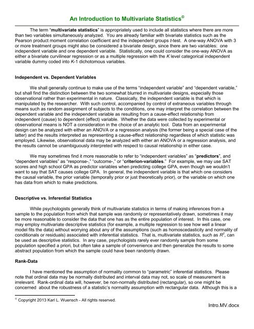
example of SEM including latent variables, consider the research by Greenwald and Gillmore (Journal of
Educational Psychology, 1997, 89, 743-751) on the validity of student ratings of instruction (check out my
review of this research). Their analysis indicated that when students expect to get better grades in a class they
work less on that class and evaluate the course and the instructor more favorably. The indicators (measured
variables) for the Workload latent variable were questions about how much time the students spent on the
course and how challenging it was. Relative expected grade (comparing the grade expected in the rated
course with that the student usually got in other courses) was a more important indicator of the Expected
Grade latent variable than was absolute expected grade. The Evaluation latent variable was indicated by
questions about challenge, whether or not the student would take this course with the same instructor if e had
it to do all over again, and assorted items about desirable characteristics of the instructor and course.
Greenwald’s research suggests that instructors who have lenient grading policies will get good
evaluations but will not motivate their students to work hard enough to learn as much as they do with
instructors whose less lenient grading policies lead to more work but less favorable evaluations.
I am rather skeptical with respect to SEM. Part of my reluctance to embrace SEM stems from my not
being comfortable with the notion that showing good fit between an observed correlation matrix and one’s
theoretical model really “confirms” that model. It is always quite possible that an untested model would fit the
data as well or better than the tested model.

10
Workload
.57
Hours Worked per
Credit Hour
Relative
Expected
Grade
.98
–.49 .75
Expected
Grade
Intellectual Challenge
Absolute
Expected
Grade
.70
.44 .53
Take Same Instructor Again
Evaluation
.93
.90
Characteristics of Instructor & Course
Confirmatory factor analysis can be considered a special case of SEM. In confirmatory factor
analysis the focus is on testing an a priori model of the factor structure of a group of measured variables.
Tabachnick and Fidell (5 th edition) present an example (pages 732 - 749) in which the tested model
hypothesizes that intelligence in learning disabled children, as estimated by the WISC, can be represented by
two factors (possibly correlated with one another) with a particular simple structure (relationship between the
indicator variables and the factors).
DISCRIMINANT FUNCTION ANALYSIS
You wish to predict group membership from a set of two or more continuous variables. The analysis
creates a set of discriminant functions (weighted combinations of the predictors) that will enable you to
predict into which group a case falls, based on scores on the predictor variables (usually continuous, but
could include dichotomous variables and dummy coded categorical predictors). The total possible number of
discriminant functions is one less than the number of groups, or the number of predictor variables, whichever is
less. Generally only a few of the functions will do a good job of discriminating group membership. The second
function, orthogonal to the first, analyses variance not already captured by the first, the third uses the residuals
from the first and second, etc. One may think of the resulting functions as dimensions on which the groups
differ, but one must remember that the weights are chosen to maximize the discrimination among groups,
not to make sense to you. Standardized discriminant function coefficients (weights) and loadings
(correlations between discriminant functions and predictor variables) may be used to label the functions. One
might also determine how well a function separates each group from all the rest to help label the function. It is
possible to do hierarchical/stepwise analysis and factorial (more than one grouping variable) analysis.
Consider what the IRS does with the data they collect from “random audits” of taxpayers. From each
taxpayer they collect data on a number of predictor variables (gross income, number of exemptions, amount of
deductions, age, occupation, etc.) and one classification variable, is the taxpayer a cheater (underpaid e’s
taxes) or honest. From these data they develop a discriminant function model to predict whether or not a

11
return is likely fraudulent. Next year their computers automatically test every return, and if yours fits the
profile of a cheater you are called up for a “discriminant analysis” audit. Of course, the details of the model are
a closely guarded secret, since if a cheater knew the discriminant function e could prepare his return with the
maximum amount of cheating that would result in e’s (barely) not being classified as a cheater.
As another example, consider the research done by Poulson, Braithwaite, Brondino, and Wuensch
(1997, Journal of Social Behavior and Personality, 12, 743-758). Subjects watched a simulated trial in which
the defendant was accused of murder and was pleading insanity. There was so little doubt about his having
killed the victim that none of the jurors voted for a verdict of not guilty. Aside from not guilty, their verdict
options were Guilty, NGRI (not guilty by reason of insanity), and GBMI (guilty but mentally ill). Each mock juror
filled out a questionnaire, answering 21 questions (from which 8 predictor variables were constructed) about
e’s attitudes about crime control, the insanity defense, the death penalty, the attorneys, and e’s assessment of
the expert testimony, the defendant’s mental status, and the possibility that the defendant could be
rehabilitated. To avoid problems associated with multicollinearity among the 8 predictor variables (they were
very highly correlated with one another, and such multicollinearity can cause problems in a multivariate
analysis), the scores on the 8 predictor variables were subjected to a principal components analysis, with the
resulting orthogonal components used as predictors in a discriminant analysis. The verdict choice (Guilty,
NGRI, or GBMI) was the criterion variable.
Both of the discriminant functions were significant. The first function discriminated between jurors
choosing a guilty verdict and subjects choosing a NGRI verdict. Believing that the defendant was mentally ill,
believing the defense’s expert testimony more than the prosecution’s, being receptive to the insanity defense,
opposing the death penalty, believing that the defendant could be rehabilitated, and favoring lenient treatment
were associated with rendering a NGRI verdict. Conversely, the opposite orientation on these factors was
associated with rendering a guilty verdict. The second function separated those who rendered a GBMI verdict
from those choosing Guilty or NGRI. Distrusting the attorneys (especially the prosecution attorney), thinking
rehabilitation likely, opposing lenient treatment, not being receptive to the insanity defense, and favoring the
death penalty were associated with rendering a GBMI verdict rather than a guilty or NGRI verdict.
MULTIPLE ANALYSIS OF VARIANCE, MANOVA
This is essentially a DFA turned around. You have two or more continuous Y’s and one or more
categorical X’s. You may also throw in some continuous X’s (covariates, giving you a MANCOVA, multiple
analysis of covariance). The most common application of MANOVA in psychology is as a device to guard
against inflation of familywise alpha when there are multiple dependent variables. The logic is the same as
that of the protected t-test, where an omnibus ANOVA on your K-level categorical X must be significant before
you make pairwise comparisons among your K groups’ means on Y. You do a MANOVA on your multiple Y’s.
If it is significant, you may go on and do univariate ANOVAs (one on each Y), if not, you stop. In a factorial
analysis, you may follow-up any effect which is significant in the MANOVA by doing univariate analyses for
each such effect.
As an example, consider the MANOVA I did with data from a simulated jury trial with Taiwanese
subjects (see Wuensch, Chia, Castellow, Chuang, & Cheng, Journal of Cross-Cultural Psychology, 1993, 24,
414-427). The same experiment had earlier been done with American subjects. X’s consisted of whether or
not the defendant was physically attractive, sex of the defendant, type of alleged crime (swindle or burglary),
culture of the defendant (American or Chinese), and sex of subject (juror). Y’s consisted of length of sentence
given the defendant, rated seriousness of the crime, and ratings on 12 attributes of the defendant. I did two
MANOVAs, one with length of sentence and rated seriousness of the crime as Y’s, one with ratings on the 12
attributes as Y’s. On each I first inspected the MANOVA. For each effect (main effect or interaction) that was
significant on the MANOVA, I inspected the univariate analyses to determine which Y’s were significantly
associated with that effect. For those that were significant, I conducted follow-up analyses such as simple
interaction analyses and simple main effects analyses. A brief summary of the results follows: Female
subjects gave longer sentences for the crime of burglary, but only when the defendant was American;
attractiveness was associated with lenient sentencing for American burglars but with stringent sentencing for
American swindlers (perhaps subjects thought that physically attractive swindlers had used their attractiveness

12
in the commission of the crime and thus were especially deserving of punishment); female jurors gave more
lenient sentences to female defendants than to male defendants; American defendants were rated more
favorably (exciting, happy, intelligent, sociable, strong) than were Chinese defendants; physically attractive
defendants were rated more favorably (attractive, calm, exciting, happy, intelligent, warm) than were physically
unattractive defendants; and the swindler was rated more favorably (attractive, calm, exciting, independent,
intelligent, sociable, warm) than the burglar.
In MANOVA the Y’s are weighted to maximize the correlation between their linear combination and the
X’s. A different linear combination (canonical variate) is formed for each effect (main effect or interaction—in
fact, a different linear combination is formed for each treatment df—thus, if an independent variable consists
of four groups, three df, there are three different linear combinations constructed to represent that effect, each
orthogonal to the others). Standardized discriminant function coefficients (weights for predicting X from
the Y’s) and loadings (for each linear combination of Y’s, the correlations between the linear combination and
the Y’s themselves) may be used better to define the effects of the factors and their interactions. One may
also do a “stepdown analysis” where one enters the Y’s in an a priori order of importance (or based solely on
statistical criteria, as in stepwise multiple regression). At each step one evaluates the contribution of the newly
added Y, above and beyond that of the Y’s already entered.
As an example of an analysis which uses more of the multivariate output than was used with the
example two paragraphs above, consider again the research done by Moore, Wuensch, Hedges, and
Castellow (1994, discussed earlier under the topic of log-linear analysis). Recall that we manipulated the
physical attractiveness and social desirability of the litigants in a civil case involving sexual harassment. In
each of the experiments in that study we had subjects fill out a rating scale, describing the litigant (defendant or
plaintiff) whose attributes we had manipulated. This analysis was essentially a manipulation check, to verify
that our manipulations were effective. The rating scales were nine-point scales, for example,
Awkward
Poised
1 2 3 4 5 6 7 8 9
There were 19 attributes measured for each litigant. The data from the 19 variables were used as
dependent variables in a three-way MANOVA (social desirability manipulation, physical attractiveness
manipulation, gender of subject). In the first experiment, in which the physical attractiveness and social
desirability of the defendant were manipulated, the MANOVA produced significant effects for the social
desirability manipulation and the physical attractiveness manipulation, but no other significant effects. The
canonical variate maximizing the effect of the social desirability manipulation loaded most heavily (r > .45) on
the ratings of sociability (r = .68), intelligence (r = .66), warmth (r = .61), sensitivity (r = .50), and kindness (r =
.49). Univariate analyses indicated that compared to the socially undesirable defendant, the socially desirable
defendant was rated significantly more poised, modest, strong, interesting, sociable, independent, warm,
genuine, kind, exciting, sexually warm, secure, sensitive, calm, intelligent, sophisticated, and happy. Clearly
the social desirability manipulation was effective.
The canonical variate that maximized the effect of the physical attractiveness manipulation loaded
heavily only on the physical attractiveness ratings (r = .95), all the other loadings being less than .35. The
mean physical attractiveness ratings were 7.12 for the physically attractive defendant and 2.25 for the
physically unattractive defendant. Clearly the physical attractiveness manipulation was effective. Univariate
analyses indicated that this manipulation had significant effects on several of the ratings variables. Compared
to the physically unattractive defendant, the physically attractive defendant was rated significantly more poised,
strong, interesting, sociable, physically attractive, warm, exciting, sexually warm, secure, sophisticated, and
happy.
In the second experiment, in which the physical attractiveness and social desirability of the plaintiff
were manipulated, similar results were obtained. The canonical variate maximizing the effect of the social
desirability manipulation loaded most heavily (r > .45) on the ratings of intelligence (r = .73), poise (r = .68),
sensitivity (r = .63), kindness (r = .62), genuineness (r = .56), warmth (r = .54), and sociability (r = .53).
Univariate analyses indicated that compared to the socially undesirable plaintiff the socially desirable plaintiff
was rated significantly more favorably on all nineteen of the adjective scale ratings.

The canonical variate that maximized the effect of the physical attractiveness manipulation loaded
heavily only on the physical attractiveness ratings (r = .84), all the other loadings being less than .40. The
mean physical attractiveness ratings were 7.52 for the physically attractive plaintiff and 3.16 for the physically
unattractive plaintiff. Univariate analyses indicated that this manipulation had significant effects on several of
the ratings variables. Compared to the physically unattractive plaintiff the physically attractive plaintiff was
rated significantly more poised, interesting, sociable, physically attractive, warm, exciting, sexually warm,
secure, sophisticated, and happy.
13
LEAST SQUARES ANOVA
An ANOVA may be done as a multiple regression, with the categorical X’s coded as “dummy variables.”
A K-level X is represented by K-1 dichotomous dummy variables. An interaction between two X’s is
represented by products of the main effects X’s. For example, were factors A and B both dichotomous, we
could code A with X 1 (0 or 1), B with X 2 (0 or 1), and A x B with X 3 , where X 3 equals X 1 times X 2 . Were A
dichotomous and B had three levels, the main effect of B would require two dummy variables, X 2 and X 3 , and
the A x B interaction would require two more dummy variables, X 4 (the product of X 1 and X 2 ) and X 5 (the
product of X 1 and X 3 ). [Each effect will require as many dummy variables as the df it has.] In the multiple
regression the SS due to X 1 would be the SS A , the SS B would be the combined SS for X 2 and X 3 , and the
interaction SS would be the combined SS for X 4 and X 5 . There are various ways we can partition the SS, but
we shall generally want to use Overall and Spiegel’s Method I, where each effect is partialled for all other
effects. That is, for example, SS A is the SS that is due solely to A (the increase in the SS reg when we added
A’s dummy variable(s) to a model that already includes all other effects). Any variance in Y that is ambiguous
(could be assigned to more than one effect) is disregarded. There will, of course, be such ambiguous variance
only when the independent variables are nonorthogonal (correlated, as indicated by the unequal cell sizes).
Overall and Spiegel’s Method I least-squares ANOVA is the method that is approximated by the “by hand”
unweighted means ANOVA that you learned earlier.
ANCOV
In the analysis of covariance you enter one or more covariates (usually continuous, but may be
dummy coded categorical variables) into the multiple correlation before or at the same time that you enter
categorical predictor variables (dummy codes). The effect of each factor or interaction is the increase in the
SS reg when that factor is added to a model that already contains all of the other factors and interactions and all
of the covariates.
In the ideal circumstance, you have experimentally manipulated the categorical variables (independent
variables), randomly assigned subjects to treatments, and measured the covariate(s) prior to the manipulation
of the independent variable. In this case, the inclusion of the covariate(s) in the model will reduce what would
otherwise be error in the model, and this can greatly increase the power of your analysis. Consider the
following partitioning of the sums of squares of post-treatment wellness scores. The Treatment variable is
Type of Therapy used with your patients, three groups. The F ratio testing the treatment will be the ratio of the
Treatment Mean Square to the Error Mean Square.
Sums of Squares
Treatment
Error

14
Your chances of getting a significant result are going to be a lot better if you can do something to
reduce the size of the error variance, which goes into the denominator of the F ratio. Reducing the size of the
Mean Square Error (the denominator of the F ratio) will increase the value of F and lower the p value.
Suppose you find that you have, for each of your subjects, a score on the wellness measure taken prior to the
treatment. Those baseline scores are likely well correlated with the post-treatment scores. You add the
baseline wellness to the model. – that is, baseline wellness becomes a covariate.
Sum of Squares
Treatment
Baseline
Error
Wow! You have cut the error in half. This will greatly increase the value of the F testing the effect of
the treatment. In statistics, getting a big F is generally a good thing, as it leads to significant results.
Now you discover that you also have, for each subject, a pre-treatment measure of blood levels of
scatophobin, a neurohormone thought to be associated with severity of the treated illness. You now include
that as a second covariate.
Sum of Squares
Treatment
Baseline
Scatophobin
Error
Double WOW! You have reduced the error variance even more, gaining additional power and
additional precision with respect to your estimates of effect sizes (tighter confidence intervals).
If your categorical predictor variables are correlated with the covariate(s), then removing the
effects of the covariates may also remove some of the effects of the factors, which may not be what you
wanted to do. Such a confounding of covariates with categorical predictors often results from:
subjects not being randomly assigned to treatments
the covariates being measured after the manipulations of the independent variables(s) -- and those
manipulations changed subjects’ scores on the covariates
the categorical predictors being nonexperimental (not manipulated),
Typically the psychologist considers the continuous covariates to be nuisance variables, whose effects
are to be removed prior to considering the effects of categorical predictor variables. The same model can be
used to predict scores on a continuous outcome variable from a mixture of continuous and categorical
predictor variables, even when the researcher does not consider the continuous covariates to be nuisance
variables. For example, consider the study by Wuensch and Poteat discussed earlier as an example of logistic
regression. A second dependent variable was respondents’ scores on a justification variable (after reading the
case materials, each participant was asked to rate on a 9-point scale how justified the research was, from “not
at all” to “completely”). We used an ANCOV model to predict justification scores from idealism, relativism,
gender, and scenario. Although the first two predictors were continuous (“covariates”), we did not consider

them to be nuisance variables, we had a genuine interest in their relationship with the dependent variable.
A brief description of the results of the ANCOV follows:
15
There were no significant interactions between predictors, but each predictor had a significant main
effect. Idealism was negatively associated with justification, = 0.32, r = 0.36, F(1, 303) = 40.93, p < .001,
relativism was positively associated with justification, = .20, r = .22, F(1, 303) = 15.39, p < .001, mean
justification was higher for men (M = 5.30, SD = 2.25) than for women (M = 4.28, SD = 2.21), F(1, 303) =
13.24, p < .001, and scenario had a significant omnibus effect, F(4, 303) = 3.61, p = .007. Using the medical
scenario as the reference group, the cosmetic and the theory scenarios were found to be significantly less
justified.
MULTIVARIATE APPROACH TO REPEATED MEASURES ANOVA
An ANOVA may include one or more categorical predictors for which the groups are not independent.
Subjects may be measured at each level of the treatment variable (repeated measures, within-subjects).
Alternatively, subjects may be blocked on the basis of variables known to be related to the dependent variable
and then, within each block, randomly assigned to treatments (the randomized blocks or split-plot design). In
either case, a repeated measures ANOVA may be appropriate if the dependent variable is normally distributed
and other assumptions are met.
The traditional repeated measures analyses of variance (aka “univariate approach”) has a sphericity
assumption: the standard error of the difference between pairs of means is constant across all pairs of
means. That is, for comparing the mean at any one level of the repeated factor versus any other level of the
repeated factor, the diff is the same as it would be for any other pair of levels of the repeated factor. Howell
(page 443 of the 6 th edition of Statistical Methods for Psychology) discusses compound symmetry, a
somewhat more restrictive assumption. There are adjustments (of degrees of freedom) to correct for violation
of the sphericity assumption, but at a cost of lower power.
A more modern approach, the multivariate approach to repeated measures designs, does not have
such a sphericity assumption. In the multivariate approach the effect of a repeated measures dimension (for
example, whether this score represents Suzie Cue’s headache duration during the first, second, or third week
of treatment) is coded by computing k1 difference scores (one for each degree of freedom for the repeated
factor) and then treating those difference scores as dependent variables in a MANOVA.
You are already familiar with the basic concepts of main effects, interactions, and simple effects from
our study of independent samples ANOVA. We remain interested in these same sorts of effects in ANOVA
with repeated measures, but we must do the analysis differently. While it might be reasonable to conduct such
an analysis by hand when the design is quite simple, typically computer analysis will be employed.
If your ANOVA design has one or more repeated factors and multiple dependent variables, then you
can do a doubly multivariate analysis, with the effect of the repeated factor being represented by a set of
k1 difference scores for each of the two or more dependent variables. For example, consider my study on the
effects of cross-species rearing of house mice (Animal Learning & Behavior, 1992, 20, 253-258). Subjects
were house mice that had been reared by house mice, deer mice, or Norway rats. The species of the foster
mother was a between-subjects (independent samples) factor. I tested them in an apparatus where they could
visit four tunnels: One scented with clean pine shavings, one scented with the smell of house mice, one
scented with the smell of deer mice, and one scented with the smell of rats. The scent of the tunnel was a
within-subjects factor, so I had a mixed factorial design (one or more between-subjects factor, one or more
within-subjects factor). I had three dependent variables: The latency until the subject first entered each tunnel,
how many visits the subject made to each tunnel, and how much time each subject spent in each tunnel.
Since the doubly multivariate analysis indicated significant effects (interaction between species of the foster
mother and scent of the tunnel, as well as significant main effects of each factor), singly multivariate ANOVA
(that is, on one dependent variable at a time, but using the multivariate approach to code the repeated factor)
was conducted on each dependent variable (latency, visits, and time). The interaction was significant for each

16
dependent variable, so simple main effects analyses were conducted. The basic finding (somewhat
simplified here) was that with respect to the rat-scented tunnel, those subjects who had been reared by a rat
had shorter latencies to visit the tunnel, visited that tunnel more often, and spent more time in that tunnel. If
you consider that rats will eat house mice, it makes good sense for a house mouse to be disposed not to enter
tunnels that smell like rats. Of course, my rat-reared mice may have learned to associate the smell of rat with
obtaining food (nursing from their rat foster mother) rather than being food!
CLUSTER ANALYSIS
In a cluster analysis the goal is to cluster cases (research units) into groups that share similar
characteristics. Contrast this goal with the goal of principal components and factor analysis, where one groups
variables into components or factors based on their having similar relationships with with latent variables.
While cluster analysis can also be used to group variables rather than cases, I have no familiarity with that
application.
I have never had a set of research data for which I though cluster analysis appropriate, but I wanted to
play around with it, so I obtained, from online sources, data on faculty in my department: Salaries, academic
rank, course load, experience, and number of published articles. I instructed SPSS to group the cases (faculty
members) based on those variables. I asked SPSS to standardize all of the variables to z scores. This
results in each variable being measured on the same scale and the variables being equally weighted. I had
SPSS use agglomerative hierarchical clustering. With this procedure each case initially is a cluster of its
own. SPSS compares the distance between each case and the next and then clusters together the two cases
which are closest. I had SPSS use the squared Euclidian distance between cases as the measure of
v
distance. This is quite simply 2
X
i
Y i
i 1
, the sum across variables (from i = 1 to v) of the squared
difference between the score on variable i for the one case (X i ) and the score on variable i for the other case
(Y i ). At the next step SPSS recomputes all the distances between entities (cases and clusters) and then
groups together the two with the smallest distance. When one or both of the entities is a cluster, SPSS
computes the averaged squared Euclidian distance between members of the one entity and members of the
other entity. This continues until all cases have been grouped into one giant cluster. It is up to the researcher
to decide when to stop this procedure and accept a solution with k clusters. K can be any number from 1 to
the number of cases.
SPSS produces both tables and graphics that help the analyst follow the process and decide which
solution to accept I obtained 2, 3, and 4 cluster solutions. In the k = 2 solution the one cluster consisted of all
the adjunct faculty (excepting one) and the second cluster consisted of everybody else. I compared the two
clusters (using t tests) and found compared to the regular faculty the adjuncts had significantly lower salary,
experience, course load, rank, and number of publications.
In the k = 3 solution the group of regular faculty was split into two groups, with one group consisting of
senior faculty (those who have been in the profession long enough to get a decent salary and lots of
publications) and the other group consisting of junior faculty (and a few older faculty who just never did the
things that gets one merit pay increases). I used plots of means to show that the senior faculty had greater
salary, experience, rank, and number of publications than did the junior faculty.
In the k = 4 solution the group of senior faculty was split into two clusters. One cluster consisted of the
acting chair of the department (who had a salary and a number of publications considerably higher than the
others) and the other cluster consisting of the remaining senior faculty (excepting those few who had been
clustered with the junior faculty).
There are other ways of measuring the distance between clusters and other methods of doing the
clustering. For example, one can do divisive hierarchical clustering, in which one starts out with all cases in
one big cluster and then splits off cases into new clusters until every case is a cluster all by itself.

17
Aziz and Zickar (2006: A cluster analysis investigation of workaholism as a syndrome, Journal of
Occupational Health Psychology, 11, 52-62) is a good example of the use of cluster analysis with
psychological data. Some have defined workaholism as being high in work involvement, high in drive to work,
and low in work enjoyment. Aziz and Zickar obtained measures of work involvement, drive to work, and work
enjoyment and conducted a cluster analysis. One of the clusters in the three-cluster solution did look like
workaholics – high in work involvement and drive to work but low in work enjoyment. A second cluster
consisted of positively engaged workers (high on work involvement and work enjoyment) and a third consisted
of unengaged workers (low in involvement, drive, and enjoyment).
Multivariate Effect Size Estimation – supplemental chapter from Kline, Rex. B. (2004).
Beyond significance testing: Reforming data analysis methods in behavioral research.
Washington, DC: American Psychological Association.
Statistics Lessons
MANOVA, Familywise Error, and the Boogey Man
SAS Lessons
SPSS Lessons
Endnote
† A high Scale 5 score indicates that the individual is more like members of the other gender than are most
people. A man with a high Scale 5 score lacks stereotypical masculine interests, and a woman with a high
Scale 5 score has interests that are stereotypically masculine. Low Scale 5 scores indicate stereotypical
masculinity in men and stereotypical femininity in women. MMPI Scale scores are “T-scores” – that is, they
have been standardized to mean 50, standard deviation 10. The normative group was residents of Minnesota
in the 1930’s. The MMPI-2 was normed on what should be a group more representative of US residents.
Copyright 2013 Karl L. Wuensch - All rights reserved.