The frequency structure matrix: A representation of color filter arrays

The Frequency Structure Matrix: A Representation of
Color Filter Arrays
Yan Li, 1 Pengwei Hao, 2,3 Zhouchen Lin 4
1 Pattern Recognition Laboratory, Delft University of Technology, 2628 CD Delft, The Netherlands
2 Department of Computer Science, Queen Mary, University of London, London E1 4NS, UK
3 Center for Information Science, Peking University, Beijing 100871, China
4 Microsoft Research Asia, Beijing 100190, China
Received 11 February 2009; accepted 24 May 2010
ABSTRACT: This article introduces the frequency structure matrix as
a new representation of color filter arrays (CFAs). The matrix records
the frequency components of CFA filtered images and their positions
in the spectrum. The matrix can be conveniently obtained by applying
the symbolic DFT to the CFA pattern. With this new representation, it
is easy to analyze the characteristics of CFAs and to formulate the
CFA design as an optimization problem. VC 2011 Wiley Periodicals, Inc.
Int J Imaging Syst Technol, 21, 101–106, 2011; Published online in Wiley Online
Library (wileyonlinelibrary.com). DOI 10.1002/ima.20252
Key words: color filter array (CFA); discrete Fourier transform (DFT);
sampling; multiplexing; demosaicking
I. INTRODUCTION
To reduce cost, size, and complexity, color filter arrays (CFAs)
are commonly used in consumer digital cameras. A CFA is a
mosaic of optically selective filters, each filtering the incident
light projected to one pixel. Therefore, the sensed image has only
one color at each pixel. The missing two colors of each pixel
have to be estimated by methods called demosaicking. The most
widely used CFA was the Bayer CFA (Bayer, 1976) [Fig. 1(a)],
whose sampling rates for green, red and blue (G, R, and B) are
1/2, 1/4, and 1/4, respectively.
The representation of CFA is crucial. Different representations
lead to different demosaicking algorithms. For the CFA design, an
appropriate representation is also necessary as it requires proper mathematical
modeling for optimization. The spatial representation could
not provide enough insight into why a demosaicking algorithm can
work well, hence is inadequate for the CFA design. Since the spectral
representation can reveal the structure and composition of frequencies,
it is more suitable for theoretical analysis on the performance of CFAs
and the corresponding demosaicking algorithms.
Correspondence to: Yan Li; e-mail: yan.li@tudelft.nl
There has been some prior work on analyzing the spectral components
of CFA filtered images (Alleysson et al., 2005; Dubois, 2005; Hirakawa
and Wolfe, 2007; Dubois, 2008; Hirakawa and Wolfe, 2008).
Alleysson et al. (2005) and Dubois (2005) showed that in the frequency
domain, a Bayer CFA filtered image has one luminance component at
the baseband and several chrominance ones modulated at higher frequencies
(Fig. 1(b)). An image sampled with any CFA was represented
with a green component and those that correspond to differences
between colors (Hirakawa and Wolfe, 2007; Hirakawa and Wolfe,
2008). To design a CFA, one can first specify the modulation points of
frequency components and then select a set of parameters satisfying
some constraints. A CFA filtered image was represented as a sum of different
combinations of the original components, which correspond to
components modulated at different frequencies (Dubois, 2008). This
combination was represented using several matrices, which record parameters
of the components in the frequency domain. Based on this representation,
a demosaicking method by demultiplexing the frequency
components was also proposed in that paper.
However, the existing representations have some limitations.
For example, they are not very intuitive, not revealing enough of
the relationship between a CFA and its spectral representation and a
bit too complex to calculate. So when applied to the CFA design,
these representations often cause some difficulties. For example,
one cannot easily express a CFA and its spectral representation
with the same set of parameters. Thus, it is difficult to design CFAs
using a unified framework, by expressing all the constraints and the
objective function mathematically.
In this article, we propose a new representation, the frequency
structure matrix, which records the frequency components at all the
modulation points. It is more intuitive and informative, and directly
related to the CFA. The matrix can be easily obtained by computing
the symbolic DFT of the CFA pattern. With this representation, the
CFA design can be formulated as an optimization problem (Li et al,
2008b).
' 2011 Wiley Periodicals, Inc.

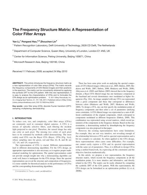
Figure 1. Bayer CFA pattern (Bayes, 1976) and the spectrum of the ‘window’ image filtered with it. (c)–(f) show each component in the spectrum
(b). (c) (F (R) 1 2F (G) 1 F (B) )/4 at frequency point (0,0), (d) (2F (R) 1 F (B) )/4 modulated at (0.5,0), (e) (F (R) 2F (B) )/4 at (0,0.5), and (f) (2F (R) 1 2F (G)
2F (B) )/4 at (0.5,0.5). The ‘window’ is a commonly used test image from the Kodak dataset (Alleysson et al., 2005). [Color figure can be viewed in
the online issue, which is available at wileyonlinelibrary.com.]
II. THE FREQUENCY STRUCTURE MATRIX
Figure 1b shows the spectrum of the image ‘‘window’’ filtered with
the Bayer CFA. As shown by Alleysson et al., (2005) and Dubois,
(2005), it contains several frequency components: (F (R) 1 2F (G) 1
F (B) )/4 at frequency point (0,0), (2F (R) 1 F (B) )/4 modulated at (0.5,
0), (F (R) 2 F (B) )/4 at (0,0.5), and (2F (R) 1 2F (G) 2 F (B) )/4 at (0.5,
0.5), where F (R) , F (G) , and F (B) denote the DFT spectra of the original
image of primary colors R, G, and B, respectively, and one period
in the frequency domain is a square [0,1) 2 . It is also shown that
images filtered with any CFA have similar spectra, consisting of
several components modulated at different frequency points (Hirakawa
and Wolfe, 2007; Dubois, 2008; Hirakawa and Wolfe, 2008).
Inspired by the observed patterns of the spectra of CFA filtered
images, we propose to represent the spectra by faithfully recording the
frequency components: their frequency details and their positions.
Such information can naturally be arranged in a matrix form. Therefore,
we call it the frequency structure matrix. For example, we may
represent the spectrum of an image filtered with the Bayer CFA as:
S Bayer ¼ 1
F ðRÞ þ 2F ðGÞ þ F ðBÞ F ðRÞ þ F ðBÞ
4 F ðRÞ F ðBÞ F ðRÞ þ 2F ðGÞ F ðBÞ
:
(Note that by convention the spectra of images are displayed with
(0,0) being at the center, while in the frequency structure matrix,
(0,0) is at the top-left corner of the matrix. The readers should circularly
shift either of them in order to match them.) One can see
that all the information of the spectra that is of interest to him/her
can be found in S Bayer .
In the following, we present the formal definition of the frequency
structure matrix. We also prove that the frequency structure
matrix can be easily calculated by applying the symbolic DFT to
the CFA pattern. For brevity, sometimes we may write ‘‘frequency
structure’’ instead of ‘‘frequency structure matrix.’’
III. FROM SPECTRA TO FREQUENCY STRUCTURE
To obtain the frequency-domain representation, a CFA filtered image
is first represented in the spatial domain by decomposing the image
and the CFA pattern into three channels, corresponding to three primary
colors, respectively. Then, the DFT of the CFA filtered image is
computed using the convolution theory. Once the expression of the
spectrum is available, we can identify its frequency components and
their corresponding positions in the frequency domain. Then, we can
arrange these components into a matrix form, according to their positions,
and obtain the frequency structure matrix.
102 Vol. 21, 101–106 (2011)

Figure 2. The Bean CFA pattern (Bean, 2003) and the spectra of the ‘window’ image filtered with it. (a) The Bean CFA pattern, (b) the spectrum
F (B)
Bean of the blue channel of the Bean CFA filtered image, represented by the frequency structure (8), (c) the spectrum F Bean of the Bean CFA filtered
image, represented by the frequency structure (11) or (13). [Color figure can be viewed in the online issue, which is available at
wileyonlinelibrary.com.]
A. Spectra of CFA Filtered Images. A CFA h CFA (x,y) is usually
a periodic tiling of a much smaller array called the CFA pattern
h p (x,y). Using the well-established tri-primary color theory, a CFA
pattern can be decomposed into three primary CFA patterns
h ðCÞ
p
ðx; yÞ, each accounting for one primary color C (Alleysson et al.,
2005; Hirakawa and Wolfe, 2007; Dubois, 2008). Then, symbolically
we can write:
h p ¼ X C
h ðCÞ
p C: ð1Þ
To ensure the same dynamic range of the sensed image at all pixels,
the sum of all primary CFA patterns should be an all-one matrix
X
h ðCÞ
p ðx; yÞ ¼1; 8x; y: ð2Þ
C
For example, for the Bean CFA pattern h Bean 5 [C M;BY] (Fig. 2a),
the primary CFA patterns of colors R, G, and B are respectively:
2
0 1 3 2
1
3
Bean ¼ 6 2 7
4
0 1 5; h ðGÞ
Bean ¼ 6 2 0 7
4
0 1 2
2
h ðRÞ
5;h ðBÞ
2
1
3
1
Bean ¼ 4 2 2 5;
1 0
as M 5 (R 1 B)/2, Y 5 (R 1 G)/2 and C 5 (G 1 B)/2.
Let f(x,y) be the full color image of size (N x ,N y ) and the CFA
pattern h p (x,y) be of size (n x ,n y ). Then, the CFA filtered image is:
f CFA ðx; yÞ ¼ X C
f ðCÞ ðx; yÞh ðCÞ
CFAðx; yÞ; ð4Þ
where f ðCÞ ðx; yÞ is the color C component of f and h ðCÞ
CFAðx; yÞ is the
corresponding CFA of color C defined as the periodic replica of the
primary CFA pattern h ðCÞ
p ðx; yÞ:
h ðCÞ
CFAðx; yÞ ¼hðCÞ p ðx mod n x; y mod n y Þ:
H
Without loss of generality, we assume that N x and N y are multiples
of n x and n y , respectively. We first compute the spectrum of
ðx; yÞ (Li et al., 2008):
h ðCÞ
CFA
ðCÞ
CFA ðx x; x y Þ¼DFT½h ðCÞ
CFAðx; yÞŠ
where H ðCÞ
p
¼ 1
Nx X 1
N x N y x¼0
(
¼
XN y 1
y¼0
h ðCÞ
i2pðxxxþyxyÞ
CFAðx; yÞe
HðCÞ p ðx x ; x y Þ; if n x x x 2 Z and n y x y 2 Z;
0; otherwise;
ðx x ; x y Þ is the DFT of the primary CFA pattern
h ðCÞ
p ðx; yÞ. Note that here (x x ,x y ) takes discrete values in the square
[0,1) 2 (at a stepsize of (1/N x ,1/N y ) for H ðCÞ
CFA and (1/n x,1/n y ) for Hp ðCÞ ,
respectively) instead of discrete indices of the signals because we have
found that it is more convenient to normalize the frequencies. The above
equality shows that the spectrum of a CFA is a sampling of the spectrum
of its CFA pattern at frequencies (k x /n x ,k y /n y ), where (k x ,k y ) [ Z 2 .
As multiplication in the spatial domain corresponds to the circular
convolution in the frequency domain, the DFT of f ðCÞ
CFA can be
found to be (Li et al., 2008):
F ðCÞ
CFA ðx x; x y Þ¼DFT½f ðCÞ ðx; yÞh ðCÞ
CFA
¼ Xnx 1 Xn y 1
k x¼0 k y¼0
H ðCÞ
p
k x
n x
; k y
n y
ðx; yÞŠ
F ðCÞ k x
x x ; x y
n x
k y
n y
ð5Þ
: ð6Þ
where F ðCÞ k
x x k
x n x
; x
y
y n y
has been circularly shifted. This
implies that in the frequency domain the spectrum F ðCÞ
CFA
is a multiplexing
of n x n y frequency components centered at (k x /n x ,k y /n y ),k x 5
0,1,...,n x 2 1;k y 5 0,1,...,n y 2 1, and each component is the original
spectrum F ðCÞ weighted by Hp
ðCÞ ðk x =n x ; k y =n y Þ, the spectral value of
the CFA pattern at the corresponding frequency. Figure 2b shows
an example of the spectrum.
B. The Frequency Structure. As exemplified in Section II and
shown by Li et al. (2008), it will be more intuitive and useful to
arrange the identified frequency components in a matrix form.
Therefore, we use a matrix S ðCÞ
CFA
Eq. (6):
to represent the spectrum FðCÞ CFA in
Vol. 21, 101–106 (2011) 103

Figure 3. Some existing CFA patterns. The second row are the spectra of image ‘window’ sampled with the corresponding CFAs in the first
row. (a) Yamanaka (1977), (b) Diagonal Stripe (Lukac and Plataniotis, 2005), (c) Dillon (1977). [Color figure can be viewed in the online issue, which
is available at wileyonlinelibrary.com.]
S ðCÞ
CFA ¼
HðCÞ p
k x
; k
y
n x n y
F ðCÞ ðxÞ
kx ¼ 0; 1; :::; nx 1;
ky ¼ 0; 1; :::; ny 1: ð7Þ
The entries of the matrix S CFA are actually:
S CFA ðk x ; k y Þ¼ X C
H ðCÞ
p
k x
; k
y
n x n y
F ðCÞ ðx x ; x y Þ;
ð10Þ
It records all the information about the frequency components of
F ðCÞ
CFA : the (k x, k y )-th entry S ðCÞ
CFA ðk x; k y Þ is the frequency component
centered at (k x /n x , k y /n y ). We call this matrix the frequency structure
of the primary CFA h ðCÞ
CFA
of color C.
For example, for the primary Bean CFA pattern of color blue
(B)
[Eq. (3)], its DFT is DFT[h Bean ] 5 [1/2 1/4; 0 2 1/4] and thus its
frequency structure is
2
3
1 1
S ðBÞ
Bean ¼ 6 2 FðBÞ 4 FðBÞ 7
4
1
5; ð8Þ
0
4 FðBÞ
where F (B) (B)
denotes the spectrum of the blue channel of f. S Bean
(B)
shows that F Bean has three nonzero spectra: one is F (B) /2, at the
baseband, one is F (B) /4, modulated at frequency (1/2, 0) and another
is 2F (B) (B)
/4, at (1/2, 1/2). Figure 2b shows the spectrum F Bean .
Now we are equipped to define the frequency structure matrix of
a CFA pattern. According to (4), we may define the frequency
structure of a CFA pattern as the following matrix:
S CFA ¼ P C
S ðCÞ
CFA :
ð9Þ
k x 5 0, 1,...,n x 2 1; k y 5 0, 1,..., n y 21. The entry S CFA (k x , k y )
denotes the frequency component of the spectrum F CFA centered
(or modulated) at frequency (k x /n x , k y /n y ). Thus the spectrum of
F CFA is a multiplexing of n x . n y components S CFA (k x , k y ) centered
at grid points (k x /n x , k y /n y )(k x 5 0, 1,...,n x 2 1; k y 5 0,1,...,n y 2 1).
For this reason, we refer to the entries (10) in S CFA as the multiplex
components, which are sums of the spectra F ðCÞ weighted by Hp ðCÞ .
For example, the frequency structure of the Bean CFA pattern,
as the sum of S ðCÞ
Bean ; C¼R; G; B, is:
S Bean ¼
2
3
X 1
S ðCÞ
Bean ¼ 4 4 FðRÞ 1 4 FðRÞ 5
0 0
2
1
3 2
þ
4 FðGÞ 0 1 1
3
6
7
4
5 þ 4 2 FðBÞ 4 FðBÞ
5
1
0
4 FðGÞ 0 1
4 FðBÞ
" #
¼ 1 F ðRÞ þ F ðGÞ þ 2F ðBÞ F ðRÞ þ F ðBÞ
4 0 F ðGÞ F ðBÞ
C¼R;G;B
ð11Þ
104 Vol. 21, 101–106 (2011)

This shows that the spectrum F CFA of the Bean CFA filtered image
has three nonzero multiplex components: (F (R) 1 F (G) 1 2F (B) )/4 at
the baseband, (2F (R) 1 F (B) )/4 at (1/2,0), and (F (G) 2 F (B) )/4 at (1/
2, 1/2). Figure 2c shows the spectrum of the ‘‘window’’ image filtered
by the Bean CFA.
By applying DFT to both sides of Eq. (2), we have that:
X
C
H ðCÞ
p
k x
; k
y
n x n y
¼ dðk x Þdðk y Þ;
ð12Þ
which means that the sums of the coefficients for all multiplex components
(10) are zero, except the one at the baseband (frequency
(0,0)), which is 1. As shown by Alleysson et al. (2005) and Dubois
(2005), we shall call the multiplex component at the baseband the
luminance component (luma) and the others the chrominance components
(chromas).
IV. SYMBOLIC DFT TO COMPUTE THE
FREQUENCY STRUCTURE
By the definition in Eq. (10), it seems a little tedious to compute the
frequency structure as we may have to compute the DFT of all the
primary CFA patterns. However, we have found that there is a simple
way to compute the frequency structure of a CFA. To proceed,
we introduce the symbolic DFT of a sequence of symbols. For a
string s 5 s 0 s 1 ...s N21 , its symbolic DFT is a sequence of order 1
polynomials S 5 S 0 S 1 ...S N21 , where
S k ¼ 1 N
X N 1
l¼0
s l e 2pikl=N :
For the 2D case, the symbolic DFT can be defined in an analogous
way. With this definition, we can claim that:
Theorem 1. Ifwe rewrite ‘‘F ðCÞ ðxÞ’’ as ‘‘C’’, then the frequency
structure S CFA is the symbolic DFT of the CFA pattern h p .
Proof. The symbolic DFT of the CFA pattern h p is H p 5
DFT[h p ], where
H p ðk x ; k y Þ¼ 1
nx X 1 Xn y 1
h p ðx; yÞe 2piðxkx=nxþyky=nyÞ
n x n y
¼ 1 X
n x n y
x¼0 y¼0
C Xnx 1 Xn y 1
h ðCÞ
p
C x¼0 y¼0
ðx; yÞe
2piðxkx=nxþyky=nyÞ
¼ P Hp
ðCÞ ðk x =n x ; k y =n y ÞC:
C
where P C
denotes summation among all primary colors C. Hence,
the claim is true by comparing the above with (10).
n
From this theorem, in the sequel, we also use C to represent the
spectrum of the color channel C of the original image.
Similarly, for the frequency structure of the primary CFA patterns,
we also have S ðCÞ
CFA ¼ DFT½hðCÞ p ŠC.
V. EXAMPLES OF FREQUENCY STRUCTURES
Thanks to Theorem 1, the frequency structures of any CFAs can be
easily computed. For example, the frequency structure of the Bean
CFA (Bean, 2003) can be found to be:
2
G þ B R þ B
3
6
S Bean ¼ DFT
2 2 7
4
5
R þ G
B
2
¼ 1
R þ G þ 2B R þ B
:
4 0 G B
ð13Þ
As proven by Theorem 1, this representation is the same as that of
Eq. (11), if ‘‘F ðCÞ ðxÞ’’ is rewritten as ‘‘C’’.
Now we show more examples. The frequency structures of the CFA
(Yamanaka, 1977), the Diagonal CFA (Lukac and Plataniotis, 2005),
and the Dillon CFA (Dillion, 1977) are, respectively, as follows:
S Yam ¼ DFT G R G B
G B G R
¼ F
L 0 F C1 0
;
0 F C2 0 F C2
where F L 5 (R 1 2G 1 B)/4, F C1 5 (2R 1 2G 2 B)/4 and F C2 5
(2R 1 B)/4;
2 3 2
3
R B G F L 0 0
S Diag ¼ DFT4
G R B5 ¼ 4 0 0 F C1
5;
B G R 0 F C2 0
pffiffi
wherepffiffi
F L 5 (R 1 G 1 B)/3, F C1 p¼ð2R ffiffi ð1 þp iffiffi
3 ÞG
ð1 i 3 ÞBÞ=6 and FC2 ¼ð2R ð1 i 3 ÞG ð1 þ i 3 ÞBÞ=6;
and
2
3
W R W B
B W R W
S Dillon ¼ DFT6
7
4 W B W R 5
R W B W
2
3
F L 0 0 0
0 0 0 F C2
¼ 6
7
4 0 0 F C1 0 5 ;
0 F C2 0 0
where W 5 (R 1 G 1 B)/3, F L 5 (5R 1 2G 1 5B)/12, F C1 5 (2R
1 2G 2 B)/12, and F C2 52i(R 2 B)/4. To illustrate, the spectra of
the ‘‘window’’ image filtered by the Yamanaka CFA, the Diagonal
CFA, and the Dillon CFA are shown in Figure 3.
VI. CONCLUSIONS
A matrix, named the frequency structure, is introduced to represent
a CFA filtered image in the frequency domain. The frequency structure
not only records the frequency components of the CFA filtered
image, but also their arrangement in the frequency domain. It is
also proven that the frequency structure is just the symbolic DFT of
the CFA pattern. With this simple relationship between the frequency
structure and the CFA pattern, one can easily formulate the
CFA design as an optimization problem (Li et al, 2008b), satisfying
some constraints in both the spatial and the frequency domains.
One may refer to (Li et al, 2008b) for more details to see the effectiveness
of this new representation.
Although in this article, we only consider CFAs replicated
on rectangular lattices, the above results can be easily extended to
non-rectangular (e.g., hexagonal) lattices.
Vol. 21, 101–106 (2011) 105

REFERENCES
D. Alleysson, S. Susstrunk, and J. Herault, Linear demosaicing inspired
by the human visual system, IEEE Trans Image Process, 14 ( 2005),
439–449.
B.E. Bayer, Color imaging array, U.S. Pat. 3,971,065, 1976.
J.J. Bean, Cyan-magenta-yellow-blue color filter array, U.S. Pat. 6,628,331,
2003.
P.L.P. Dillon, Color Imaging Array, U.S. Pat. 4,047,203, 1977.
E. Dubois, Frequency-domain methods for demosaicking of Bayer-sampled
color images, IEEE Signal Process Lett, 12 (2005), 847–850.
E. Dubois. ‘‘Color-filter-array sampling of color images: Frequency-domain
analysis and associated demosaicking algorithms,’’ In Single-Sensor Imaging:
Methods and Applications for Digital Cameras, R. Lukac (Editor), CRC Press,
Boca Raton, FL, 2008.
K. Hirakawa and P.J. Wolfe, Spatio-Spectral Color Filter Array Design
for Enhanced Image Fidelity, Proc IEEE Int Conf Image Process, II (2007),
81–84.
K. Hirakawa and P.J. Wolfe, Spatio-Spectral Color Filter Array Design for
Optimal Image Recovery, IEEE Trans Image Process, 17 (2008), 1876–1890.
R. Lukac and K.N. Plataniotis, Color filter arrays: Design and performance
analysis, IEEE Trans Consum Electron, 51 (2005), 1260–1267.
S. Yamanaka. Solid state color camera, U.S. Pat. 4,054,906, 1977.
Yan Li, Pengwei Hao, and Zhouchen Lin, Color Filter Arrays: Representation
and Analysis, Tech. Report no. RR-08–04, Dept. of Computer Science,
Queen Mary, Univ. of London (QMUL), 2008. Available at: http://
www.dcs.qmul.ac.uk/tech_reports/RR-08–04.pdf.
Yan Li, Pengwei Hao, and Zhouchen Lin, Color Filter Arrays: A Design Methodology,
Tech. report no. RR-08–03, Dept. of Computer Science, QMUL,
2008. Available at: http://www.dcs.qmul.ac.uk/tech_reports/RR-08–03.pdf.
106 Vol. 21, 101–106 (2011)