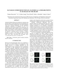
MOLECULAR IMAGING IN BIOINFORMATICS - Pattern Recognition ...

Literature Study
MOLECULAR IMAGING
IN
BIOINFORMATICS
Exploring Interdisciplinary Connections
February 11, 2008
Bioinformatics
Information and Communication Theory Group
Delft Technical University
Laboratory for Clinical and Experimental Image Processing (LKEB)
Radiology
Leiden University Medical Center
Author:
Supervisors:
Martin Wildeman
Prof. dr. ir.M. J. T. Reinders
1047973 Dr. ir. B. P. F. Lelieveldt

Contents
1 Introduction 7
2 Molecular Imaging 9
2.1 About Molecular Imaging . . . . . . . . . . . . . . . . . . . . . . . . 9
2.2 Novel contrast mechanisms . . . . . . . . . . . . . . . . . . . . . . . 9
2.2.1 About Reporter Genes . . . . . . . . . . . . . . . . . . . . . 10
2.2.2 Direct and Indirect Protein Detection . . . . . . . . . . . . . 11
2.2.3 Reporter Gene Applications . . . . . . . . . . . . . . . . . . 12
2.2.4 Current Limitations on Reporter Genes . . . . . . . . . . . . 13
2.3 Molecular Imaging Modalities . . . . . . . . . . . . . . . . . . . . . 15
2.3.1 Nuclear Imaging . . . . . . . . . . . . . . . . . . . . . . . . 16
2.3.2 Computed Tomography . . . . . . . . . . . . . . . . . . . . . 18
2.3.3 Magnetic Resonance Imaging . . . . . . . . . . . . . . . . . 18
2.3.4 Optical Imaging . . . . . . . . . . . . . . . . . . . . . . . . 20
2.3.5 Ultrasound Imaging . . . . . . . . . . . . . . . . . . . . . . 23
2.4 Acquisition Challenges . . . . . . . . . . . . . . . . . . . . . . . . . 23
2.4.1 Quantification of BLT and FMT . . . . . . . . . . . . . . . . 23
2.4.2 Combining Information: Multi-modality fusion . . . . . . . . 25
2.4.3 Combining Information: Follow Up Registration . . . . . . . 27
2.4.4 Current Limitations in Molecular Imaging . . . . . . . . . . . 27
3

3 Molecular Imaging as extra data source for model generation 29
3.1 Acquisition of Spatiotemporal Gene Expression Data . . . . . . . . . 30
3.2 Inferring a Quantitative Model using Spatiotemporal Protein Expression 32
3.3 Quantitative vs. Qualitative Network Models . . . . . . . . . . . . . 34
3.4 Modeling pathways using time series expression data, using conventional
micro-array data . . . . . . . . . . . . . . . . . . . . . . . . . 36
3.5 Discussion . . . . . . . . . . . . . . . . . . . . . . . . . . . . . . . . 39
3.5.1 General . . . . . . . . . . . . . . . . . . . . . . . . . . . . . 39
3.5.2 Creating models for whole body imaging data . . . . . . . . . 40
4 Molecular Imaging as a means for hypothesis testing 45
4.1 Gene Tracking . . . . . . . . . . . . . . . . . . . . . . . . . . . . . . 45
4.2 Cell Tracking . . . . . . . . . . . . . . . . . . . . . . . . . . . . . . 46
4.3 General signal detection and limitations . . . . . . . . . . . . . . . . 47
4.4 Discussion . . . . . . . . . . . . . . . . . . . . . . . . . . . . . . . . 49
5 Discussion 51
5.1 Advantages of MI for the field of bioinformatics . . . . . . . . . . . . 51
5.2 Current Issues and Challenges . . . . . . . . . . . . . . . . . . . . . 52
5.3 Conclusion . . . . . . . . . . . . . . . . . . . . . . . . . . . . . . . 54

Abbreviations
In this paper, a lot of abbreviations are used. For readability, a list of abbreviations is
listed here:
• AFP - Auto Fluorescent Protein
• BLI - Bioluminescence Imaging
• BLT - Bioluminescence Tomography
• BRET - Bioluminescence Resonance Energy Transfer
• (C)CCD - (Cooled) Charge-coupeld Device
• CRET - Chemoluminesce Resonance Energy Transfer
• CT - Computed Tomography
• (D)BN - (Dynamic) Bayesian Network
• ES Cell - Embryonic Stem cell
• FMI - Fluorescence Molecular Imaging
• FMT - Fluorescence Molecular Tomography
• FRET - Fluorescence Resonance Energy Transfer
• GOI - Gene of interest
• GFP - Green Fluorescent Protein
• MI - Molecular Imaging
• MRI - Magnetic Resonance Imaging
• NMR - Nuclear Magnetic Resonance
• PET - Positron Emission Tomography
• SNR - Signal to Noise Ratio
• SPECT - Single Photon Emission Computed Tomography
• WT - Wild Type
• YAC - Yeast Artificial Chromosome
5

CHAPTER 1
Introduction
In this literature study, results are presented of research that was done to identify possible
connections between two fields of research; bioinformatics and molecular imaging.
To be able to study potential connections, the possibilities, limitations and pitfalls of
both fields were studied. Existing techniques of both fields were then translated and
interpreted to possible connections to the other fields.
To be able to study the two fields, it is first important to give a definition of both fields
as how they will be used in this paper.
Firstly, the term bioinformatics in this study has been narrowed down to the definition
of computational biology, as given by the NIH: Computational Biology is “the
development and application of data-analytical and theoretical methods, mathematical
modeling and computational simulation techniques to the study of biological, behavioral,
and social systems” [1].
Secondly, the term molecular imaging in this study is defined as ”the in vivo characterization
and measurement of biological processes at a cellular and molecular level in a
noninvasive manner”. In this paper the term will mainly indicate to the field of small
animal whole body molecular imaging.
Recent developments in molecular imaging have made it possible to visualize gene
expression in vivo. It has thereby become possible to acquire data sets that cover gene
expression in time and in space. This new data could be useful for computational
biology, but how it can be used is a topic of research. Also some analytical tools could
be useful, to aid the research that is currently done with molecular imaging, and change
qualitative interpretations of data that are mostly given nowadays, into statistical sound
quantitative measurements.
This paper is divided into five chapters, including this introduction. First an overview of
background knowledge, needed to study possible connections between the two fields,
is presented in Chapter 2. After the basics of biology and molecular imaging have been
7

Chapter 1. Introduction
covered, a study on existing techniques from computational biology is presented in
Chapter 3, including possible applications to the field of molecular imaging. In Chapter
4, a step into current visualizations in molecular imaging is covered, including a review
on how statistical tests can be applied to these visualizations. In the last Chapter, a
discussion will be presented were global concepts and challenges are presented.
8 Martin Wildeman

CHAPTER 2
Molecular Imaging
2.1 About Molecular Imaging
Molecular Imaging can be defined as the in vivo characterization and measurement of
biological processes at a cellular and molecular level in a noninvasive manner. Molecular
Imaging is a relatively new imaging paradigm that instead of looking at macroscopic
physical processes, sheds light onto biological processes. This field of research has its
roots in the field of nuclear medicine, where images are acquired with Positron Emission
Tomography (PET), by using radio labeled tracers. These tracers are injected into
patients to visualize components of interest. The main advantages of molecular imaging,
compared to other imaging techniques such as cryosectioning, are that biological
processes can be measured in the same animal throughout the whole process of study.
This way, with follow up studies in time, it is certain that the same process is observed
and studied and thus no correction due to differences in anatomy between organisms, is
needed. Furthermore less animals are sacrificed, compared to invasive studies, which
is an improvement from an ethical point of view.
Two developments have made it possible for Molecular Imaging to emerge. Firstly new
contrast agents have been developed, which make current modalities from medical
imaging able to be used for detecting molecular processes. This will be covered in
section 2.2. Secondly, imaging devices have been miniaturized, which allows for small
animal research and thus introduces molecular imaging to the pre-clinical and research
laboratories. This will be discussed in section 2.3.
2.2 Novel contrast mechanisms
With the advent of new specific contrast agents, the field of molecular imaging has
boosted. Based on new, advanced biological insights it has become possible to con-
9

Chapter 2. Molecular Imaging
struct probes that bind to specific biomarkers. Biomarkers are proteins that are specific
for some type of tissue or disease. Contrast agents can be fused to proteins directly.
They can be fused to for instance monoclonal antibodies, to bind to specific receptors
that are for example uniquely expressed in certain tissue cells. Also methods exist
to encapsulate contrast agents in carrier proteins. In molecular imaging, specific
molecules, cells or tissues are visualized by means of these contrast agents. To be able
to do so, four basic criteria for these contrast agents always have to be met: The affinity
of the molecular probe has to be high and specific enough, so it can discriminate between
different cell types. The probe has to be able to cross all kinds of barriers, such
as the blood-brain barrier, so it is diffused homogeneously throughout the body, or at
least the ‘spread function’ of the diffusion has to be known, so it can be corrected for.
The contrast agent needs the ability to be amplified and the acquisition devices must be
sensitive enough to measure the low concentrations of the contrast agents [2].
In the last decades it has become possible to visualize gene expression in vivo by the
use of reporter genes. These reporter genes are in fact contrast enhancers for a specific
modality. Reporter genes are used in nuclear imaging and optical imaging, but also
techniques have been developed for magnetic resonance and ultrasound. These new
contrast agents enables the study of gene expression in a spatiotemporal dimension
which give an advance over the traditional use of micro-arrays, which are currently
used for measuring gene expression, because micro-arrays only allow for temporal
expression profiles. No spatial component is possible with micro-array measurements,
because micro-arrays measure RNA concentrations in a solution, extracted from animal
tissue, which basically gives an average expression level as a result. The only way to
incorporate some qualitative spatial expression profile in micro-arrays, is to make use
of sectioned tissue profiling [3]. This literature study will mainly focus on the topic of
reporter gene expression and measurements in molecular imaging.
2.2.1 About Reporter Genes
The purpose of reporter genes is to make invisible gene expression visible. Also
substrate-protein and protein-protein interactions or other molecular events that are
normally not visible may become detectable in an indirect manner. When using reporter
genes it is important to keep in mind that the genes that are detected are not the
compound of interest, but that the measurements are expected to be directly correlated
with these compounds. In this way information on non detectable processes can still
be acquired. In Bright Field Microscopy and (Laser Scanning) Confocal Microscopy
it already was possible to directly view gene expression by tagging proteins with auto
fluorescent protein (AFP) genes. A lot of research has been done on these AFPs and
currently a range of dyes with an emission wavelength between 500 and 950 nm is
available.
Another gene used as a reporter is found the North American firefly or Photinus Pyralis
and it is called luciferase. Luciferase is able to produce light by catalyzing a chemical
reaction with a substrate luciferin and ATP. Luciferase was first used as a reporter gene,
for measuring the concentration of ATP in samples, by using spectroscopic experiments
[4].
Reporter genes can be used to report invisible genes. The way this is done, is that
the reporter gene is expressed at the same time and rate as the gene of interest. The
behavior of the reporter gene is then studied and the results are interpolated to the gene
10 Martin Wildeman

Chapter 2. Molecular Imaging
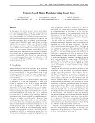
Fig. 2.1: A. The transcription of a gene is regulated by its promoter. To this promoter all kinds
of regulating transcription factors bind with a certain affinity. B If the same promoter is
placed upstream of a reporter gene, then this reporter gene will be regulated by the
same transcription factors as a gene of interest and thus in parallel.
of interest. If a reporter gene is expressed, it is very likely that the gene of interest also
is expressed, of course given that they both have the same promoter (region).
Because reporter genes are heterologous, i.e. they do not occur in the host organism
naturally, they can be toxic to the host carrying it, or in a less severe case affect biological
processes, so that quantitative measurements are not reliable anymore. To minimize
these effects, regulated gene expression is desirable. Alfke et al. gave a proof of concept
where reporter genes were only synthesized at the times that measurements were
needed [5].
2.2.2 Direct and Indirect Protein Detection
A reporter gene can be constructed by cutting the gene out of a source DNA, using
restriction enzymes. If the same promoter as the gene of interest (GOI) is placed upstream
of the reporter gene, the likely effect will be, that transcription of the reporter
gene will be the same of that of the GOI, see Fig. 2.1. When placing a copy of the
promoter upstream of the reporter gene, the only thing that can be said about the GOI
is that it is transcribed. Nothing can be said about post transcriptional effects (for instance
splicing) and whether a gene is translated into an active enzyme or not. Also
caution should be taken when trying to predict the amount of active genes (proteins)
that are formed, because transcription of a gene and translation into a protein do not
always relate one to one.
It is also possible to construct proteins with reported genes fused to it. This way the
genes of interest can be directly observed [6]. These so called fusion proteins are
inserted into the genome by using standard recombination techniques. GFP proteins are
considered to be non toxic, but it has to be mentioned that altering proteins by fusing a
GFP to them, may alter their functionality or influence post translational alterations.
A gene can be copied by using a technique called Polymerase Chain Reaction (PCR).
To do this, the right primers have to be constructed. Primers are short complementary
RNA strands that have sufficient binding energy at certain temperatures to have a starting
point for DNA-polymerase to start transcription. If enough DNA of transcripts and
vectors is produced, then ligands can be made, which in turn can be transfected into
host cells. It is also possible to directly insert the DNA into undifferentiated embry-
Martin Wildeman 11

Chapter 2. Molecular Imaging
onic stem cells (ES cells) and apply recombination. In this way specific genes can be
replaced with (non)functional genes or they can be deleted (knockout).
It is important to emphasize that most reported genes provide an indirect measuring
technique and that detection of those genes are thus not the detection of a functional
gene of interest, but merely an indication that the genes downstream of the same reporter
as the measured protein (among which the GOI) are transcribed.
2.2.3 Reporter Gene Applications
With the ability to synthesize gene constructs that can be measured, the question arises
on what we want to measure. There are two things that can be measured with reporter
genes, of which the first is the existence and amount of a cell being of a certain genotype
and the second one is the measurement of expression levels of a certain gene.
In the first case, a reporter gene is placed in a construct such that it is positioned downstream
of an ‘always on’ promoter, mostly being a viral promoter such as SV40 or
CMV, and thus constantly synthesized in a cell. If the rate of synthesis within the cell
is known, and thereby also the concentration of reporter gene protein within a cell and
the amount of photons per cell per second is known, then the number of cells observed
can be quantitatively be determined. This fact can be exploited to for instance determine
how fast a tumor is growing over time and if, when and where it is metastasizing.
Also infection processes of viruses, bacteria or parasites can be studied, as will be discussed
in Chapter 4. This technique needs the ability to introduce gene constructs into
cell lines.
In the second case, the reporter gene is placed downstream of the same promoter as
a gene of interest. This gives the ability to study gene regulation within an organism.
With high throughput studies, this would allow for spatiotemporal gene expression
studies and thereby act as data source for gene regulatory network inferring as will
be discussed in Chapter 3. Measuring gene expression profiles needs the ability to
generate transgenic model organisms.
There are several techniques for introducing foreign DNA into animal cells. In cultured
cells micro-injection can be applied. In in vivo cases, DNA can be introduced by
particle bombardment. Both methods are called direct DNA transfer. Also transfection
is possible, and the last method of introducing foreign DNA is by use of transduction,
with the use of retro-viruses. Gene therapy for instance is based on this transduction
method. The most used technique for producing transgenic mice, is to inject DNA into
the pro nucleus of a fertilized egg [7]. A targeting vector with an inserted promoter
and reporter gene is transferred to the DNA of the recipient cells and a small percentage
of these cells will have the new gene incorporated into their genome. The number
of gene copies is not always the same and the copy number varies from a few to hundreds
inserted pieces of DNA. Also YAC vectors are used because they can carry larger
strands of DNA and are thus able to express larger, more complex proteins. For GFP
and Luciferase though, the SV40 vectors suffices [8]. For generation of genetically
altered mice, most commonly micro-injection in blastocysts is applied, which gives at
first chimeric mice as a result. This is because the ES cells in the Blastocysts will be
original and transformed ES cells. If offspring of these mice have the same genes it
will be homozygous. A schematic overview is given in Fig. 2.2.
There is a difference between transient and stable transfection. When inserted genes
12 Martin Wildeman

Chapter 2. Molecular Imaging
Fig. 2.2: Constructed genes are purified and inserted into oocytes. Then a selection is made
out of born mice [9].
are inserted into the genome, by making use of a recombinase, the inserted genes will
be expressed stably, but when new DNA is inserted extra-chromosomal, the inserted
DNA will be degraded over time, because it will not be replicated. For temporal gene
expression measurements, stable transfection is needed, also to be certain that each cell
will contain the same genome.
2.2.4 Current Limitations on Reporter Genes
Gene Transfer Reliability
Transfection is not always effective or efficient. The undetermined gene insertion copy
number, mentioned before, makes it impossible to do a quantitative analysis on gene expression.
When multiple copy-numbers are present, this will result in more translation
and thus in more gene expression. To make things worse, copy number and expression
profiles are not always one to one related [10]. With most DNA transfer techniques it
is difficult to predict side effects based on the location where the DNA is transfected.
For example many non coding RNA’s (ncRNAs) have an unknown function and it is
expected that many ncRNAs are not (yet) known. The size of ncRNAs varies from 20
(microRNA) to thousands of nucleotides [11]. Random insertions therefore can give
unpredicted results.
With a technique called Flp-in from Invitrogen, it becomes easier to insert genes into
a genome. The problem to be solved for this Flp-in technique is to produce a stable
cell-line which contains only one Flp site and that seems to behave like a normal cell
line (the long term side effects of DNA insertion cannot be predicted), but once such a
cell line is generated, virtually every gene can be inserted into the Flp system, by using
homologous recombination [12]. Using a Southern-blot it can detected whether there
is one and only one copy of the inserted Flp site [13].
This technique is mostly used to generate on demand genetically altered cell lines.
When cell lines carrying this Flp-in site are transfected with an always on promoter
Martin Wildeman 13

Chapter 2. Molecular Imaging
and a reporter gene, these cells become trackable with FLI, BLI or any other probe
gene. Note that it is only possible to track the cells and keep track of the number
of cells (quantification). No gene regulation can be monitored using this ‘always on’
technique. This tracking is important for temporal study of for example tumor growth
and metastasis, or tracking of infectious agents such as viruses or bacteria, as will be
discussed later.
As long as the regulatory effect of non-coding elements is not completely understood,
it cannot be guaranteed that an insertion has no effect, but if a stable cell line with
a Flp insertion is used, it is relatively certain that new insertions at that site have no
side-effects on the normal functioning of the studied organism or cell line.
Diffusion Coefficient
When measuring reporter gene concentration it is important to keep in mind that the
genes that are measured probably have the same rate of synthesis, due to the same
promoter region, but it is not likely that they have the same degradation rate. With the
basic conversation law it can be shown that proteins with a faster degradation rate will
appear in a lower concentration than proteins with the same rate of synthesis, but a
lower degradation rate.
The general formula of gene formation can be stated as follows:
( )
time rate of change
of protein conc.
= Regulation + Diffusion + Decay (2.1)
The only part in this equation that is equal between the gene of interest and the reporter
gene, is the regulation part. The level of decay and the diffusion coefficient differ. This
has as effect that the protein concentration of the gene of interest cannot be determined
by the measurement of protein concentration of the reporter gene. Something qualitative
can be said about upregulation or downregulation, but quantitative measurements
on up or down regulation are not possible if the diffusion and decay parameters are
unknown.
Post Translational Effects
In addition to these unknown diffusion parameters, it should also be taken in consideration
that the fact that a gene is transcribed, does not guarantee that the protein is
actually formed, or if it is formed, that it will be in a functional shape. Transcribed
RNA in eukaryotes is often spliced into so called coding DNA (cDNA). This cDNA
determines what the amount and order of amino acids in a protein will be. One single
strand of translated messenger RNA (mRNA) can be spliced in different ways, so that
isoforms of the same gene can appear. This also results in different forms of proteins.
With reporter genes it is not possible to identify different protein isoforms. Alternative
splicing is thought to be one of the most important components of the function
complexity of the human genome. Given that different isoforms may be possible for
different regulation effects and that genes can code for up to 40,000 protein isoforms
at least some caution should be taken when interpreting gene expression data [14]. For
different forms of splicing, see Fig. 2.3.
14 Martin Wildeman

Chapter 2. Molecular Imaging
Fig. 2.3: Different splicing effects are possible. a: exons can be included or excluded, and
splice sites can be altered. b: Initiation of translation or stop signals can be altered and
inframe deletions or insertions are possible [14].
Fig. 2.4: Many modalities from clinical imaging have been miniaturized for the use in Molecular
Imaging [16]
Protein Tagging
When protein tagging is possible, it is relatively certain that the molecule that is visualized
is the same as the gene of interest. For tagging genes the main reporter genes
that are used, are the GFP family proteins. Although these genes are thought to be non
toxic, it should be taken into account that gene tagging may alter the functionality of
proteins and thereby may cause the alteration of biological regulation and functioning
in the studied organisms [15]. In biological processes everything is based on equilibria
and minor distortions may cause great effects.
2.3 Molecular Imaging Modalities
Besides the upcoming of in vivo gene reporters, another trend seen in the field of molecular
imaging is that detection devices have been miniaturized. These micro devices are
cheaper than their clinical counterparts and allow for small animal whole body imaging
[16]. Because these new acquisition devices are smaller, some scaling problems need to
Martin Wildeman 15

Chapter 2. Molecular Imaging
be tackled, for instance how much resolution is needed to get meaningful information
and what the measured volume must be [2].
Commonly seen reporter genes in short can be divided into three imaging modalities:
Radio-nuclide imaging, optical imaging and magnetic resonance imaging. Each
category has its own advantages and disadvantages in terms of resolution, sensitivity,
acquisition time and substrate admission [16]. In Molecular Imaging also the modalities
CT and Echography can be used, but because they cannot or can hardly be used
for visualizing gene expression, they will be discussed in less detail in this literature
study. It should be noted though that CT may give much extra information as an underlying
modality if extra resolution or spatial context is required. To be able to use this
information, image registration is needed, as is discussed in section 2.4.2.
Most imaging modalities seen in medical imaging can be used in molecular imaging,
with appropriate contrast agents. The modalities nuclear imaging, radiography imaging,
magnetic resonance imaging, optical imaging and ultrasound imaging will be described
shortly. For each modality a reporter gene, if applicable, and a short description
of acquisition will be given. For all modalities hold the same arguments; if a contrast
enhancer can be bound to a molecular probe, it is, given that it is not toxic and that it
can pass all necessary barriers, suitable as an (indirect) reporter for gene expression. A
short overview of different modalities and their general specifications is given in table
2.1.
2.3.1 Nuclear Imaging
Nuclear Imaging is based on unstable molecules that emit positrons or γ-rays and
thereby fall into a more stable energy state. Two modalities are seen in molecular
imaging, namely PET and SPECT. In PET, most used isotopes are 15 O, 13 N, 11 C and
18 F and these isotopes emit positrons. When a positron is emitted and collides with an
electron it annihilates into two γ-rays which travel in a ∼ 180 ◦ direction. In PET, these
γ-rays are then collected and converted to a visible image, by making use of a ring
of gamma detectors. Due to the fact that the γ-rays are traveling on one line and due
to attenuation in the different tissue types, the exact location of the positron emitting
source can be located in the 3D space [16]. Coinciding photons in the detector ring are
from the same source (See Fig. 2.5).
Isotopes used in SPECT are 123 I and 99m Tc emit γ-rays [19] which do not simultaneously
travel in opposite direction. It is thus not possible to use a detector ring to pinpoint
the location of the source of emission. Instead of using a detector ring, γ-rays are
detected by special camera’s, that consists of a pinhole collimator, a scintillating crystal
and a photon detector. γ-rays are converted to photons in the visible frequency range
by the use of scintillating crystals and thereafter are detected by the photo detectors.
By making use of pinholes, only photons flying on a line parallel to the pinholes/septae
are detected. Knowing that captured γ-rays can only come from the source directly, a
line in 2D space where the source must lie on is known (Fig. 2.6). When rotating the
camera around the sample, it is possible to reconstruct 2D images. The technique of
SPECT therefore is comparable to CT, but different energy photons are used. Multiple
2D images acquired with SPECT, can be reconstructed to a 3D model the same way as
in CT as will be seen later.
Sensitivity of SPECT is of an order of magnitude lower than what can be achieved with
16 Martin Wildeman

Chapter 2. Molecular Imaging
Fig. 2.5: PET tracers are injected into organism. A PET tracers contain atoms that are unstable
and emit positrons. If these positrons collide with electrons, they annihilate into two
γ-rays traveling in opposite direction. To measure gene expression, reporter genes are
used that can accumulate PET tracers in a cell, so that these cells become visible.[17,
18]
Fig. 2.6: SPECT is based on pinhole detection. PET is based on coincidence events.[19]
Martin Wildeman 17

Chapter 2. Molecular Imaging
PET. This is due to the fact that in SPECT, γ-rays have to be tunneled through septae in
a lead barrier, so that only straight traveling rays are detected. The longer these septae
are, the higher the resolution in SPECT becomes, but also the less sensitive. (Less rays
are detected, because more are shielded.) An advantage of SPECT over PET is that the
used tracers have a longer half life. This allows for studies on slower/longer biological
processes. The biggest disadvantage of SPECT is its lower (but still good) sensitivity
compared to PET.
The reporter genes for PET are genes that have an high binding specificity for some
radio labeled biological molecules. These substrates are normal substrates labeled with
positron emitting isotopes. To make sure that the overall criteria are met, specifically
barrier crossing, it is important to use a molecular target that is expressed on the surface
of a cell, a so called cell surface protein, or to make use of a molecular probe that can
freely pass the cell membrane (For example see [20]). If the probe can pass the membrane,
it is important that it is ‘trapped’ inside the cell, after some chemical reaction, so
it accumulates inside the cell. It is important that the cell is not killed by this (toxicity),
but accumulation of the radioactive compound inside the cell causes a higher signal.
Also the use of monoclonal antibodies, to detect certain cell types is possible [21].
2.3.2 Computed Tomography
By making use of the x-ray wavelength region, the detection of heavy atoms, such as
calcium atoms, is possible, because the attenuation of x-rays is different for different
weight atoms.
By rotating the sample or the scanner, multiple projections of the sample can be obtained
(See Fig. 2.7). The scanned sample can be reconstructed slice by slice, where
multiple projections of a slice are backprojected to obtain a 2D image. The projections
can be filtered before backprojection, to include or occlude certain frequencies. Heavy
atoms cause more attenuation than light atoms and thereby sensitive for difference of
(average) atom weight in tissues. Positions of heavy atoms, or contrast agents, can be
reconstructed by making use of this backprojection algorithm. The resolution of CT is
limited by the ionizing effect of x-rays. This effect causes direct radiation damage and
in the longer term DNA damage. To obtain a higher resolution, more rays per voxel are
needed, which causes more damage and this damage needs to be minimized.
Gene reporting probes, to be detectable, need to contain heavy atoms. The effect of
large quantities of these substrates are not known and CT is not used as a gene expression
measurement. X-ray imaging, and especially computer tomography (CT), are
currently mainly used as a structural modality in MI. By making use of modality fusion,
expression data can be fused into a high resolution spatial context.
2.3.3 Magnetic Resonance Imaging
Nuclei are brought into alignment by a strong magnetic field. They can have a high
energy spin, when the poles of nuclei are the same as in the magnetic field and a low
energy spin when the poles are oppositely aligned. All elements with a nucleus that has
an odd amount of nucleons, being protons and/or neutrons, can be used form MRI. To
be more precise, every nucleus that contains an unpaired proton and/or neutron is suitable
for MRI. Nuclei that are most commonly used are 1 H, 2 H, 31 P, 23 Na, 14 N, 13 C and
18 Martin Wildeman

Chapter 2. Molecular Imaging
Fig. 2.7: Multiple 2D x-ray images of a body are acquired using different rotations. With a set of
these images a 3D space can be reconstructed. (kabayim.com/images/spiralCT.jpg)
19 F. Every isotope that has a non zero nuclear spin can be used for Nuclear Magnetic
Resonance. Once all nuclei are aligned into the magnetic field, a RF pulse is generated
by placing a current through a coiled wire around the sample. This pulse causes the
nuclei to be brought out of alignment of the static magnetic field. After this, the spins
are returning into alignment with the static magnetic field and the duration needed for
this realignment, called the spin relaxation times, are measured. This can be done by
the same coil or by an additional electromagnetic coil.
The location of the molecules can be determined by placing a gradient in the force of
the static magnetic field. This is because the frequency of the spin is determined by the
force of the magnetic field, as is shown in equation 2.2.
ω 0 = γB 0 (2.2)
Only nuclei that have the same frequency (ω 0 ) as the RF signal, will respond to this
signal. This is why the technique is called Magnetic Resonance. B 0 is the force of the
magnetic field in Tesla and γ is the gyromagnetic ratio, which is a specific property of
the nucleus.
There are different relaxation phases, T 1 and T 2 that correspond to the Z and the X-
Y plane respectively, and although these differences are quite fundamental, they are
considered to be out of scope of this study.
The measured relaxation times are mainly determined by the chemo-physical environment.
The combination of all measured relaxation times results in a NMR signal in the
time domain. This signal can then be converted into a frequency domain by applying
a Fourier transform [16, 22]. MR is very sensitive to differences in soft tissues. Extra
contrast agents, such as gadolinium or dysprosium can be used to enhance the MR
signals in regions of interest.
MR is not yet really used for imaging of gene expression, because of its lack of sensitivity
to small amounts of reporter genes. With appropriate amplification strategies
though, it is possible to obtain enough signal and with MR very high resolution can
be achieved. Louie et al. developed a shielding container that is able to ‘switch off’
gadolinium. In the presence of β-Gal, which is the protein produced by the LacZ gene,
Martin Wildeman 19

Chapter 2. Molecular Imaging
Fig. 2.8: Gadolinium encapsulation is cleaved by β -galactosidase at the red bond shown in A.
This way the Gd 3+ becomes detectable by MRI once it gets in contact with water. Left
is the intact cage and right is the cleaved cage where gadolinium is free. (A) shows the
chemical geometrical structural formula and (B) shows the same molecules in a space
filling model. The purple atom that can be seen in (B) right, is the free gadolinium atom
[23].
this shielding container gets cleaved in such a way that a coordination site at the Gd 3+
becomes free and gets ‘activated’ (see Fig. 2.8). The activated Gd atom generates a
roughly twofold stronger signal than the inactive Gd. Furthermore MR does not suffer
from limitations that are seen in optical imaging, concerning spatial reconstruction
algorithms. [23]
MRI is still mainly used in MI as an extra structural modality for modality fusion. Also
combined PET-MRI scanners exist, but combined PET-CT scanners are more common.
2.3.4 Optical Imaging
Optical imaging makes use of the frequency spectrum in the range of visible and near
infra-red light. Images are acquired by using basic CCD Cameras. Photography in
the clinical field was mainly used for showcases of phenotypic effects of diseases or
injuries, mainly for educational purposes, but with the upcoming of optical contrast
agents, it is now possible to use this modality as a molecular imaging modality. An
important development for this to be possible is the availability of more sensitive cameras.
The technique of these cameras is the same as normal CCD cameras, but they
are cooled down. The technique is called CCCD (Cooled Charge Coupled Device) and
enables that light sources with a really low intensity can still be detected.
20 Martin Wildeman

Chapter 2. Molecular Imaging
Fig. 2.9: Schematic overview of different capturing techniques. a and b are planar imaging c is
the principle of tomography. d is a reconstructed result of optical tomography, of which
the emission source has yet to be calculated [25].
Fluorescence Molecular Imaging
The most common Auto Fluorescent Proteins are the eGFPs (enhanced Green Fluorescent
Proteins). These proteins must be excited with an outside light source, the
excitation beam or source. An AFP must be exited with an higher energy than that it
emits. Therefore, with appropriate filtering, emitted light can be filtered out for imaging.
In this way only the light that has its origin from the AFPs is recorded. This is
done because noise from other homologous AFPs might give interference because of
overlapping spectra. With FMI, images can be acquired in a planar form, resulting
in a 2D image, or by using a technique called optical tomography, where a 3D image
can be acquired. The penetration depth for tomography is much higher than for planar
imaging, but planar imaging has the possibility for much higher throughputs [24]. A
short schematic view of different capturing techniques is given in Fig. 2.9.
Bioluminescence Imaging
When bioluminescent proteins, of which luciferase is most common, are present in
an organism, an image of the gene expression can also be made with a Cooled CCD
Camera. This is called bioluminescence imaging. Although the emission intensity
of light in BLI is much lower than in FMI, it has a much higher sensitivity. This
is because there is less background signal in BLI. The only sources of light are the
proteins itself [25]. Bioluminescent sources can be detected by using a very sensitive
camera, combined with a dark chamber in which no other photons are present than the
photons of the bioluminescent protein. A schematics overview of steps needed for BLI
is shown in Fig. 2.10.
Protein-protein interaction with FRET, BRET and the yeast two-hybrid system
GFP and Luciferase can also be used to measure protein-protein interaction, by making
use of a phenomenon called FRET or BRET [27, 28]. It is currently possible to
visualize Protein-Protein interaction [29]. This is done by the use of fusion proteins.
Copies of genes are inserted into the organism of interest. With FRET two GFPs and
Martin Wildeman 21

Chapter 2. Molecular Imaging
Fig. 2.10: Schematic of Bioluminscence Imaging. (A.) BLI genes are inserted into cell lines
or DNA constructs, (B.) are then inserted into an animal model (C.) and images are
captured. (D.) Acquired data is then quantified and visualized [26].
Fig. 2.11: Principles of FRET. a,b,If proteins are in close proximity (less than 60 Å) the emission
of the acceptor GFP is measured. Otherwise, only the emission of the donor GFP,
with different wavelength, is measured. c shows some techniques involving FRET
[29].
with BRET a Luciferase and GFP are fused to gene X and gene Y by placing them
downstream of a promoter. When gene X and Y bind, the two GFP’s get in close proximity
of each other, such that resonance energy transfer is possible, as can be seen in
Fig. 2.11. Not only protein-protein activity can be visualized, but also for instance,
protease activity, which can act on a restriction site in the linker DNA of two fused
GFP proteins. With a CCCD camera acquisition is possible. Another method of visualizing
protein-protein interaction is the yeast two-hybrid system. In [30] in a proof of
concept, the interaction of MyoD and ID is visualized. Y2H is an indirect measuring
technique. The interaction of the two proteins of interest induce the transcription of
Luciferase which in turn is translated and can be visualized with a Cooled CCD Camera.
The reporter gene of use can be chosen freely. For the mechanism, see Fig. 2.12
22 Martin Wildeman

Chapter 2. Molecular Imaging
Fig. 2.12: The Yeast Two Hybrid system. Gene X and Y are fused GAL4 and VP16 which
form an active transcription factor [31] for a luciferase gene, by placing the luc gene
downstream of a GAL4 binding site [30].
2.3.5 Ultrasound Imaging
Ultrasound Imaging is based on echo. To obtain an image with ultrasound, short, high
frequency sound pulses are generated. At each barrier where a change of tissue is
located, a portion of the signal is reflected and can be detected by a scanner. The time
it takes for a signal to return to the source, is correlated to the distance that that signal
has travelled. Ultrasound contrast agents are used to enhance the signal. Most common
agents are small air or gas bubbles, called micro-bubbles. Not only do they form a
strong reflective barrier (blood/gas), they also resonate which make them even more
reflective [32]. Micro-bubbles are quantifiable. Although in the traditional ultrasound
resolutions are not really high, with ultrasonic biomicroscopy resolutions of up to ∼
40µm can be achieved and with scanning acoustic microscopy, which is an even higher
frequency sound (200 MHz and higher) resolution of 3 µm are achievable. It should be
noted though that penetration depth decreases with an increase of frequency. With new
micro-bubble contrast agents, specific surfaces can be bound and contrast is enhanced.
Micro-bubbles are encapsulated in a protein and fused to specific antibodies. This
is used for instance, to image inflammatory cells and these specific contrast agents
opens the door for molecular imaging. Ultrasound is not used for gene expression.
This is mainly due to the lack of suitable gene reporters, but also the resolution versus
penetration depth trade-off plays a role. This technique may provide useful information
on concentration flows as will be discussed shortly in 3.
2.4 Acquisition Challenges
2.4.1 Quantification of BLT and FMT
Forward and Inverse Problem
In contrast to PET, for BLT and FMT a scattering and absorption model is required to
be able to solve the inverse problem. Finding the right parameters is called the Forward
Martin Wildeman 23

Chapter 2. Molecular Imaging
Table 2.1: Short list of specifications of different modalities. Source: Molecular Imaging in Living
Subjects, Massoud
problem. E.g. Given the source of emission what must the parameters of the model
be to generate the observed data Once these parameters are estimated, one can try
to solve the inverse problem, e.g. given a model with known parameters and given an
observation, what is the shape, location and density of the emission source For FMT
it is possible to make an approximation of the forward model, because a known input
light source is available, of which the output can be measured. From the attenuation
model, obtained from the known laser light source, it is then possible to start solving
the inverse problem for a fluorescent source. The forward problem cannot be solved
with BLT as no known light source can be used for estimating the parameters of the
model. A priori anatomical information therefore has to be incorporated [33]. To do
that, a second modality, such as MRI or CT is needed to provide anatomical details
about the model. A priori model information can also be obtained from mouse atlas
databases, see Fig. 2.13 [34]. The problem with multi modality though is, that it is not
straightforward to register these modalities on on each other and errors are introduced
because of differences between the model and the atlas.
When registration is complete and successful, different tissues in the model can be
segmented an with those segments the inverse problem can be solved. For the optical
parameters mean values from the literature can be used. To approximate the photon
propagation, the following equation can be used [35]:
{ −∇·(D(x)∇Φ(x))+µa (x)Φ(x)=S(x)
D(x)=(3(µ a (x)+(1−g)µ s (x))) −1 (x ∈ Ω) (2.3)
In this equation S(x) is the unknown source density, Φ(x) is the photon density at
location x. µ a , µ s and g are optical parameters. In the paper of Cong [35] equation 2.3 is
solved using a modified Newton method. But it is also possible to use a MAP approach
[33]. It is proved that this inverse problem has a unique solution [36], provided that the
model is well enough defined.
Resolution Improvement
A problem concerning the ill-posedness in BLT is that the optical parameters of the
body tissue are temperature dependent [37]. This temperature dependency can be mod-
24 Martin Wildeman

Chapter 2. Molecular Imaging
eled, but this is at the cost of an even more complex model and thus at the cost of extra
computational power. A higher resolution and more accurate result will be gained by
adding this temperature dependency. It should also be noted though that temperature
has to be measured for every tissue which will likely introduce a new inverse problem
for the infrared spectrum.
Chaudhari et al [38] propose to use spectral information for reconstruction of a BLI
source. Because of attenuation in the body tissues, there is a spectral shift in the signal.
By capturing hyper-spectral ( 100 spectrum bins) or multi-spectral( 10 bins) these attenuation
differences can be taken into account. This way, two overlapping sources in
a 2D image of which one is superficial and one is located deeper, can be distinguished.
It should be noted that for each spectral band, an individual inverse problem has to be
solved.
Backprojection
It remains to be seen whether these complex optimization problems are useful. The
optical properties of different tissues in the small animal models are unknown and simplified
assumptions are used for the reconstruction of the BLT energy source [39]. The
most important question for combining BLT (or Fluorescence Tomography for that
matter) and the field of Systems Biology will be: How much resolution in space and
time is needed, for cell specific and process dynamic behavior respectively, for feasible
application of molecular imaging to track gene expression in the organism In the
paper of Kok [39] a relatively straightforward algorithm is used for reconstruction of
the bioluminescent source. Scattering is not taken into account and the tissue structure
is assumed to be homogeneous, which is clearly not the case. Despite these simplifications
a good estimation is achieved for source localization of superficial lesions.
Combined with the fact that the authors only want to attract attention to a location in
the accompanying CT (or another structural data-file), the algorithm can be seen as
an efficient and simple reconstruction algorithm. The authors use a backprojection of
eight planar images, each rotated a known number of degrees, onto a ‘3D’ structural
data set. This methods provides good resolution for superficial BLI sources, but has
lower resolving power for deeper lying tissues. It is also shown though in [40] that also
with coarse grained resolutions interesting new information can be obtained from gene
expression data.
2.4.2 Combining Information: Multi-modality fusion
Because different modalities contain different information it is useful to combine this
information. CT for example is sensitive to elements with a high atomic number, for
example calcium which is found in bones and calcification. Heavy atoms such as iodine
can be injected in the blood stream as contrast agents making veins and blood-rich
organs detectable. MRI on the other hand is very powerful for visualizing different soft
tissues. When these two modalities are correctly combined, they support each other
and fill in tissue differences that the other modality it not able to detect.
Bioluminescence and Fluorescence planar images by themselves don’t give much detail
on the location of gene expression. This is due to diffusion and scattering inside the
body, before photons reach the surface of the body (e.g. the skin of the mouse) from
Martin Wildeman 25

Chapter 2. Molecular Imaging
Fig. 2.13: Mouse atlas with a surface rendering of skeleton and different organs [34].
which the picture is taken. As an effect only a rough indication (in terms of millimeters)
of the location can be given based on the set of 2D images. A huge advantage of BLI
and FMI though, is that they are much more sensitive to abnormalities than the existing
medical imaging modalities. Therefore it is possible to detect diseases, well before
morphological changes are observable. If a detection is made with BLI or FMI, other
modalities can be used to study morphological changes in detail at the specific sites of
interest [39].
How to align different modalities The position of the mouse model during the acquisition
of different modalities most likely differs. If the two modalities are combined, a
reconstruction of the source will be possible. For the combination of multiple modalities
though, alignment by image registration is needed. This 3D alignment is not a
straightforward procedure [16]. If all modalities can be aligned to a standard atlas, this
way modalities can be fused. In the paper of Baiker [41] a registration of the skeleton
is automatically done based on an optimization, that minimizes differences between
an mouse skeleton atlas and a skeleton generated from a CT scan. By extending this
work, it is also possible to register some marks on the mouse skin and combined with
the skeleton information, interpolate where the organs of the mouse are located. It is
also possible to generate a 3D image from structured light from planar images. By
combining those models, is should be possible to estimate where different tissues in
the model are located.
It is important to notice that a mapping to an atlas is needed for both qualitative as
quantitative gene expression measurements [42]. To be able to tell in which organ gene
expression occurs for instance, one has to know where the organs are located in the
3D space of an organism first. A whole range of mouse atlas databases currently is
available [34]. Few of them also contain spatiotemporal gene expression data (Mouse
Atlas Project developed at the University of Edinburgh and DigiMouse), to which new
measurement can be correlated. [43, 42, 34]
26 Martin Wildeman

Chapter 2. Molecular Imaging
2.4.3 Combining Information: Follow Up Registration
Although in vivo imaging allows for continuous measurements in time without moving
the animal, most if not all diseases that are studied have a progression in terms of
weeks rather than in terms of hours. It is therefore infeasible to continuously maintain
the studied animal at the exact same position and it is thus necessary to be able to
register images of the same animal in individual experiments.
For follow-up registration, the same atlas approach can be used as for multi modality
fusion. Once it is possible to register the modality on an atlas, it is a small step to
register a ‘time series’ of this same modality to this atlas.
To overcome or prevent some of the registration problems, it is also possible combine
multiple modalities during the acquisition [38]. This way, it is ensured that both
modalities are exactly in the same location in the x,y,z space. Prita Ray et al. [20]
are doing much work on multi modal capturing, by constructing multi modal reporter
genes. In this way FMT, BLT and PET can be acquired with the use of one and the
same reporter gene construct. Also a combined micro PET-CT scanner is used, to
obtain high-resolution anatomical images and gene expression data [44].
In the ideal case, the lab assistant should not need to worry about how to position the
animal for measurements, but positioning the animal in the same way each experiment
makes the registration a lot easier. An effective way to fix the organism in a spatial
context is the use of animal holders. By positioning animals in the same way each
time a acquisition is done, the registration problem is easier solved by reduction of the
degrees of freedom.
2.4.4 Current Limitations in Molecular Imaging
To obtain useful gene expression data with molecular imaging, multiple measurements
have to be made and results have to be combined in one data set. These measurements
contain some noise which introduces inaccuracies, but registration steps will also introduce
new inaccuracies that further decreases the resolution of measurements that can
be achieved. Different kinds of noise are discussed below.
General Noise
Every modality suffers from its own noise problems. The basic problem with noise is
that it can give an overlap with the signal, especially when the signal to noise ratio is not
high enough. To overcome some of these SNR problems, the means of amplifications
of the reporter contrast agents can be used, but if a quantification of gene expression
levels is necessary it must be known how much amplification is used.
Attenuation
Solving the inverse problem is a difficult task. By using the anatomical information
from an atlas, you introduce an error due to the difference between the organism of
study and the reference organism. The optical parameters of the body tissue are temperature
dependent [37]. This temperature dependency can be modulated, but this is
Martin Wildeman 27

Chapter 2. Molecular Imaging
at the cost of an even more complex model and thus at the cost of extra computational
power. Moreover the temperature in an organism is not homogeneous but differs in
space and over time. This will likely affect reconstruction accuracy.
Multi-modality and Follow-up registration
A problem with BLI and FLI, is that it is based on 2D images that only provide pictures
of the surface. It is possible to register CT data to a 3D mouse atlas, and it is also
possible to register 2D BLI data to 3D CT data [39]. Both registration steps introduce
errors. Moreover because it is relatively easy to model rigid conformational changes,
but it is more difficult to model soft tissue deformations. If BLI sources are located in
soft tissues, the reconstruction of the source therefore becomes more inaccurate. In the
ideal case, small animal models are used to be able to mimic diseases in humans, but if
not high enough resolutions can be obtained with small animal models an exploration
to smaller, simpler and transparent organisms can be made, such that the light sources
can be seen directly and therefore reconstruction of the light source, if already needed,
becomes straightforward.
28 Martin Wildeman

CHAPTER 3
Molecular Imaging as extra data source for model
generation
With the ability to visualize gene expression the question arises on what can be done
with acquired data. To answer this question we take a look into the field of bioinformatics
where gene expression data already is analysed.
One reason to strive for an understanding of the underlying cellular processes in an
organism, is to be able to predict it’s behavior and to change or correct its behavior if
needed. To do this, it is not always needed to understand the full functioning of the
system.
There are two approaches for gaining insight in cellular processes. Firstly, by doing
experiments at a low level and secondly by simulating (high level) processes to mimic
observed data. With large complex biological networks possibly only the latter approach
is feasible for obtaining a ‘full’ understanding [45, 40].
In an attempt to relate the field of molecular imaging to the field of bioinformatics,
some examples from bioinformatics are studied and related to MI in this Chapter.
Firstly some studies will be highlighted where spatiotemporal data is acquired using
high throughput techniques, secondly some findings on mathematical models for network
inference will be presented, thirdly a short concept will be given on how to translate
these mathematical models from quantitative to qualitative model, because data
quality is not always good enough for quantitative model construction. Finally a concept
on statistical model inference will be given, based on time series micro array
experiments.
Some findings will then be discussed and questions will be posed in the discussion
section.
29

Chapter 3. Molecular Imaging as extra data source for model generation
3.1 Acquisition of Spatiotemporal Gene Expression Data
In a spatial-temporal gene expression study on Drosophila melanogaster, Seroude et al.
obtained a set of age related genes of which expression changes with age [46]. For the
measurements, extraction and cryosectioning were used for time and spatial expression
profiles respectively. Genes were visualized using the Flytrap system and staining of
β-galactosidase. This way, a 3D+t gene expression profile was obtained. It should be
noted that this experiment was not an in vivo measurement, but the possibility of Flytrap
to express GFP [47] could open the door for non-invasive molecular imaging. In situ
images of the Drosophila Melanogaster could be clustered by using pattern recognition
techniques. In [3] embryo images were studied by using a Gaussian Mixture Model,
an eigenvector basis and a discrete Haar-wavelet as feature space. All pictures were
aligned by making sure that the dorsal side of the embryos was on top and the anterior
on the left. Similar spatial gene expressions were clustered, using graph partitioning.
This way the authors were able to cluster the embryos into different developmental
stages (temporal) and co-regulated spatial expression profiles in those stages (spatial
correlation). Genes with similar expression profiles are thought to be involved in the
same pathway. With this procedure they were able to get a 99,55% staging overlap,
meaning the difference in developmental stage in embryonic development annotated
by the algorithm, compared to expert annotation. This overlap suggests that automated
gene expression measurements are feasible. Indeed in [48] it is said that automatic
high throughput measurements of ISH is feasible and the authors created a mouse atlas
containing spatial gene expression data. Also in their gene expression profile clustering
was done.
The power of spatiotemporal expression measurements is, next to the fact that spatial
information is obtained, that it is sensitive to gene expression in small clusters of
cells. In microarray data these expression profiles would be averaged out by larger
cell clusters with different expression levels [48]. For example, purely hypothetical,
if in a developing embryo there is upregulation in the anterior and downregulation in
the posterior, a microarray experiment would detect no regulation, whereas a spatial
measurement would be able to show this ‘expression gradient’
Dupuy et al. acquired a spatiotemporal gene expression profile by using in vivo imaging
[49]. Because in their paper the authors make use of spatiotemporal in vivo imaging of
which techniques may be extendable to whole body molecular imaging, their publication
is covered in extra detail here.
In their paper Dupuy et al. made a high throughput analysis of about 900 gene promoters.
They used the technique as visualized in Fig. 2.1. Each of those 900 promoters
were expressing a GFP protein and these promoters covered about 5% of the protein
coding genes in C. elegans. Because they wanted to do gene expression measurements
in a developmental study the authors needed some way to incorporate a temporal component
in their spatial gene expression profile measurements.
Temporal arrangement using COPAS
The authors measured gene expression using GFP as a reporter gene and measured
expression profiles on the longitudinal axis of the organism Caenorhabditis elegans.
Instead of measuring expression profiles directly over time, the authors used the body
30 Martin Wildeman

Chapter 3. Molecular Imaging as extra data source for model generation
Fig. 3.1: a Images as captured and converted into a one dimensional GFP intensity bar. b They
are aligned with respect to orientation and length, to get a chronogram c. Then the
chronograms are normalized in time d so that correlation can be calculated [49].
length of the organism as an indication of age. This length could automatically be
sorted by a device called COPAS (‘complex object parametric analysis and sorter’,
produced by a company called Union Biometrica). The working of this device is based
on flow-cytometry which basically separates particles on their size. Larger/heavier
particles will have a longer time of flight than relatively smaller organisms. Images
were acquired with a CCD camera and a confocal microscope. The COPAS system
is able to generate fluorescent emission profiles along the anterior-posterior axis of C.
elegans automatically.
Chronograms
With the large amount of gene expression profiles that were measured this way, the
authors created a set of what they call chronograms. A chronogram is a two dimensional
expression profile, containing a spatial component and a temporal component.
As can be seen in Fig. 3.1 the expression data was converted into intensity bars, based
on the intensity measurements of COPAS. These intensity bars were then aligned and
stacked on top of each other, based on size, as can be seen in Fig. 3.1 c. To be able to
compare the chronograms with other genes, these chronograms were normalized to a
standard chronogram size which contains one line for each size. If no measurements
are available for a certain size an empty line appears in the normalized chronogram.
When multiple measurements are available for a certain size, these measurements get
averaged onto one line in the normalized chronogram (Fig. 3.1 d).
Chronograms that were acquired report the activity of the proximal promoter of 1,610
unique predicted loci, i.e. the promoter was active according to the measurements and
1,610 of those chronograms have only one locus on the chromosome containing the
same promoter region. Roughly 900 measurements contained an average signal that
was above background noise. Most of the other 700 chronograms had a too low intensity,
probably due to an extra-chromosal promoter::GFP construct, a result of limitations
in gene transfer discussed earlier in this paper.
Martin Wildeman 31

Chapter 3. Molecular Imaging as extra data source for model generation
Spatial prior knowledge
The chronograms can be related to tissue specific expression profiles. A gene that is
for example only expressed in the Pharynx has a different ‘fingerprint’ than a gene
that is only expressed in the Gonad sheath. To generate the chronograms, qualitative
tags obtained from microscopy and microarray experiments indicating locations of
gene expression were used and clustered and chronograms from all genes known to be
expressed in the same (qualitative) regions were averaged into one chronogram. The
authors warn that this procedure only gives robust fingerprints for large numbers of
measurements containing the same tag, because many genes are expressed in multiple
regions and with little chronograms to average over, these extra locations may show up
as a signal in fingerprints where they actually do not belong. These fingerprint chronograms,
allow for qualitative location statements on newly obtained chronograms.
Temporal prior knowledge
The same approach was used for expression profiles with known high correlations obtained
from microarray data. These expression clusters obtained from microarray data
did not give clear patterns in the averaged chronograms most of the time, indicating
that co expression in time, measured in microarray data, not necessarily means coexpression
in space. Some examples, such as the ‘neurons’, ‘germ line’ and ‘intestine’
clusters were in correspondence with the associated high correlation in microarray data
though (i.e. a clear expression pattern was seen).
The chronogram promoter activity measurements can be correlated to each other. Chronograms
with high correlation can be clustered and most likely will be functionally related.
To get an event better spatial localization, the authors predict that in the near
future COPAS will be able to generate 3D aligned expression profiles. This, they expect,
will give more accurate four dimensional chronograms, where overlapping organs
will not cause inaccuracies anymore.
To summarize the paper of Dupuy et al. shortly: Age/developmental stage is defined as
the temporal element in the measurements. In this way, high throughput measurements
are feasible, where alignment of the measurements is automatically done. When time
and spatial expression are combined, a so called chronogram is obtained; see Fig. 3.1.
After normalization of these chronograms, they can be correlated and when high correlation
is seen, the function of the proteins measured are likely to be involved in the
same cellular process.
Because Caenorhabditis elegans is a transparent organism, measurements are direct
and precise. Compared to whole body imaging of mice, this could give a problem,
because for each gene a location estimation of expression has to be done.
3.2 Inferring a Quantitative Model using Spatiotemporal
Protein Expression
Reinitz et al. state that to model processes, high detail is not needed. The detail of the
model will just be lower if less detail and lower resolution data is available [40]. In
32 Martin Wildeman

Chapter 3. Molecular Imaging as extra data source for model generation
their work they look at low resolution spatial gene expression profiles to study regulation
effects on eve stripe formation. With a few simplifications, necessary because
of a lack of detailed data, they were still able to construct a model which was capable
of simulating the eve stripe formation. Where Reinitz et al. used only the longitudinal
protein gradients for their model, Krul et al. take the geometrical complexity of
the reality into account [50]. They do this by defining cells as point shaped objects
and the intracellular as the space around it with this space having the shape of the organism,
Drosophila. Krul et al. also simplified the model by only looking at a small
selection of known regulating proteins. With this simplification they were still able to
mimic the systems behavior, but there were deviations due to the simplifications. When
studying the processes in a two dimensional space these deviations became larger. The
model they used consists of the following functions where the difference between intra-
/extracellular and diffusion/non-diffusion is taken into account.
The change over time is described by:
Where h i j =
N g
∑
k=1
δg i j (t)
δt
The extracellular protein concentrations are modeled by:
δc j (x,t)
δt
And equations 3.1 and 3.2 are constrained by:
= φ(h i j)
k j + φ(h i j ) − λ jg i j (t)
W jk g ik + h j and i = 1,..,N c and j = 1,..,N g
(3.1)
= D j ∇ 2 c j (x,t) − λ j c j (x,t) (3.2)
g i j (t) = c j (x i ,t) (3.3)
The symbols in these equations represent: g i j : concentration in cell i for gene j, c j :
extracellular concentration of gene j. λ j : degradation rate of gene j, k j : formation rate
of gene j, h j : activation threshold for gene j and D j : diffusion coefficient of gene j.
W jk contains the regulatory effects of gene j on gene k. It consists of real number values
and these values are positive, negative and zero, for upregulation, downregulation and
no regulation respectively. N c is the number of cells present in the model and N g is the
number of genes incorporated in the model.
Clearly W is the matrix with parameters that we want to estimate, because with these
regulation parameters a gene regulation network can be constructed. Positive or negative
feedback loops for each gene relation are modeled. Also λ,k, h and D are parameters
that need to be set.
Krul tuned or optimized the parameters by hand, to mimic the model. Reinitz et al.
used an optimization algorithm, called simulated annealing, but other optimization algorithms
can be used, such as a genetic algorithm. The cost function they used (equation
3.4) is the difference between the model and the measurements.
E =
∑
all a, i, t and genotypes
for which data
exists
(g a i (t) model − g a i (t) data ) 2 + (penalty terms) (3.4)
Martin Wildeman 33

Chapter 3. Molecular Imaging as extra data source for model generation
These penalty terms can consist of all kinds of terms and their purpose is to direct the
solution faster or more accurate to the optimal solution. It can even be used to avoid
local sub optima. An example of the latter one is the so called niche penalty, used
in genetic algorithms to prevent a local suboptimum to become dominant over other
populations in the optimization field, that are scoring less good [51]. Other terms that
can be used are functions that give a penalty on infeasible solutions. For example a
protein concentration may not get above some soluble value. Also penalty terms that
reduce the complexity of the model, e.g. the number of regulatory connections can be
included [52]. Reinitz et al. used reduction of search space as penalty term and they
also incorporated a term Λ which with a given penalty function makes sure that the
maximum saturation of u is limited to (1 − Λ). u a in the paper of Reinitz means the
total regulatory effect onto the promotor of gene a. The regulatory effects cannot be
too large, so this is also a reduction in the search space of the optimization algorithm.
It should be noted that equations 2.1, 3.1, 3.2 and 3.3 are based on the conversation law
which can be written as [53]:
∫ xb
∫ xb
∫
d
δ
xb
c(x,t)dx =
dt x a x a δx J(x,t)dx + f (x,t,c(x,t))dx (3.5)
x a
J is the flux (or transport rate) of the component and f is the production rate.
In more recent work the eve stripe formation could be correctly be predicted by a more
advanced model. Based on cis-regulatory mechanisms, also known as enhancers, the
activation of expression could be correctly predicted, including the effect of mutations
in the regulatory DNA [54].
In a more recent paper from Fomekong-Nanfack et al. a parameter estimation also is
done [55]. In this paper research was done on how to optimize the parameters of the
eve stripe formation model to fit the observed data. In the paper it is stated that a
brute-force global optimization problem is still the most used method for parameter
estimation problems. This is due to the fact that the parameter fitness landscape is
unknown in most of the cases and therefore the parameter search space is assumed to
be unrestricted. An effective optimization algorithm needs to be found and applied for
each optimization problem. The authors chose for an evolution strategy to study its performance.
An island-Evolutionary Algorithm is chosen and good results are achieved
using this method. 62% of the found solutions were considered to be ‘good’ solutions.
It is further stressed that a good search algorithm for a three-dimensional reactiondiffusion
model is mandatory, because a one dimension model is already difficult (time
consuming) to solve. The authors conclude that an ES algorithm is very effective to
use for estimating an initial guess for local search algorithms, where after these local
search algorithms should be used for fine-tuning the parameter estimation.
3.3 Quantitative vs. Qualitative Network Models
Though in theory it could be possible to generate a quantitative network model of spatiotemporal
gene expression, current measurements on gene expression are not precise
enough. Moreover quantitative measurements of kinetics and molecular concentration
are largely unknown [56]. This is the case for microarray data and missing information
there will also not be available for whole-body optical imaging, so it is for large
networks needed to infer a qualitative model instead of a quantitative one.
34 Martin Wildeman

Chapter 3. Molecular Imaging as extra data source for model generation
De Jong et al. [57] describe a method to qualitatively describe a gene regulatory network.
Each protein concentration change can be modeled by an equation with generic
form:
ẋ i = f i (x) − g i (x)x i and x i ≥ 0,1 ≤ i ≤ n (3.6)
This equation can be written in vector notation and becomes
ẋ = f (x) − g(x)x with f = ( f 1 ,..., f n ) ′ and g = diag(g 1 ,...,g n ) (3.7)
f i defines how the rate of synthesis of protein i is influenced by the concentrations of
all genes x.
f i (x) = ∑ κ il b il (x) (3.8)
l∈L
κ il is here the reaction rate parameter and b il : R n ≥0
→ {0,1} is a regulation function.
And L is a set of regulation function indices. If no regulators exist for some protein,
then L is an empty set. The regulation function g(x) works at a similar level, with
the exception that its outcome must be strictly positive. (You cannot have negative
degradation, but you can have negative feedback regulation.) In following equations,
there will be a naming convention used, where γ stands for degradation rates and κ
stands for synthesis rates.
b il describes the underlying logic of the gene regulation. Some examples of these
functions are b il (x) = s + (x j ,θ j ), which means that b i j equals 1 if x j is below threshold
θ j and else is equal to 0
These binary conditions are based on the observation that gene expression level changes
normally behave like steep, switch like, sigmoid functions, which means that they are
either regulated or not regulated by a certain gene. (Of course still in relation to some
rate κ).
What follows is a simple example of two genes that autoregulate and regulate each
other, mentioned in the paper of de Jong. In Fig. 3.2, a scheme of regulation is shown,
then how this translates into a quantitative model, and then how the same model translates
into a qualitative model. The difference in a quantitative model is that each value
is given a hard, observed value, whereas in a qualitative model models these values are
given by using inequality constraints.
There are threshold inequalities which basically say that θ 1 ,..,θ n must lie between 0
and the maximum possible concentration of protein a (max a ), and equilibrium inequalities
that indicate that some threshold must be below some equilibrium. In the example
of Fig. 3.2 this translates to θ 2 a < κ a
γ a
lower than the target equilibrium κ a
γ a
< max a which means that the threshold must be
because otherwise the observed negative autoregulation
cannot be explained by the model. κ a s − (x a ,θ 2 a ) = 1 means that while protein
concentration x a is below threshold θ 2 a , protein A is synthesized with rate κ a and while
it is above this threshold it is synthesized with rate 0.
Martin Wildeman 35

Chapter 3. Molecular Imaging as extra data source for model generation
Fig. 3.2: A: A schematic model of gene regulation translates in piecewise lineair equations (B).
In a quantitative model, the values for κ and θ are known and as such put in the model
as a priori knowledge. C gives the quantitative model of the same situation and the
unknown parameters are optimized along with the gene regulation relations [57].
3.4 Modeling pathways using time series expression data,
using conventional micro-array data
Signaling networks and gene networks are, unlike metabolic networks, not well studied
and the network structures are largely unknown. Therefore it is not possible to use
standard analytical tools from metabolic networks to study gene networks [45]. It is
possible to estimate models of gene regulation though, using statistical approaches. To
determine if molecular imaging is suitable for these statistical approaches, we take a
look into microarray data, to study how statistical model inference is applied in this
field of research. As with molecular imaging it is possible to obtain expression data
over time, by taking multiple samples of a culture, or samples of tissue over time. Time
series experiments are most feasible when studying single cell organisms such as yeast
or bacteria while changing the conditions over time.
Bayesian Networks
A way of analyzing this microarray data is by making use of Bayesian Networks to
model regulatory effects of genes on each other. A basic example of a Bayesian Network
is shown in Fig. 3.3. With Bayesian Networks, genes that are co-regulated can
be associated to each other with a certain probability. For instance, given that gene A
is upregulated, gene B has an 95% chance of also being upregulated (see Fig. 3.3). It
is not possible though to model regulation effects over time, or to model a regulatory
36 Martin Wildeman

Chapter 3. Molecular Imaging as extra data source for model generation
Fig. 3.3: Example of a Bayesian Network. Left side is a network with only observable data.
Right contains hidden nodes that are estimated to obtain observed data [58].
Fig. 3.4: A DBN can model feedback loops, by introducing a time component.
pathway with standard Bayesian Networks. Due to the acyclic constraint of Bayesian
Networks, it is not possible to model autoregulation and feedback loops.
In Bayesian Networks, prior knowledge can be incorporated. If for instance gene A
and gene B are located on the same operon (in prokaryotes), they will automatically be
expressed at the same time and co-regulation is not due to a regulatory effect between
gene A and B, but by a common, invisible, e.g. non measured parent (see Fig. 3.3, right
part).
Dynamic Bayesian Networks
Unlike BNs, Dynamic Bayesian Networks, also called Temporal Bayesian Networks,
are able to model dynamic systems and also feedback mechanisms [59]. Ong et al. use
a Dynamic Bayesian Network for pathway modeling because a DBN is able to handle
prior knowledge, hidden variables, time series data and stochasticity [58]. A DBN is
in fact a BN, but the nodes in a DBN are pointing to an ‘object’ at a given time point.
An object thus can occur multiple times in a DBN (Fig. 3.4).
With these DBN’s, by using an expectation maximization algorithm, a most likely
regulatory pathway can be estimated.
Martin Wildeman 37

Chapter 3. Molecular Imaging as extra data source for model generation
A Bayesian approach for top down modeling is feasible and suitable, because intracellular
networks tend to be sparse and scale free [45]. In [58] the authors had a small
amount of data points available, but they were still able to reconstruct the biological
mechanism by incorporating prior knowledge into the model. With WT time series
expression data, the set of genes that function in a system and the order in time of their
expression can be determined. For the study of gene regulatory networks individual
knockout experiments are needed [60].
Data quality
When using micro array experiment for obtaining time expression data, it is difficult
to obtain a continuous representation of gene expression profiles. This is due to background
noise, missing data points, unsynchronized cell cycles, different phases and
amplitudes of expression and difference in cycle lengths, which in turn might cause
aliasing of signals if the signal is undersampled. Clustering of expression data also becomes
difficult, due to the sparsity of data. Finding correlation in an experiment with
10 time samples is not a trivial task, especially when interpreting causality (e.g. high
correlation, but time shifted).
Data amount
While with microarray data each sample taken costs about $300 [61], with bioluminescence
an extra snapshot would be virtually free of extra costs. Oversampling therefore
is not expensive which is an important advantage, especially when you take the curse
of dimensionality into account, which states that the more dimensions you have, the
more data points you need. With a microarray containing say a thousand gene probes,
a dozen of samples is not much to work with. For robust classification in general a
sample per feature ratio of 5-10 is needed [62]. When looking at BLI in a steady state
process, additional snapshots generate data points that are not completely independent,
because they are of the same source and process and thus no extra information of the
studied process is gained, but at least the measurements will be more reliable with
more samples, because random noise is averaged out. Concluding these arguments;
when looking at time series expression data, an in vivo mouse model would be very
suitable to obtain data.
Another problem that exists with the sparsity of available data sets is, that once classifiers
or models are built, there is no way to determine whether they are really robust or
correct, because there are simply not enough available datasets to test its robustness.
Pathway selection
Microarray data can be used for the search to a high level model. Using Bayesian
inference it is possible to construct a most likely model that best fits the data and by
making perturbations to the network, dependencies can be further modeled. Many
times, especially when a lot of genes are involved in the studied network, a lot of
possible solutions are possible that all give about the same fit to the data. It is possible
to select the top scoring pathway as the correct one, but there is no way to be certain
38 Martin Wildeman

Chapter 3. Molecular Imaging as extra data source for model generation
whether this pathway is actually the correct one or not. The only method to gain more
certainty, is to make use of extra data, by doing additional experiments.
If ambiguous pathways are found, the most discriminating genes between those pathways
can be selected for additional knockout experiments [63] (See Fig. 3.5). The
‘most discriminant’ genes can be found in different ways. In [63] mutual information
is used, but also random selection, or hub-based selection can be used. Mutual selection
selects the hypothesized knock-out experiment that, given the estimated model, is
expected to cause the maximal information gain (i.e. reduction in ambiguity). By first
designing experiments with these high scoring genes, a fast decrease in ambiguous
pathways is observed. A problem with single knock-out experiments is, that multiple
genes that independently regulate another gene (multiple inbound interactions) are
not detected in these experiments. Multiple-gene knock-out experiments are therefore
needed, to obtain a fully unambiguous regulatory pathway.
With in vivo imaging, once a discriminant gene is found, a knockout model could
easily be created with use of the Flp-In system of Invitrogen. With this method, genes
of interest can be overexpressed or silenced, using Flp recombinase. By using the Flp-
In technique it is certain that only one insertion is done in the genome and that this
insertion is done at a non functional but actively transcribed part of DNA. For example
pathways can be knocked down, by eliminating a certain key gene, to study redundancy
in this pathway functionality or kinetics can be studied by regulating certain network
components [64].
Model Validation
In their paper on model testing, de Jong et al. [65] state that it is infeasible to manually
check the validity of a large (inferred) network model, due to the complexity of the
model and the large amount of free parameters. The only way to check the validity of
a network is by making use of even more data and check how well the model behaves
compared to the observed data. This implicates that high-throughput measurements
are needed for network validation, which immediately raises questions on feasibility of
studies with whole body molecular imaging.
3.5 Discussion
3.5.1 General
In most if not all cases of spatial gene expression measurements, no model inference
is done yet, but databases with spatiotemporal gene expression data have been made
available, which in turn should open the door for network inference. If registration
problems can be solved and spatial gene expression over time can be accurately be
registered, then there is no reason why network model inference cannot be done. This
doesn’t mean it will be an easy or straightforward task as will be discussed in this
section.
With 3D gene expression atlases, such as genepaint.org, it is possible to obtain gene
expression data of in situ hybridization. Genepaint.org only contains a time snapshot of
the developing mouse embryo (E14.5) [48]. It is therefore not possible to directly infer
Martin Wildeman 39

Chapter 3. Molecular Imaging as extra data source for model generation
Fig. 3.5: By running top-priority scoring genes knock out experiments, the actual network can
be found [63].
a regulatory network from the data, but it is possible to cluster data and thereby to create
groups of genes that have a high possibility of being part of the same network module,
because they share the same spatial expression profile during the developmental stage
of the embryo. A big problem concerning this approach is that genes that are silenced
by some gene, and thus directly regulated by that gene, are not clustered to that gene,
because the spatial expression profiles do not match. With temporal observations, the
chance of clustering these negative feedback regulations is bigger, because it is possible
to make use of mixed correlation. In the paper of Visel, only co-expressed genes are
marked as candidates for a perturbation study. A WT and a Pax6 deficient mouse strain
are studied at time point E15.5 and the expression profiles of the genes of interest (i.e.
the genes that had the same spatial expression profile at stage 14.5) are studied and
compared to E14.5 and each other. If expression between Pax6 deficient and WT mice
is different, then these genes are directly or indirectly regulated by Pax6. Of course this
is true, but it should be noted that it will be very difficult to obtain a gene regulatory
network if all negative feedback loops are left out of scope by using this approach.
The EMAP database does contain temporal information on mouse embryo development
and therefore is preferable to use for gene network inferring. A module called
emage, contains gene expression data that is mapped to an anatomical mouse atlas.
Also a text based gene expression database (GXD) is available, which contains the annotation
information. Note that this latter information is qualitative. It mentions the
organs where expression is observed, not the coordinates inside of the mouse atlas.
Emage is also accessible through a programmers SOAP WSDL interface which allows
for data mining [66].
3.5.2 Creating models for whole body imaging data
Because the feasible obtainable resolution in small animals is not as high as for example
in Droshophila, the describing detail of the model will automatically also be of a lower
resolution when using small animal models. And with a lower resolution of the model,
40 Martin Wildeman

Chapter 3. Molecular Imaging as extra data source for model generation
it has less explaining power and results obtained from the model are not necessarily
biologically meaningful.
Although whole-body imaging does not allow for a large quantitative model easily, it
does generate new information, because a 3D reconstruction of gene expression location
gives a lot more information than one dimensional microarray data alone. Microarrays
allow for many gene expression levels to be probed, and thus large network
inferring, where whole body imaging only allow for a few expression profiles at a time.
Keep in mind that for each gene visualization, a gene modification in the organism is
needed.
The power of small animal in vivo imaging is that processes can be followed in time.
More samples are needed to reduce the degrees of freedom of the network that is modeled.
With current techniques it is possible to visualize multiple gene expression profiles
in the same animal by using multiple fluorescent proteins with different esmission
spectra. DB Living Colors TM fluorescent proteins are an example of fluorescent
proteins that are suitable for this [67]. New attenuation problems arise when different
wavelength fluorophores are used, but given that these are solvable, around 5 to
6 different probes can be measured simultaneously. Despite of high spectral overlaps
in the different fluorophores, it is still possible to separate different reporters by using
multispectral imaging and multiplexing [68]. Caution should be taken when using
multiple fluorophores at the same time, as not all fluorophores can be detected with the
same sensitivity which would falsely suggest that the more sensitive fluorophores are
expressed earlier (because they are detectable earlier), than the less sensitive ones [69].
The possibility of multiple gene taggings and thus the ability to visualize them, in
combination with alignment of distinct measurements to an altas, using registration
techniques also allow for the possibility to use a network inferring algorithm that is
similar to that of Reinitz and Krul [40, 50] in small animal whole body molecular
imaging.
The model would need some changes to overcome the scaling problems observed in
molecular imaging. Equations 3.1 and 3.2 will be discussed including some caution
warnings and changes that are needed to be able to apply it to whole body imaging.
Since we will not be able to see gene expression at a cellular resolution, we need to
define something else as a cell. The most logical solution would be to define a voxel in
the 3D image as a ‘cell’. g i j in equation 3.1 would then not point to cell i, but to voxel
i. N c would then be the number of voxels inside the animal body. This immediately
raises a problem, the correspondence problem. The voxels have to be numbered in
such a way that with each registration, each voxel is numbered in exactly the same
way. This also raises the need that the model embodies the same amount of voxels for
each measurement. These problems can be overcome by discretizing a mouse atlas, to
which we were already registering, into a fixed amount of voxels. The measurements
that are then registered onto the atlas can be interpolated, so that each voxel gets an
averaged out value.
Concentration model
Equation 3.2 was used to model the diffusion coefficient of proteins that can cross the
cell barrier. These extracellular proteins can have a signaling function, where intracellular
proteins that cannot cross the cell membrane will not have this signaling function.
Martin Wildeman 41

Chapter 3. Molecular Imaging as extra data source for model generation
The paracrine proteins, as the diffusing proteins are called, are likely to have a smoother
distribution then the proteins that stay inside the cells. The paracrine signaling accounts
for signaling to cells in close proximity of each other and paracrine signaling there is
likely to cause the formation and survival of differentiated cell clusters.
When looking at whole body models though, endocrine signals also should be taken
into account. The endocrine signals are produced in the endocrine glands and commonly
consists of hormones. The activation of receptors and glands can be visualized
by using multiple fluorophores [69, 4, 68], but no literature of direct in vivo visualization
of endocrine signaling molecules has been found and it can be doubted if reporter
genes can be used to visualize the synthesis of hormones, because they are very small
molecules, compared to the reporter genes. Hormone levels can be measured directly
though, because they are present in the blood as endocrine signaling compounds, but it
can be doubted if their concentrations will be homogeneous.
It might however also be possible to incorporate endocrine signaling into the model
as unknown/invisible regulation factors, without measuring them. The difference with
paracrine signaling is, that the molecules can pass the endothelial barrier, so that they
can travel through the blood circulatory system.
In the model this will translate into a third equation, that is comparable to equation 3.2.
The organs most likely will act as cells and the bloodstream will act as the extracellular
region. The diffusion through the bloodstream will be faster than in the extracellular
region but the rest of the equation will remain the same.
With endocrine signaling incorporated into the model, the steep protein concentration
gradients that are most likely to be observed at the boundaries of organs, or more
generic, the boundaries between clusters of different cell types, can be explained. The
equation for endocrine signaling will in the form of:
δb j (x,t)
δt
= D2 j ∇ 2 b j (x,t) − λ j b j (x,t) (3.9)
Where b j (x,t) is the concentration of gene j (or compound j, because it is most likely a
hormone) and D2 j is the diffusion coefficient in the bloodstream. λ is still the degradation
component.
Then the difference of solubility of proteins in different cell types might also needed
to be taken into account, but it might also be neglectable because both are watery environments.
Also endocrine molecules are secreted directly into the bloodstream which
makes it difficult to make a restriction between the concentration in the bloodstream
and the secreting cell. The equation probably will be of the form:
g i j (t) = b j (x i ,t) (3.10)
Where g i j (t) is the concentration of gene j in voxel i at time t and b j (x i ,t) is the concentration
of gene j at the location of voxel i at time t.
Location model
When we are able to relate different expression profiles to different organs, we would
gain extra insight into functionality of the proteins. This is not necessary for the model
42 Martin Wildeman

Chapter 3. Molecular Imaging as extra data source for model generation
to work though.
It may also be needed to know the direction of bloodstream near endocrine glands, to
correctly predict the concentration gradients of the endocrine signals. With ultrasound
it is possible, by using High frequency Doppler flow mapping, to determine parameters
as blood velocity, blood flow and blood volume [70].
Again, if endocrine signaling is modeled as invisible or free parameter, then this extra
data is not needed and the endocrine signaling can be seen as a way to explain steep
concentration gradients in spatial expression profiles, but strong temporal relationships
in seemingly spatially non connected regions, i.e. it explains how a gene can be expressed
in for example the liver and the kidneys, but not in between.
For a full understanding of spatial and temporal regulation, it is necessary to register
anatomical data to the gene expression data. In that way steep, concentration gradients
can be explained by, for example, a boundary of an organ.
It should be kept in mind though that steep gradients in protein concentration can also
be caused by paracrine signaling, as can be seen with the eve stripe formation. Coregulation
in non continuous space though cannot be explained by paracrine signaling
alone.
Martin Wildeman 43

CHAPTER 4
Molecular Imaging as a means for hypothesis testing
Molecular Imaging has potential to generate data for regulatory network model inferring.
As was shown in Chapter 3 is has some major limitations though, such as the lack
of high throughput possibilities, direct protein measurements and direct expression detection
(need for reconstruction), but it does generate some new information that is
not available with current techniques. The most important new aspect is probably the
possibility to study processes over time.
This new aspect in the data is not only useful for model inference. It also enables researchers
to study (morphologic) processes over time. Although molecular imaging
techniques such as BLI, FMI and PET lack high contrasts, they are much more sensitive
and specific then their clinical counterparts, and thus processes that could not be
detected with other techniques can now be visualized and studied.
If researchers can see and study processes over time, that enables them to test new
or existing hypotheses. Two possible fields of study emerge from molecular imaging,
being gene tracking and cell tracking. The differences will be explained below.
4.1 Gene Tracking
With reporter genes, different processes can be visualized. The effect of repressors
and enhancers can be studied, predicted pathways can be validated by knocking out
or upregulating gene expression, given that it is not lethal. Also gene activity during
events in the body can be measured, in for example growth, degradation, apoptosis,
circadian cycle, etc. All these processes can be studied using techniques as discussed
in Chapter 2. Examples found in literature are the inhibition of the Cdk2 gene [71],
transcriptional regulation of the CYP3A4 gene [72], visualization of active estrogen
receptors [73] and responses to bacterial and viral infections [26].
45

Chapter 4. Molecular Imaging as a means for hypothesis testing
Currently there are mainly qualitative visual inspections done on these processes. It is
possible though to create statistical tests to determine gene expression levels. In the
study on the CYP3A4 the authors used a post hoc t-test to compare between mean
expression differences in time in one group, and multivariate analysis of variance
(MANOVA) tests to compare control groups with injected groups for different injections
and the difference between male and female mice [72].
When combining a two-dimensional BLI/FMI image with a three-dimensional anatomical
atlas it would also be possible to attach qualitative expression tags to the BLI image,
in terms of location of expression. When looking at the combination of the 2D
image and the registered 3D anatomical atlas, statements like: The chance of this gene
being expressed in the liver is 50%, in the stomach 30% and in the kidneys 20%.
Some genes are expected to have a function in the development of organs. For example,
gene expression is expected to be visible before formation of an organ. To test if this
expression is significantly more located at the location of the organ formation, one
must first be able to indicate where the organ is formed. This can be done by making
an analysis over time and registering the gene expression to another modality where
the morphological formation of the organ can be detected. If the location of the organ
formation is known, and the genes of interest are expected to be functional for the
formation of that organ, then it is expected that those specific genes are expressed at
higher levels at these locations than in other locations.
4.2 Cell Tracking
When no transgenic animals are used for the research, molecular imaging can still be
useful. It is possible to generate xenografts that are detectible by molecular imaging
techniques. The most commonly used are luc and GFP reporter genes. Examples
of cells that can be tracked are labeled bacteria and viruses to determine their pathogenecity.
Also the effectiveness of antibiotic therapies can be studied this way [4].
A lot of work is done on cell tracking of cancer cells. Cell lines with an ‘always on’ luc
reporter gene are constructed and these are injected into model organisms. The Flp-in
system can be used to easily knock out or upregulate specific genes in a (tumor)cell
that can afterwards be measured by using an ‘always on’ Luc gene.
It should be noted that the proliferation and location of tumor cells can be followed and
what is seen is not the gene regulation, but the amount and location of active (living)
tumor cells, or other studied xenografts for that matter. When comparing differences of
tumor growth in follow-up studies, a t-test could be used, to look for statistical relevant
differences in tumor growth.
It should be noted that, although the amount of active reporter enzymes will be roughly
the same for each tumor cell, as with all enzymatic reactions, the turnover rate is not
only depending on the enzyme concentration, but also on the amount of substrate (luciferin)
and the reaction temperature. Both these variables may vary in follow-up studies.
Also diffusion speed of substrate through the body is dependent on temperature
profiles. All measurement techniques were substrates are involved, will suffer from
these dependencies in terms of accurate quantification. FLI is likely to be less sensitive
to changes in environment.
46 Martin Wildeman

Chapter 4. Molecular Imaging as a means for hypothesis testing
Fig. 4.1: Two datasets of the same gaussian distribution were obtained. One of 100 and one
of 100,000 samples. Then two kernel density estimations (Normal kernel, width 0.2)
were plotted on the dataset. Clearly the estimation made with 100,000 data points
resembles the gaussian distribution better than the dataset with 100 samples.
4.3 General signal detection and limitations
To be able make any statements about a studied signal, a first step is to determine if any
signal of interest is present at all, or that the signal is only consisting of noise. To be
able to draw such conclusions, the characteristics of noise have to be determined and
tests have to be created to see whether there is any signal present that is unlikely to be
caused by noise alone.
If such a test is created, it would be possible to set some threshold on a p-value, which
can be seen as a term for likelihood, for which a image below some p-value threshold
can be labeled as ‘signal found’. I.e. when the p-value is low, the chance of the
observation being generated under a null hypothesis, i.e. no signal is observed, is so
small, that it is likely that a signal is present and thus a significant signal is detected. A
common p-value threshold used in scientific research is 0.05.
To determine whether a signal is significant, or whether it is significantly located in
space somewhere, a null hypothesis has to be constructed and rejected. A dataset of n
elements can be seen as n random samples from a probability density function.
Model estimation
Thus, to be able to say something about significance, an observation has to be tested
against some null distribution, but before that is possible, that null distribution has to
be estimated.
To do this, regression to some data has to be applied. The more data points are available
from the distribution to test against (the null hypothesis), the more accurate the
estimation of this null distribution will be (See Fig. 4.1) [74].
There can be made a distinction between an empirical estimation, a parametric estimation
and semi parametric estimation. The first one does not assume any information to
be known about the model and non parametric estimation such as kernel smoothing or
K Nearest Neighbor algorithms can be used to ‘reconstruct’ the model from which the
samples were drawn.
The second one assumes full knowledge about the model, such as a normal or a Poisson
distribution. The only thing that has to be estimated then are the parameters of the
Martin Wildeman 47

Chapter 4. Molecular Imaging as a means for hypothesis testing
Fig. 4.2: 1. Only noise, 2. Only expression in tissue, 3. Only expression in/on bone 4. Overall
expression or more noise
distribution. If a correct distribution form is chosen, then this method will give smooth
and well fitted distributions.
The last model is a mixture of parametric and non parametric estimators. A mixture of
Gaussians is a good example.
Model testing
The important question for each test of significance will be, against which null distribution
the test will be applied. In other words, what distribution has to be rejected in
order to accept the alternative hypothesis which states that the dataset is not generated
by the probability function of the null hypothesis
If the significance of a signal can be determined and a significant signal of p

Chapter 4. Molecular Imaging as a means for hypothesis testing
null hypothesis would hold, and thus the observation could be generated by noise and
thus no significant signal would be found.
It can also occur that expression occurs only in A, when the test is designed for B (2).
If inaccuracies in the measurements are present, then noise at the borders of B will be
higher than normal noise and the test could falsely suggest that the expression measured
in B is not caused by noise, and that thus expression is occurring in B. The statement
that this observation is not caused by noise is indeed correct, but the alternative hypothesis
that expression is thus caused by B is visually easily falsified. Another, more
robust hypothesis is thus needed. This shows the complexity of statistical testing. Not
only is it necessary to carefully select the null hypothesis, the alternative hypothesis
needs to be correct as well.
The last possibility is that expression is seen both in A and B (4). Here a new difficulty
appears, because it could mean that somehow the sample is very noisy, but it could also
well be that indeed overall expression is observed.
4.4 Discussion
For detecting signals in acquired images of gene expression, many times the methods
found in literature for detecting regions of interest are by means of a qualitative, subjective,
visual selection. Quantification is done by counting the number of illuminated
pixels, that have a value above a certain threshold and by translating this to the number
of measured photons, or photons per second [75, 76]. For automatic processing and
high throughput analysis it is needed that these regions of interest are found automatically
if present.
Also important is to calculate the probabilities for different qualitative location information
tags, which has the following meaning; Given a segmentation and expression
at location x,y,z, the probability that expression is located in this organ is x %. Manual
analysis would not be able to provide such objective probability estimations.
Important to keep in mind, is that much data is needed to estimate probability distribution
functions. When studying gene expression in 2D, at lot of samples are needed for
reliable density estimations. For the estimation of noise distribution this is probably
still feasible, but when estimating a reliable model for gene expression it gets complicated
and one mouse as data source simply doesn’t suffice. In [77] it is stated that for a
two dimensional non parametric density estimation of a normal distribution with a relative
MSE of less than 0.1 using normal kernels for the estimation, at least 19 samples
are needed. For three dimensions, already 67 samples are needed.
It is also important to notice that it will not always be a trivial task to register segmented
data (in the form of an atlas) to measured BLI, FMI, PET or SPECT data.
Commonly seen is that with these modalities only two dimensional planar images are
available onto which the 3D BLI, FMI, PET or SPECT data acquisition is calibrated.
The only information that is available in these cases for registration are the two dimensional
surface pictures of the organism to register the 3D atlas. This 2D/3D sparse data
registration needs to be solved, before segmentation of the BLI, FMI, etc. data can be
accomplished, let alone the statistical tests be designed and applied.
Martin Wildeman 49

CHAPTER 5
Discussion
In this chapter a global discussion is presented on the topics covered in this literature
study. New aspects that are introduced by MI and that are unique in bioinformatics
will be highlighted and global issues that are limiting the feasibility of application in
bioinformatics will be summarized, including challenges that must be solved and the
expertise that is needed to do so.
Before that is possible, it should be noted that visualization of gene expression itself
can already be seen as bioinformatics. The definition of bioinformatics in this paper is
therefore restricted to the field computational biology.
5.1 Advantages of MI for the field of bioinformatics
As stated several times in this paper, the most important advantage of MI over existing
data sources in bioinformatics is the possibility of follow-up studies in the same animal,
due to the non invasive nature of MI. In all known other techniques animals have to be
sacrificed in order to obtain spatial and or temporal gene expression profiles by using
sectioning techniques and extraction techniques respectively. Another advantage is that
spatial and temporal information are obtained simultaneously.
Another advantage, as with cryosectioning and in situ hybridization, is the high sensitivity
to local gene expression, compared to micro arrays in which RNA concentrations
are averaged out in an extraction sample.
51

Chapter 5. Discussion
5.2 Current Issues and Challenges
Image Processing
In molecular imaging, digital image processing is a very important aspect. Thresholding,
backprojection, registration of multiple modalities on each other and registration
of modalities onto an atlas, are all examples of image processing techniques. Though
in theory it is possible to do spatial registration on different modalities, by applying
some optimization function, it will not always be straightforward on how to formulate
these optimization functions.
New gene expression measurements, two or three dimensional, need to be aligned to
MRI or CT data, which are also in two or three dimensional format. Also 2D optical
surface images that are directly related (in space) to BLI, FMI, PET or SPECT, in the
form of for example structured light, need to be registered to a 3D atlas.
Registration is needed, to be able to relate spatial expression to segmented models, and
thus to obtain qualitative knowledge on spatial expression. The segmentation information
will be available in an atlas, and once registration of gene expression to an atlas
is successful, the corresponding segmentation information can be related to the spatial
gene expression information.
All these problems lie in the field of image processing and new modality specific optimization
algorithms need to be constructed. In principle the data to do that is available,
so in time these problems will be solved.
Undefined sources
When interpreting gene expression data with small animal whole body optical imaging,
the major challenge is that registration on some sort of atlas is needed before an estimation
can be made on the qualitative spatial expression levels of the measured genes.
Combined with the fact that RNA expression levels are measured indirectly by the use
of reporter genes, in comparison to direct measurements by micro array probes, and
the fact that post translational effects are not detectable with MI, many assumptions
on gene expression are needed when using molecular imaging as data source. This
could or could not influence data analysis and this uncertainty makes the use of optical
imaging as source difficult.
Radionuclide imaging gives similar problems. Here the main problems would be that
reporter genes need to be expressed at cell surfaces to be able to detect radioactive
compounds, or reporter enzymes are needed to ‘trap’ radioactive compounds inside the
cells, with possible toxic effects and disturbed biological processes as a result.
The problems in MI concerning gene expression are thus not the technical challenges
of reconstructing the source of emission of photons, which can be calculated for every
modality to some resolution, but the biological meaning of what is actually measured
(See Fig. 5.1).
What is needed for MI to overcome this problem is the development of contrast agents
that are directly correlated to the expression levels of the gene of interest. Most likely
this must be some sort of fusion protein, because the only way to be certain that a
protein is expressed is to be able to detect it directly. Also this is the only accurate
52 Martin Wildeman

Chapter 5. Discussion
Fig. 5.1: By using gene reporters as gene expression source, many parameters remain unknown,
with unreliable expression estimations as a result
Martin Wildeman 53

Chapter 5. Discussion
possibility to determine protein concentrations in vivo, because otherwise differences in
diffusion will prevent accurate concentration measurements. Solutions to this problem
will probably come from the field of pharmaceutical development by newly developed
probes and from the field of life sciences [16].
Statistical Approaches
In cases where it is known what the expression levels of reporter genes mean, such
as with cell tracking or fusion protein detection, in for example gene therapy [16],
there is a need for high(er) throughput measurements to be able to construct reliable
density models for obtaining reliable prior probability distributions. Without enough
data samples, only statistical statements on difference in expression can be made in
follow-up studies in the same animal model, with the use of t-tests, but even then
multiple measurements are needed, to at least get an indication of means and variances
in different time points.
To be able to generate more data, an efficient and reliable way of gene expression is
needed. It can be seen in the paper of Dupuy et al. about high throughput analysis on
C. Elegans, that gene transfer efficiency was responsible for a too low signal in 36%
of the total samples obtained. The Flp-In technique will enable efficient gene transfer
techniques. New developments will probably come from high throughput screening of
cell lines. More difficult will be to obtain similar results for more complex organisms
because high throughput screening is less feasible for those organisms and long term
effects are more difficult to spot because full development of the organisms are needed
before side effects can be seen.
Not only is an efficient gene transfer system necessary, also fully automatic registration
is needed for high throughput segmentation. For these problems to be solved, work
has to be done in the fields of genetics and image processing for data generation and
processing.
If and when enough data is available, statistical tests will have to be designed, to obtain
new (statistical) information on developments in studied processes. For different
studies, different tests will have to be developed.
5.3 Conclusion
The field of molecular imaging comprises some very powerful techniques to visualize
gene expression of certain genes. Unfortunately some criteria needed for the use of
bioinformatics are not met. The most important criterion that is not met is that it is not
yet feasible to do high throughput measurements for whole body imaging. The main
reason for this is, that unlike with micro arrays, only a few (up to 5 with FMI) genes
per animal can be measured at a time with MI. This is because for each promoter a
unique reporter gene will be needed to specifically visualize the corresponding gene of
interest. To generate mice to obtain expression levels in the same amount as with micro
arrays would be time consuming.
Also some registration problems need to be solved before data from molecular imaging
can be used for bioinformatics. Once registration, segmentation and high throughput
54 Martin Wildeman

Chapter 5. Discussion
measurements are technically feasible or solved, molecular imaging could prove to be
a valuable addition to the existing data modalities in bioinformatics.
The fact that only indirect measurements of protein expressions are obtained, does
not necessarily mean that the data cannot be used. Regulation networks can still be
obtained from the 3D+t gene expression data, but it should not be forgotten that measurements
are indirect and thus expression data could be incorrect.
Molecular imaging does provide a new way to observe biological processes in vivo that
were not available for study without the existence of molecular imaging. For instance
so called ‘biomarkers’ that are used and searched for in bioinformatics can (indirectly)
be visualized in MI, by using reporter genes or specific antibody contrast agent fusions,
so that not only can be determined if a disease is present, but also where it is located.
In other words, micro arrays can be used to search for genes of interest and once found
the ‘behavior’ of those genes can be studied with MI techniques.
Also the behavior of for example cancer cells after genetic alteration can be studied,
which opens new possibilities for research on gene therapy in cancer treatment.
To put it bold and shortly. The field of bioinformatics in the form of computational
biology and the field of molecular imaging in the form of whole body imaging are
not yet ready for each other, but if the discussed technical challenges are solved, their
combination holds great potential.
Martin Wildeman 55

Bibliography
[1] Michael Huerta, Michael Huerta, Yuan Liu, Gregory Downing, and Belinda Seto. Nih working definition
of bioinformatics and nih working definition of bioinformatics and computational biology, july
2000.
[2] R. Weissleder and U. Mahmood. Molecular imaging. Radiology, 219(2):316–333, 2001.
[3] H. Peng, F. Long, J. Zhou, G. Leung, M.B. Eisen, and E.W. Myers. Automatic image analysis for gene
expression paterns of fly embryos. BMC Cell Biology, 8, July 2007.
[4] D.K. Welsh and S.A. Kay. Bioluminescence imaging in living organisms. Current Opinion in Biotechnology,
16:73–78, 2005.
[5] H. Alfke, H. Stöppler, F. Nocken, J.T. Heverhagen, B. Kleb, F. Czubayko, and K.J. Klose. In vitro mr
imaging of regulated gene expression. Radiology, 228:448–492, 2003.
[6] T. Mistelli and D.L Spector. Applications of the green fluorescent protein in cell biology and biotechnology.
Nature Biotechnology, 15:961–964, 1997.
[7] S.B. Primrose, R.M. Twyman, and R.W. Old. Principles of Gene Manipulation. Blackwell Sciences, 6
edition, 2001.
[8] A. Schedl, Z. Larin, L. Montoliu, E. Thies, G. Kelsey, H. Lehrach, and S. SchuLtz. A method for the
generation of yac transgenic mice by pronuclear microinjection. Nucleic Acids Research, 21(20):4783
–4787, 1993.
[9] The BSE Inquiry. Bse inquiry report, volume 2 science.
[10] P.J. Mogayzel and M.A. Ashlock. Cftr intron 1 increases luciferase expression driven by cftr 5-flanking
dna in a yeast artificial chromosome. Genomics, 64(2):211–215, March 2000.
[11] S.A. Shabalina and A. Spiridonov. The mammalian transcriptome and the function of non-coding dna
sequences. Genome Biology, 5, 2004.
[12] N.V. Henriquez, P.G.M. Overveld, I. Que, J.T. Buijs, R. Bachelier, E.L. Kaijzel, C.W.G.M. Löwik,
P. Clezardin, and G. van der Pluijm. Advances in optical imaging and noval model systems for cancer
metastatis research. Clinical and Experimental Metastasis, 2007.
[13] Irene C Notting, Jeroen T Buijs, Ivo Que, Ratna E Mintardjo, Geertje van der Horst, Marcel Karperien,
Guy S O A Missotten, Martine J Jager, Nicoline E Schalij-Delfos, Jan E E Keunen, and Gabri van der
Pluijm. Whole-body bioluminescent imaging of human uveal melanoma in a new mouse model of
local tumor growth and metastasis. Invest Ophthalmol Vis Sci, 46(5):1581–1587, 2005.
[14] Barmak Modrek and Christopher Lee. A genomic view of alternative splicing. Nat Genet, 30(1):13–19,
2002.
[15] Agenor Limon, Jorge Mauricio Reyes-Ruiz, Fabrizio Eusebi, and Ricardo Miledi. Properties of glur3
receptors tagged with gfp at the amino or carboxyl terminus. Proc Natl Acad Sci U S A, 104(39):15526–
15530, 2007.
57

Bibliography
[16] Tarik F. Massoud and Sanjiv S. Gambhir. Molecular imaging in living subjects: seeing fundamental
biological processes in a new light. Genes Dev, 17(5):545–580, 2003.
[17] Y Yu, A J Annala, J R Barrio, T Toyokuni, N Satyamurthy, M Namavari, S R Cherry, M E Phelps,
H R Herschman, and S S Gambhir. Quantification of target gene expression by imaging reporter gene
expression in living animals. Nat Med, 6(8):933–937, 2000.
[18] Centre for positron emission tomography website. http://www.petnm.unimelb.edu.au/pet/detail/nucphysics.html.
[19] N.I.L.J Bohnen. Toepassingen van pet en spect in de neurologische praktijk. Neurologie, 104(6):339–
346, 2003.
[20] R. Ray, A.M. Wu, and S.S. Gambhir. Optical bioluminescence and positron emission tomography
imaging of a novel fusion reporter gene in tumor xenografts of living mice. Cancer Research, 63:1160–
1165, March 2003.
[21] Vijay Sharma, Gary D Luker, and David Piwnica-Worms. Molecular imaging of gene expression and
protein function in vivo with pet and spect. J Magn Reson Imaging, 16(4):336–351, 2002.
[22] J.P. Hornak. The basics of mri. HTML, 1996-2007.
[23] A Y Louie, M M Huber, E T Ahrens, U Rothbacher, R Moats, R E Jacobs, S E Fraser, and T J
Meade. In vivo visualization of gene expression using magnetic resonance imaging. Nat Biotechnol,
18(3):321–325, 2000.
[24] V. Ntziachrisos, C.H. Tung, C. Bremer, and R. Weissleder. Fluorescence molecular tomography resolves
protease activity in vivo. Nature Medicine, 8(7):757–760, July 2002.
[25] Vasilis Ntziachristos, Jorge Ripoll, Lihong V Wang, and Ralph Weissleder. Looking and listening to
light: the evolution of whole-body photonic imaging. Nat Biotechnol, 23(3):313–320, 2005.
[26] Timothy C Doyle, Stacy M Burns, and Christopher H Contag. In vivo bioluminescence imaging for
integrated studies of infection. Cell Microbiol, 6(4):303–317, 2004.
[27] D. Germain-Desprez, M. Bazinet, M. Bouvier, and M. Aubry. Oligomerization of transcriptional intermdiary
factor 1 regulators and interaction with znf74 nuclear matrix protein tevealed by bioluminescence
resonance energy transfer in living cells. The Journal of Biological Chemistry, 278(25):22367–
22373, June 2003.
[28] K.A. Eidne, K.M. Kroeger, and A.C. Hanyaloglu. Applications of novel resonance energy transfer
techniques to study dynamic hormone receptor interactions in living cells. TRENDSin Endocrinology
& Metabolism, 13(10):415–421, December 2002.
[29] P. van Roessel and A.H. Brand. Imaging into the future: visualizing gene expression and protein
interactions with fluorescent proteins. Nature Cell Biology, 4:E15–E20, 2002.
[30] R. Ray, H Pimenta, R. Paulmurugan, F. Berger, M.E. Phelps, and S.S. Gambhir. Noninvasive quantitative
imaging of protein-protein interactions in living subjects. PNAS, 99(5):3105–3110, March 2002.
[31] C. von Mering, R. Krause, B. Snel, M Cornell, S.G. Oliver, S. Field, and P Bork. Comparative assessment
of large-scale data sets of protein-protein interactions. Nature, 417:399–403, May 2002.
[32] H. D. Liang and M. J. K. Blomley. The role of ultrasound in molecular imaging, 2003. British Journal
of Radiology.
[33] M. Guven, B. Yazici, X. Intes, and B. Chance. Diffuse optical tomography with a priori anatomical
information. Physics in Medicine and Biology, 50:2837–2858, June 2005.
[34] Belma Dogdas, David Stout, Arion F Chatziioannou, and Richard M Leahy. Digimouse: a 3d whole
body mouse atlas from ct and cryosection data. Phys Med Biol, 52(3):577–587, 2007.
[35] W. Cong, G. Wang, D. Kuman, Y. Liu, M. Jiang, L.V. Wang, E.A. Hoffman, G McLennan, P.B. McCray,
J. Zabner, and A. Cong. Practical reconstruction for bioluminescence tomography. Optical Express,
13(18):6756–6771, September 2005.
[36] G. Wang, Y. Li, and M. Jiang. Uniqueness theorems in bioluminescence tomography. Medical Physics,
31(8):2289–2299, July 2004.
[37] G. Wang, H. Shen, Cong W., S. Zhao, and G.W. Wei. Temperature-modulated bioluminescence tomography.
Optics Express, 14(17), August 2006.
[38] A.J. Chaudhari, F. Darvas, J.R. Bading, R.A. Moats, P.S. Conti, D.J. Smith, S.R. Cherry, and R.M.
Leahy. Hyperspectral and multispectral bioluminescence optical tomography for small animal imaging.
Physics in Medicine and Biology, 20:5421–5541, 2005.
58 Martin Wildeman

Bibliography
[39] P. Kok, J. Dijkstra, C.P. Botha, F.H. Post, E. Kaijzel, I. Que, C.W.G.M. Löwik, J.H.C. Reiber, and B.P.F.
Lelieveldt. Integrated visualization of multi-angle bioluminescence imaging and micro ct. Proceedings
of SPIE, 6509, 2007.
[40] J. Reinitz and D.H. Sharp. Mechanism of eve stripe formation. Mechanisms of Development, 49:133–
158, 1995.
[41] M. Baiker, J. Milles, A.M. Vossepoel, I. Que, E.L. Kaijzel, C.W.G.M. Löwik, J.H.C. Reiber, J. Dijkstra,
and B.P.F. Lelieveldt. Fully automated whole-body registration in mice, using an articulated skeleton
atlas. ISBI, 2007.
[42] Albert Burger, Richard A. Baldock, Yiya Yang, Andrew Waterhouse, Derek Houghton, Nick Burton,
and Duncan Davidson. The edinburgh mouse atlas and gene-expression database: A spatio-temporal
database for biological research. In SSDBM ’02: Proceedings of the 14th International Conference
on Scientific and Statistical Database Management, page 239, Washington, DC, USA, 2002. IEEE
Computer Society.
[43] D. Davidson, J. Bard, R. Brune, A. Burger, C. Dubreuil, W. Hill, M. Kaufman, J. Quinn, M. Stark, and
R. Baldock. The mouse atlas and graphical gene-expression database. Cell & Developmental Biology,
8:509–517, 1997.
[44] D.W. Townsend and T. Beyer. A combined petct scanner: the path to true image fusion. The British
Journal of Radiology, 2002.
[45] I.I. Moraru and L. M. Loew. Intracellular signaling: Spatial and temporal control. Physiology, 20:169–
179, 2005.
[46] L. Seroude, T. Brummel, P. Kapahi, and S. Benzer. Spatio-temporal analysis of gene expression during
aging in Drosophila melanogaster. Aging Cell, 1:47–56, 2002.
[47] Flytrap website. http://www.fly-trap.org/flytrap/html/docs/egal4.html, October 2007.
[48] Axel Visel, James Carson, Judit Oldekamp, Marei Warnecke, Vladimira Jakubcakova, Xunlei Zhou,
Chad A Shaw, Gonzalo Alvarez-Bolado, and Gregor Eichele. Regulatory pathway analysis by highthroughput
in situ hybridization. PLoS Genet, 3(10):1867–1883, 2007.
[49] D. Dupuy, N. Bertin, C.A. Hidalgo, K. Venkatesan, D. Tu, D. Lee, J. Rosenberg, N. Svrzikapa,
A. Blanc, A. Carnac, A. Carvunis, R. Pulak, J. Shingles, J. Reece-Hoyes, R. Hunt-Newbury,
R. Viveiros, W.A. Mohler, M. Tasa, F. P. Roth, C. Le Peuch, I.A. Hope, R. Johnsen, D.G. Merman,
A. L. Barbasi, D. Baillie, and M. Vidal. Genome-scale analysis of in vivo spatiotemporal promoter
activity in Caenorhabditis elegans. Nature Biotechnology, 25(6):663–668, June 2007.
[50] T. Krul, J.A. Kaandorp, and J.G. Blom. Modelling developmental regulatory networks. In ICCS 2003,
pages 688–697, 2003.
[51] Kalyanmoy Deb. An introduction to genetic algorithms.
[52] Z. Yang, W. Zhu, and L. Ji. Slit: Designing complexity penalty for classification and regression trees
using the srm orinciple. ISNN, 2006.
[53] C.P Fall, E.S. Marland, J.M. Wagner, and J.J. Tyson. Computational Cell Biology. Springer, 2002.
[54] H. Janssens, J. Hou, S. amd Jaeger, A. Kim, E. Myasnikova, D. Sharp, and J. Reinitz. Quantitative and
predictive model of transcriptional control of the Drosophila Melanogaster even skipped gene. Nature
Genetics, 38(10):1159–1165, 2006.
[55] Yves Fomekong-Nanfack, Jaap A Kaandorp, and Joke Blom. Efficient parameter estimation for
spatio-temporal models of pattern formation: case study of drosophila melanogaster. Bioinformatics,
23(24):3356–3363, 2007.
[56] Hidde de Jong, Johannes Geiselmann, Celine Hernandez, and Michel Page. Genetic network analyzer:
qualitative simulation of genetic regulatory networks. Bioinformatics, 19(3):336–344, 2003.
[57] Hidde de Jong, Jean-Luc Gouze, Celine Hernandez, Michel Page, Tewfik Sari, and Johannes Geiselmann.
Qualitative simulation of genetic regulatory networks using piecewise-linear models. Bull Math
Biol, 66(2):301–340, 2004.
[58] I.M. Ong, J.D. Glasner, and Page.D. Modelling regulatory pathways in E.coli from time series expression
profiles. Bioinformatics, 18(S241-S248), 2002.
[59] Kevin P. Murphy. Dynamic bayesian networks. To appear in Probabilistic Graphical Models, M.
Jordan, November 2002.
[60] Z. Bar-Joseph. Analyzing time series expression data. Bioinformatics, 20(16):2493–2503, 2004.
[61] Affimetrix price sheet, September 2007.
Martin Wildeman 59

Bibliography
[62] R.L. Somorjai, B. Dolenko, and R. Baumgartner. Class prediction and discovery using gene microarray
and proteomics mass spectroscopy data: curses, caveats, cautions. Bioinformatics, 19(12):1484–1491,
2003.
[63] C.H. Yeang, H.C. Mak, S. McCuine, C. Workman, T. Jaakkola, and T. Ideker. Validation and refinement
of gene-regulatory pathways on a network of physical interactions. Genome Biology, 2005.
[64] E.L. Kaijzel, G van der Pluijm, and C.W.G.M. Löwik. Whole-body optical imaging in animal models
to assess cancer development and progression. Clinical Cancer Research, 13(12):3490–3497, June
2007.
[65] Gregory Batt, Delphine Ropers, Hidde de Jong, Johannes Geiselmann, Radu Mateescu, Michel Page,
and Dominique Schneider. Validation of qualitative models of genetic regulatory networks by model
checking: analysis of the nutritional stress response in escherichia coli. Bioinformatics, 21 Suppl
1:i19–28, 2005.
[66] Edinburgh mouse atlas project. http://genex.hgu.mrc.ac.uk/About/intro.html.
[67] BD Biosciences Clontech. BD Living Colors TM Flourescent Proteins.
[68] R.M. Mansfield, J.R. Levenson. Distinguished photons: The maestro TM in-vivo fluorescence imaging
system. Technical report, CRi, 2006.
[69] Haiyan Wan, Jiangyan He, Bensheng Ju, Tie Yan, Toong Jin Lam, and Zhiyuan Gong. Generation of
two-color transgenic zebrafish using the green and red fluorescent protein reporter genes gfp and rfp.
Mar Biotechnol (NY), 4(2):146–154, 2002.
[70] Simon R Cherry. In vivo molecular and genomic imaging: new challenges for imaging physics. Phys
Med Biol, 49(3):R13–48, 2004.
[71] Guo-Jun Zhang, Michal Safran, Wenyi Wei, Erik Sorensen, Peter Lassota, Nikolai Zhelev, Donna S
Neuberg, Geoffrey Shapiro, and William G Jr Kaelin. Bioluminescent imaging of cdk2 inhibition in
vivo. Nat Med, 10(6):643–648, 2004.
[72] Weisheng Zhang, Anthony F Purchio, Kevin Chen, Jianming Wu, Li Lu, Richard Coffee, Pamela R
Contag, and David B West. A transgenic mouse model with a luciferase reporter for studying in vivo
transcriptional regulation of the human cyp3a4 gene. Drug Metab Dispos, 31(8):1054–1064, 2003.
[73] Paolo Ciana, Michele Raviscioni, Paola Mussi, Elisabetta Vegeto, Ivo Que, Malcolm G Parker,
Clemens Lowik, and Adriana Maggi. In vivo imaging of transcriptionally active estrogen receptors.
Nat Med, 9(1):82–86, 2003.
[74] F.M. Dekking, C. Kraaikamp, P. Lopuhaä, and L.E. Meester. Kanstat: Probability and statistics for
the 21st century. Delft University of Technology, 2002.
[75] Antoinette Wetterwald, Gabri van der Pluijm, Ivo Que, Bianca Sijmons, Jeroen Buijs, Marcel Karperien,
Clemens W G M Lowik, Elsbeth Gautschi, George N Thalmann, and Marco G Cecchini. Optical
imaging of cancer metastasis to bone marrow: a mouse model of minimal residual disease. Am J
Pathol, 160(3):1143–1153, 2002.
[76] Darlene E Jenkins, Yoko Oei, Yvette S Hornig, Shang-Fan Yu, Joan Dusich, Tony Purchio, and
Pamela R Contag. Bioluminescent imaging (bli) to improve and refine traditional murine models of
tumor growth and metastasis. Clin Exp Metastasis, 20(8):733–744, 2003.
[77] Andrew Webb. Statistical Pattern Regognition. Wiley, 2 edition, 2002.
60 Martin Wildeman