Sage Reference Manual: Quantitative Finance - Mirrors

Sage Reference Manual: Quantitative Finance, Release 6.1.1
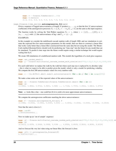
sage: v = finance.TimeSeries([1..10])
sage: v.vector()
(1.0, 2.0, 3.0, 4.0, 5.0, 6.0, 7.0, 8.0, 9.0, 10.0)
sage.finance.time_series.autoregressive_fit(acvs)
Given a sequence of lagged autocovariances of length M produce a 1 , . . . , a p so that the first M autocovariance
coefficients of the autoregressive processes X t = a 1 X t1 +· · ·+a p X t−p +Z t are the same as the input sequence.
The function works by solving the Yule-Walker equations Γa = γ, where γ = (γ(1), . . . , γ(M)), a =
(a 1 , . . . , a M ), with γ(i) the autocovariance of lag i and Γ ij = γ(i − j).
EXAMPLES:
In this example we consider the multifractal cascade random walk of length 1000, and use simulations to estimate
the expected first few autocovariance parameters for this model, then use them to construct a linear filter
that works vastly better than a linear filter constructed from the same data but not using this model. The Monte-
Carlo method illustrated below should work for predicting one “time step” into the future for any model that can
be simulated. To predict k time steps into the future would require using a similar technique but would require
scaling time by k.
We create 100 simulations of a multifractal random walk. This models the logarithms of a stock price sequence.
sage: set_random_seed(0)
sage: y = finance.multifractal_cascade_random_walk_simulation(3700,0.02,0.01,0.01,1000,100)
For each walk below we replace the walk by the walk but where each step size is replaced by its absolute value
– this is what we expect to be able to predict given the model, which is only a model for predicting volatility.
We compute the first 200 autocovariance values for every random walk:
sage: c = [[a.diffs().abs().sums().autocovariance(i) for a in y] for i in range(200)]
We make a time series out of the expected values of the autocovariances:
sage: ac = finance.TimeSeries([finance.TimeSeries(z).mean() for z in c])
sage: ac
[3.9962, 3.9842, 3.9722, 3.9601, 3.9481 ... 1.7144, 1.7033, 1.6922, 1.6812, 1.6701]
Note: ac looks like a line – one could best fit it to yield a lot more approximate autocovariances.
We compute the autoregression coefficients matching the above autocovariances:
sage: F = finance.autoregressive_fit(ac); F
[0.9982, -0.0002, -0.0002, 0.0003, 0.0001 ... 0.0002, -0.0002, -0.0000, -0.0002, -0.0014]
Note that the sum is close to 1:
sage: sum(F)
0.99593284089454...
Now we make up an ‘out of sample’ sequence:
sage: y2 = finance.multifractal_cascade_random_walk_simulation(3700,0.02,0.01,0.01,1000,1)[0].di
sage: y2
[0.0013, 0.0059, 0.0066, 0.0068, 0.0184 ... 6.8004, 6.8009, 6.8063, 6.8090, 6.8339]
And we forecast the very last value using our linear filter; the forecast is close:
sage: y2[:-1].autoregressive_forecast(F)
6.7836741372407...
20 Chapter 1. Time Series