Sage Reference Manual: Quantitative Finance - Mirrors

Sage Reference Manual: Quantitative Finance, Release 6.1.1
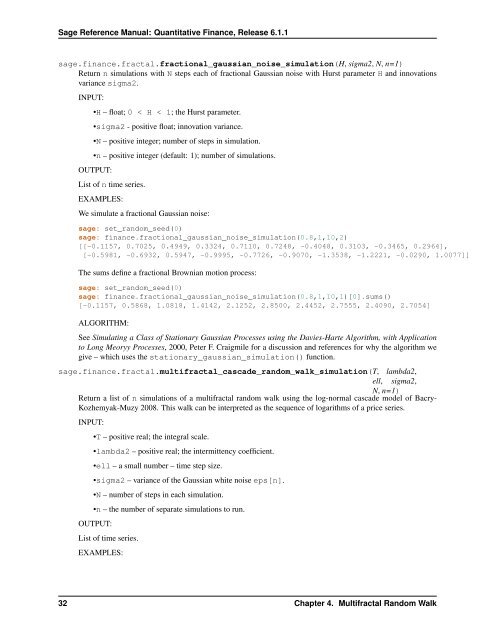
sage.finance.fractal.fractional_gaussian_noise_simulation(H, sigma2, N, n=1)
Return n simulations with N steps each of fractional Gaussian noise with Hurst parameter H and innovations
variance sigma2.
INPUT:
•H – float; 0 < H < 1; the Hurst parameter.
•sigma2 - positive float; innovation variance.
•N – positive integer; number of steps in simulation.
•n – positive integer (default: 1); number of simulations.
OUTPUT:
List of n time series.
EXAMPLES:
We simulate a fractional Gaussian noise:
sage: set_random_seed(0)
sage: finance.fractional_gaussian_noise_simulation(0.8,1,10,2)
[[-0.1157, 0.7025, 0.4949, 0.3324, 0.7110, 0.7248, -0.4048, 0.3103, -0.3465, 0.2964],
[-0.5981, -0.6932, 0.5947, -0.9995, -0.7726, -0.9070, -1.3538, -1.2221, -0.0290, 1.0077]]
The sums define a fractional Brownian motion process:
sage: set_random_seed(0)
sage: finance.fractional_gaussian_noise_simulation(0.8,1,10,1)[0].sums()
[-0.1157, 0.5868, 1.0818, 1.4142, 2.1252, 2.8500, 2.4452, 2.7555, 2.4090, 2.7054]
ALGORITHM:
See Simulating a Class of Stationary Gaussian Processes using the Davies-Harte Algorithm, with Application
to Long Meoryy Processes, 2000, Peter F. Craigmile for a discussion and references for why the algorithm we
give – which uses the stationary_gaussian_simulation() function.
sage.finance.fractal.multifractal_cascade_random_walk_simulation(T, lambda2,
ell, sigma2,
N, n=1)
Return a list of n simulations of a multifractal random walk using the log-normal cascade model of Bacry-
Kozhemyak-Muzy 2008. This walk can be interpreted as the sequence of logarithms of a price series.
INPUT:
•T – positive real; the integral scale.
•lambda2 – positive real; the intermittency coefficient.
•ell – a small number – time step size.
•sigma2 – variance of the Gaussian white noise eps[n].
•N – number of steps in each simulation.
•n – the number of separate simulations to run.
OUTPUT:
List of time series.
EXAMPLES:
32 Chapter 4. Multifractal Random Walk