English - Alps Know-How - Cipra

Report on the State of the Alps
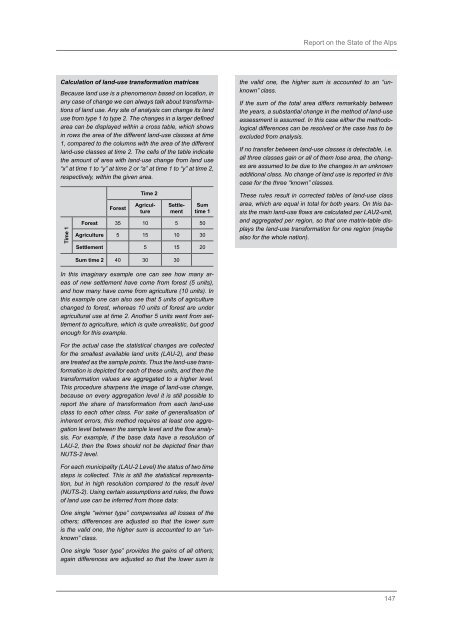
Calculation of land-use transformation matrices
Because land use is a phenomenon based on location, in
any case of change we can always talk about transformations
of land use. Any site of analysis can change its land
use from type 1 to type 2. The changes in a larger defined
area can be displayed within a cross table, which shows
in rows the area of the different land-use classes at time
1, compared to the columns with the area of the different
land-use classes at time 2. The cells of the table indicate
the amount of area with land-use change from land use
“x” at time 1 to “y” at time 2 or “a” at time 1 to “y” at time 2,
respectively, within the given area.
Time 1
Forest
Time 2
Agriculture
Settlement
Sum
time 1
Forest 35 10 5 50
Agriculture 5 15 10 30
Settlement 5 15 20
the valid one, the higher sum is accounted to an “unknown”
class.
If the sum of the total area differs remarkably between
the years, a substantial change in the method of land-use
assessment is assumed. In this case either the methodological
differences can be resolved or the case has to be
excluded from analysis.
If no transfer between land-use classes is detectable, i.e.
all three classes gain or all of them lose area, the changes
are assumed to be due to the changes in an unknown
additional class. No change of land use is reported in this
case for the three “known” classes.
These rules result in corrected tables of land-use class
area, which are equal in total for both years. On this basis
the main land-use flows are calculated per LAU2-unit,
and aggregated per region, so that one matrix-table displays
the land-use transformation for one region (maybe
also for the whole nation).
Sum time 2 40 30 30
In this imaginary example one can see how many areas
of new settlement have come from forest (5 units),
and how many have come from agriculture (10 units). In
this example one can also see that 5 units of agriculture
changed to forest, whereas 10 units of forest are under
agricultural use at time 2. Another 5 units went from settlement
to agriculture, which is quite unrealistic, but good
enough for this example.
For the actual case the statistical changes are collected
for the smallest available land units (LAU-2), and these
are treated as the sample points. Thus the land-use transformation
is depicted for each of these units, and then the
transformation values are aggregated to a higher level.
This procedure sharpens the image of land-use change,
because on every aggregation level it is still possible to
report the share of transformation from each land-use
class to each other class. For sake of generalisation of
inherent errors, this method requires at least one aggregation
level between the sample level and the flow analysis.
For example, if the base data have a resolution of
LAU-2, then the flows should not be depicted finer than
NUTS-2 level.
For each municipality (LAU-2 Level) the status of two time
steps is collected. This is still the statistical representation,
but in high resolution compared to the result level
(NUTS-2). Using certain assumptions and rules, the flows
of land use can be inferred from those data:
One single “winner type” compensates all losses of the
others; differences are adjusted so that the lower sum
is the valid one, the higher sum is accounted to an “unknown”
class.
One single “loser type” provides the gains of all others;
again differences are adjusted so that the lower sum is
147