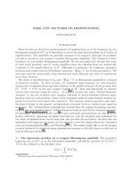
Park City Lectures on Eigenfunctions, Lecture 5: Lp norms of ...
Park City Lectures on Eigenfunctions, Lecture 5: Lp norms of ...
Park City Lectures on Eigenfunctions, Lecture 5: Lp norms of ...

Create successful ePaper yourself
Turn your PDF publications into a flip-book with our unique Google optimized e-Paper software.
<str<strong>on</strong>g>Park</str<strong>on</strong>g> <str<strong>on</strong>g>City</str<strong>on</strong>g> <str<strong>on</strong>g><strong>Lecture</strong>s</str<strong>on</strong>g> <strong>on</strong> Eigenfuncti<strong>on</strong>s, <strong>Lecture</strong> 5:<br />
L p <strong>norms</strong> <strong>of</strong> eigenfuncti<strong>on</strong>s<br />
July 20, 2013
Shapes and sizes <strong>of</strong> eigenfuncti<strong>on</strong>s<br />
This lecture is devoted to quantitative properties <strong>of</strong> L 2 normalized<br />
eigenfuncti<strong>on</strong>s <strong>of</strong> compact Riemannian manifolds (M, g). We<br />
measure the size <strong>of</strong> ϕ λ by the L p <strong>norms</strong>, ||ϕ λ || p .<br />
The main questi<strong>on</strong>s are:<br />
◮ How large can ||ϕ λ || p be, as (M, g) runs over all possible<br />
Riemannian manifolds and ϕ λ runs over all possible<br />
eigenfuncti<strong>on</strong>s <strong>of</strong> ∆ g ?<br />
◮ What types <strong>of</strong> eigenfuncti<strong>on</strong>s have extremal L p <strong>norms</strong>? Which<br />
(M, g) can have such eigenfuncti<strong>on</strong>s?<br />
◮ How do eigenfuncti<strong>on</strong>s c<strong>on</strong>centrate? Which <strong>on</strong>es are most<br />
c<strong>on</strong>centrated? How do eigenfuncti<strong>on</strong> c<strong>on</strong>centrati<strong>on</strong> reflect the<br />
global geometry <strong>of</strong> (M, g)?<br />
◮ We also broaden our focus to include quasi-modes or<br />
approximate eigenfuncti<strong>on</strong>s. They are <strong>of</strong>ten “semi-classical<br />
Lagrangian distributi<strong>on</strong>s”. We ask the same questi<strong>on</strong>s about<br />
them.
L p <strong>norms</strong><br />
We recall that<br />
∆ϕ λ = λ 2 ϕ λ ,<br />
∫<br />
M<br />
|ϕλ| 2 dV = 1.<br />
Let {ϕ j (x)} be an orth<strong>on</strong>ormal basis <strong>of</strong> eigenfuncti<strong>on</strong>s. To deal<br />
with possible multiplicities <strong>of</strong> eigenvalues, we c<strong>on</strong>sider the<br />
eigenspaces<br />
V λ = {ϕ : ∆ϕ = −λ 2 ϕ},<br />
and measure the growth rate <strong>of</strong> L p <strong>norms</strong> by<br />
We also c<strong>on</strong>sider<br />
L p (λ, g) =<br />
l p (λ, g) =<br />
sup ||ϕ|| L p. (1)<br />
ϕ∈V λ :||ϕ|| L 2 =1<br />
inf ||ϕ|| <strong>Lp</strong>. (2)<br />
ϕ∈V λ :||ϕ|| L 2 =1
Example: Irrati<strong>on</strong>al flat torus<br />
Let (M, g) be a flat irrati<strong>on</strong>al torus R n /L where L ⊂ R n is a<br />
co-compact lattice. In this case, the eigenfuncti<strong>on</strong>s are e i〈λ,x〉 with<br />
λ ∈ L ∗ .<br />
The multiplicities are 2 and it is easy to see that<br />
L p (λ, g) = l p (λ, g) = 1.<br />
How <strong>of</strong>ten do we find uniformly bounded eigenfuncti<strong>on</strong>s? Are there<br />
any examples besides the flat torus? (In fact no! if you restrict<br />
(M, g) to cases with integrable geodesic flow).
Sogge upper bounds <strong>on</strong> L p <strong>norms</strong> <strong>of</strong> eigenfuncti<strong>on</strong>s<br />
Theorem<br />
(Sogge, 1985)<br />
‖ϕ‖ p<br />
sup = O(λ δ(p) ), 2 ≤ p ≤ ∞ (3)<br />
ϕ∈V λ<br />
‖ϕ‖ 2<br />
where<br />
{<br />
n(<br />
1<br />
2<br />
δ(p) =<br />
− 1 p ) − 1 2 , 2(n+1)<br />
n−1<br />
≤ p ≤ ∞<br />
n−1<br />
2 ( 1 2 − 1 2(n+1)<br />
p<br />
), 2 ≤ p ≤<br />
n−1 . (4)
Dimensi<strong>on</strong> 2<br />
where<br />
‖ϕ‖ p<br />
sup = O(λ δ(p) ), 2 ≤ p ≤ ∞ (5)<br />
ϕ∈V λ<br />
‖ϕ‖ 2<br />
δ(p) =<br />
{<br />
2(<br />
1<br />
2 − 1 p ) − 1 2 = 1 2 − 2 p , 6 ≤ p ≤ ∞<br />
1<br />
2 ( 1 2 − 1 p ) = 1 4 − 1<br />
2p , 2 ≤ p ≤ 6. (6)<br />
The critical index is p = 6, and then δ(p) = 1 6 .
Extremals<br />
The upper bounds are sharp in the class <strong>of</strong> all (M, g) and are<br />
saturated <strong>on</strong> the round sphere:<br />
◮ For p > 2(n+1)<br />
n−1<br />
, z<strong>on</strong>al (rotati<strong>on</strong>ally invariant) spherical<br />
harm<strong>on</strong>ics saturate the L p bounds. Such eigenfuncti<strong>on</strong>s also<br />
occur <strong>on</strong> surfaces <strong>of</strong> revoluti<strong>on</strong>.<br />
◮ For L p for 2 ≤ p ≤ 2(n+1)<br />
n−1<br />
the bounds are saturated by highest<br />
weight spherical harm<strong>on</strong>ics, i.e. Gaussian beam al<strong>on</strong>g a stable<br />
elliptic geodesic. Such eigenfuncti<strong>on</strong>s also occur <strong>on</strong> surfaces<br />
<strong>of</strong> revoluti<strong>on</strong>.
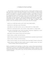
(i)Z<strong>on</strong>al eigenfuncti<strong>on</strong> (ii) Gaussian beam<br />
The left image is a z<strong>on</strong>al spherical harm<strong>on</strong>ic <strong>of</strong> degree N <strong>on</strong> S 2 : it<br />
has high peaks<strong>of</strong> height √ N at the north and south poles. The<br />
right image is a Gaussian beam: its height al<strong>on</strong>g the equator is<br />
N 1/4 and then it has Gaussian decay transverse to the equator.<br />
The z<strong>on</strong>al has high L p norm due to its high peaks <strong>on</strong> balls <strong>of</strong><br />
radius 1 N<br />
. The balls are so small that they do not have high <strong>Lp</strong><br />
<strong>norms</strong> for small p. The Gaussian beams are not as high but they<br />
are relatively high over an entire geodesic.
Spherical harm<strong>on</strong>ics <strong>of</strong> degree k<br />
Let H k ⊂ L 2 (S 2 ) denote the space <strong>of</strong> spherical harmn<strong>on</strong>ics <strong>of</strong><br />
degree k. Then:<br />
◮ L 2 (S n ) = ⊕ ∞<br />
k=0 H k. The sum is orthog<strong>on</strong>al.<br />
◮ Sp(∆ S n) = {λ k = k(k + 1)}.<br />
◮ dim H k = 2k + 1<br />
The group <strong>of</strong> rotati<strong>on</strong>s around the x 3 -axis commutes with the<br />
Laplacian. We denote its infinitesimal generator by L 3 = ∂<br />
i∂θ . We<br />
then c<strong>on</strong>sider the orth<strong>on</strong>ormal basis <strong>of</strong> joint eigenfuncti<strong>on</strong>s:<br />
⎧<br />
⎨ ∆ S 2Ym k = k(k + 1)Ym;<br />
k<br />
⎩<br />
∂<br />
i∂θ Y k m = mY k m.
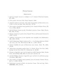
Oscillati<strong>on</strong> <strong>of</strong> a spherical harm<strong>on</strong>ic Y l m <strong>of</strong> low degree
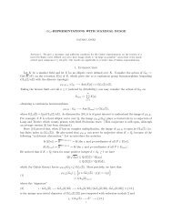
Oscillati<strong>on</strong> <strong>of</strong> a spherical harm<strong>on</strong>ic Y l m <strong>of</strong> high degree
Spectral projecti<strong>on</strong>s kernel = z<strong>on</strong>al harm<strong>on</strong>ic<br />
A key object in the theory <strong>of</strong> spherical harm<strong>on</strong>ics is the orthog<strong>on</strong>al<br />
projector<br />
Π k : L 2 (S 2 ) → H k .<br />
It has a kernel Π k (x, y) defined by<br />
∫<br />
Π k f (x) = Π k (x, y)f (y)dS(y).<br />
S n<br />
If {Y k m} is an orth<strong>on</strong>ormal basis <strong>of</strong> H k then<br />
d k<br />
∑<br />
Π k (x, y) = Ym(x)Y k m(y). k<br />
j=1
Coherent state Φ x k at x<br />
For each y, Π k (x, y) ∈ H k . We can L 2 normalize this functi<strong>on</strong> by<br />
dividing by the square root <strong>of</strong><br />
∫<br />
||Π k (·, y)|| 2 L<br />
= Π 2 k (x, y)Π k (y, x)dS(x) = Π k (x, x).<br />
S n<br />
We get<br />
Φ x k (y) = Π k(x, y)<br />
√<br />
Πk (x, x) .
Coherent states extremize L ∞ <strong>norms</strong><br />
This is simple and a standard fact about reproducing kernels. The<br />
‘coherent state’ obtained by pinning the spectral projecti<strong>on</strong>s kernel<br />
Π λ (x, y) for an eigenspace V λ at <strong>on</strong>e point y and dividing by its L 2<br />
norm is always the etremal for pointwise norm at y am<strong>on</strong>g<br />
eigenfuncti<strong>on</strong>s ϕ λ ∈ V λ<br />
∫<br />
ϕ λ (x) = Π λ (x, y)ϕ λ (y)dy<br />
M<br />
√ ∫<br />
=⇒ |ϕ λ (x)| ≤ |Π λ (x, y)| 2 dy = √ Π λ (x, x)<br />
M<br />
= |Φ x λ (x)|.<br />
In fact, they extremize L p <strong>norms</strong> for p ≥ p n
Normalized z<strong>on</strong>al harm<strong>on</strong>ics<br />
On S n , Π k (x, x) = C k since it is rotati<strong>on</strong>ally invariant and<br />
O(n + 1) acts transitively <strong>on</strong> S n . Its integral is dim H k , hence,<br />
Π k (x, x) = 1<br />
Vol(S n ) dim H k. Hence the normalized projecti<strong>on</strong> kernel<br />
with ‘peak’ at y 0 is<br />
Y k 0 (x) = Π k(x, y 0 ) √ Vol(S n )<br />
√ dim Hk<br />
.<br />
Here, we put y 0 equal to the north pole (0, 0 · · · , 1). The resulting<br />
functi<strong>on</strong> is called a z<strong>on</strong>al spherical harm<strong>on</strong>ic since it is invariant<br />
under the group O(n) <strong>of</strong> rotati<strong>on</strong>s fixing y 0 .
Highest weight spherical harm<strong>on</strong>ics = Gaussian beam<br />
Another important spherical harm<strong>on</strong>ic is Yk k , which is the spherical<br />
harm<strong>on</strong>ic in H k with the largest eigenvalue <strong>of</strong> L 3 = 1 ∂<br />
i ∂θ<br />
, or in<br />
other words the highest weight.<br />
It is an example <strong>of</strong> a Gaussian beam al<strong>on</strong>g a closed geodesic– a<br />
functi<strong>on</strong> like e iks e −ky 2<br />
in Fermi normal coordinates <strong>on</strong> the<br />
geodesic, with s arc-length and y the coordinate in the normal<br />
directi<strong>on</strong>. It is Gaussian in the normal directi<strong>on</strong>.<br />
Yk<br />
k is the restricti<strong>on</strong> <strong>of</strong> the harm<strong>on</strong>ic polynomial(x 1 + ix 2 ) k (up to<br />
normalizati<strong>on</strong>).
Gaussian Beam: maximizes L p <strong>norms</strong> for 2 ≤ p ≤ 6
Gaussian Beam 2: again, maximizes L p <strong>norms</strong> for<br />
2 ≤ p ≤ 6
Intuitive principle<br />
The fact that the z<strong>on</strong>al harm<strong>on</strong>ics and Gaussian beam are<br />
extremals for various L p <strong>norms</strong> is due the phase space geometry.<br />
They c<strong>on</strong>centrate <strong>on</strong> certain special kinds <strong>of</strong> invariant sets for the<br />
geodesic flow <strong>of</strong> S 2 . In general we expect:<br />
◮ Extremal eigenfuncti<strong>on</strong>s should c<strong>on</strong>centrate in phase space<br />
al<strong>on</strong>g special Lagrangian (or isotropic submanifolds) Λ ⊂ S ∗ M<br />
invariant under the geodesic flow.<br />
◮ Extremal eigenfuncti<strong>on</strong>s should be “semi-classical Lagrangian<br />
distributi<strong>on</strong>s”, i.e. quantum states corresp<strong>on</strong>ding to invariant<br />
Lagrangian submanifolds. They should be oscillatory integrals<br />
(WKB).<br />
◮ Their L p <strong>norms</strong> should reflect the singularity <strong>of</strong> the projecti<strong>on</strong><br />
π : Λ → M.
Lagrangian distributi<strong>on</strong>s<br />
Definiti<strong>on</strong>: A semi-classical Lagrangian distributi<strong>on</strong> <strong>on</strong> a manifold<br />
X is a sequence {u k (x)} <strong>of</strong> functi<strong>on</strong>s which may be represented as<br />
an oscillatory integral,<br />
u k (x) = −N/2<br />
k<br />
∫<br />
R N e i<br />
k<br />
ϕ(x,θ)<br />
a(x, θ, k )dθ.<br />
We assume that a(x, θ, ) is a semi-classical symbol,<br />
a(x, θ, ) ∼<br />
∞∑<br />
µ+k a k (x, θ).<br />
k=0<br />
It is assume that k → 0 as k → ∞.<br />
Often <strong>on</strong>e thinks <strong>of</strong> a c<strong>on</strong>tinuous parameter :<br />
u(x, ) = −N/2 ∫R N e i ϕ(x,θ) a(x, θ, )dθ.
Lagrangian distributi<strong>on</strong>s<br />
The Lagrangian distributi<strong>on</strong> is associated to the following<br />
Lagrangian submanifold <strong>of</strong> T ∗ X : Let<br />
Then c<strong>on</strong>sider<br />
C ϕ = {(x, θ) : d θ ϕ)x, θ) = 0}.<br />
ι ϕ (x, θ) = (x, d x ϕ(x, θ) : (x, θ) ∈ C ϕ }.<br />
Stati<strong>on</strong>ary phase methods show that u k (x) c<strong>on</strong>centrates <strong>on</strong> the<br />
Lagrangian submanifold Λ ϕ .<br />
The simplest examples are the exp<strong>on</strong>entials e i〈k,x〉 which<br />
c<strong>on</strong>centrates <strong>on</strong> the invariant torus ξ = k in<br />
T ∗ R n /Z n ≃ R n /Z n × R n .
Spherical harm<strong>on</strong>ic examples<br />
The normalized joint eigenfuncti<strong>on</strong>s <strong>on</strong> the standard sphere are<br />
given by<br />
√<br />
Ym N (N − m)!<br />
(θ, ϕ) = (2N + 1)<br />
(N + m)! PN m(cos ϕ)e imθ , (7)<br />
where<br />
P N m(cos ϕ) = 1<br />
2π<br />
∫ 2π<br />
are the Legendre polynomials.<br />
0<br />
(i sin ϕ cos θ + cos ϕ) N e −imθ dθ<br />
To obtain a Lagrangian distributi<strong>on</strong>, we c<strong>on</strong>sider a sequence <strong>of</strong> Y N m<br />
with m N → C for some C. I.e. we c<strong>on</strong>sider pairs k(m 0, N 0 ) lying <strong>on</strong><br />
a ray in the lattice in Z 2 <strong>of</strong> (m, N) with |m| ≤ N.
What is the Lagrangian submanifold?<br />
The Lagrangian submanifold <strong>of</strong> T ∗ S 2 associated to Y N m with<br />
m/N → c is the torus in S ∗ S 2 defined by<br />
p θ (x, ξ) := 〈ξ, ∂ ∂θ ) = c.<br />
This is a level set <strong>of</strong> the Clairaut integral<br />
p θ : S ∗ S 2 → [−1, 1].<br />
Examples: (i) The Lagrangian submanifold associated to the z<strong>on</strong>al<br />
spherical harm<strong>on</strong>ic is the “meridian torus” c<strong>on</strong>sisting <strong>of</strong> geodesics<br />
from the north to south poles.<br />
(ii) The Gaussian beam is associated to the unit vectors al<strong>on</strong>g the<br />
equator– a degenerate Lagrangian torus <strong>of</strong> dimensi<strong>on</strong> 1.
Should <strong>on</strong>e expect sequences <strong>of</strong> eigenfuncti<strong>on</strong>s to be<br />
Lagrangian distributi<strong>on</strong>s?<br />
NO!! It is very rare.<br />
It is true for joint eigenfuncti<strong>on</strong>s <strong>of</strong> commuting operators such as<br />
∂<br />
∂x j<br />
<strong>on</strong> R n /Z n ; or ∆ and L 3 = ∂ ∂θ (x 3 -axis rotati<strong>on</strong>s) for S 2 .<br />
These are quantum integrable Laplacians: ∆ commutes with n − 1<br />
other independent operators in dimensi<strong>on</strong> n. E.g ✷ for<br />
Schwarzchild spacetime.<br />
But these integrable systems are rare. Almost always,<br />
eigenfuncti<strong>on</strong>s are not at all like Lagrangian distributi<strong>on</strong>s. When<br />
the geodesic flow is ergodic they behave like “random waves”.
Intensity plot <strong>of</strong> an ergodic eigenfuncti<strong>on</strong> <strong>on</strong> an (ergodic)<br />
Bunimovich stadium: the mass is diffuse
(M, g) <strong>of</strong> maximal growth in L p <strong>norms</strong> <strong>of</strong> eigenfuncti<strong>on</strong>s<br />
We say that (M, g) has “maximal L p eigenfuncti<strong>on</strong> growth” if it<br />
possesses a sequence ϕ λjk <strong>of</strong> eigenfuncti<strong>on</strong>s which achieve the<br />
universal growth bounds.<br />
The standard S n has maximal eigenfuncti<strong>on</strong> growth. The flat torus<br />
does not. Nor do hyperbolic manifolds.<br />
How can <strong>on</strong>e characterize (M, g) <strong>of</strong> “maximal L p eigenfuncti<strong>on</strong><br />
growth” ?<br />
When does (M, g) possess a sequence <strong>of</strong> eigenfuncti<strong>on</strong>s achieving<br />
the maximal sup norm bound<br />
||ϕ λ || L ∞ ≤ Cλ n−1<br />
2 .
First c<strong>on</strong>diti<strong>on</strong> for maximal eigenfuncti<strong>on</strong> growth<br />
Theorem<br />
(Sogge-Z) If there exists a sequence {ϕ λjk } <strong>of</strong> eigenfuncti<strong>on</strong>s<br />
which achieves (saturates) the bound ||ϕ λ || L ∞ ≤ λ (n−1)/2 then<br />
there must exist a point x ∈ M for which the set<br />
L x = {ξ ∈ S ∗ x M : ∃T : exp x T ξ = x} (8)<br />
<strong>of</strong> directi<strong>on</strong>s <strong>of</strong> geodesic loops at x has positive surface measure.<br />
Here, exp is the exp<strong>on</strong>ential map, and the measure |Ω| <strong>of</strong> a set Ω<br />
is the <strong>on</strong>e induced by the metric g x <strong>on</strong> T ∗ x M. For instance, the<br />
poles x N , x S <strong>of</strong> a surface <strong>of</strong> revoluti<strong>on</strong> (S 2 , g) satisfy |L x | = 2π.
Is the loopset c<strong>on</strong>diti<strong>on</strong> sharp?<br />
No. There do exist (M, g) which possess ‘self focal points’ such<br />
that every geodesic emanating from the point returns to the point<br />
at the same time, yet the eigenfuncti<strong>on</strong> bounds are not achieved.<br />
Example: a tri-axial ellipsoid (three distinct axes, so not a surface<br />
<strong>of</strong> revoluti<strong>on</strong>). The umbilic points are self-focal points. However,<br />
the eigenfuncti<strong>on</strong>s which maximize the sup-norm <strong>on</strong>ly have L ∞<br />
<strong>norms</strong> <strong>of</strong> order λ n−1<br />
2 / log λ.
Special points and submanifolds<br />
◮ The z<strong>on</strong>al spherical harm<strong>on</strong>ics <strong>on</strong> S 2 or a surface <strong>of</strong> revoluti<strong>on</strong><br />
peak at the “poles”. We call a point p ∈ (M, g) a pole if all<br />
geodesics leaving p return to p at some fixed time T . These<br />
are the <strong>on</strong>ly known (to me) examples where the sup-norm<br />
bounds are achieved.<br />
◮ We also call a point p a self-focal point or blow-down point if<br />
all geodesics leaving p loop back to p at a comm<strong>on</strong> time T .<br />
They do not have to be closed geodesics. Examples: umbilic<br />
points <strong>of</strong> ellipsoids; foci <strong>of</strong> ellipses;<br />
◮ The <strong>on</strong>ly known examples <strong>of</strong> eigenfuncti<strong>on</strong>s saturating low L p<br />
bounds are Gaussian beams.
First return time and map<br />
Let T x : Sx ∗ M → R + ∪ {∞} denote the return time functi<strong>on</strong> to x,<br />
⎧<br />
⎨ inf{t > 0 : exp x tξ = x}, if ξ ∈ L x ;<br />
T x (ξ) =<br />
⎩<br />
+∞,<br />
if no such t exists.<br />
The first return map is define by<br />
Φ x := G Tx<br />
x : L x → S ∗ x M.<br />
It was first studied by Safarov et al to obtain a two-term local<br />
Weyl law when the set <strong>of</strong> loops at x has positive measure.
Additi<strong>on</strong>al necessary c<strong>on</strong>diti<strong>on</strong>s<br />
For simplicity we assume henceforth that (M, g) is real analytic.<br />
Then L x = S ∗ x M when |L x | > 0.<br />
At a self-focal point, with least comm<strong>on</strong> return time T x we define<br />
the first return map<br />
Φ x := G Tx : S ∗ x M → S ∗ x M.<br />
The additi<strong>on</strong>al necessary c<strong>on</strong>diti<strong>on</strong>, at least in the real analytic<br />
case, is that Φ x has no invariant L 2 functi<strong>on</strong>s.
Ellipsoid<br />
In the case <strong>of</strong> round S n , the first return map Φ x = Id for all x.<br />
Thus every directi<strong>on</strong> is recurrent.<br />
In the case <strong>of</strong> the triaxial ellipsoid satisfy, |R x | = 0 for each x ∈ M<br />
including the umbilic points wher |L x | = 1. The reas<strong>on</strong> is that Φ x<br />
at the umbilic points is a circle map with two fixed points<br />
corresp<strong>on</strong>ding to the two closed geodesics through x. One is<br />
stable, <strong>on</strong>e is unstable. Under iterati<strong>on</strong>s, Φ n x(ξ) tends to the stable<br />
fixed point for any ξ ∈ S ∗ x M except the unstable fixed point.<br />
Hence the <strong>on</strong>ly recurrent point is the stable fixed point.
Pole <strong>of</strong> a surface <strong>of</strong> revoluti<strong>on</strong> and umbilic points <strong>on</strong> an<br />
ellipsoid
New result<br />
Theorem<br />
(Z, Sogge 2013 +) If (M, g) is real analytic and has maximal<br />
eigenfuncti<strong>on</strong> growth, then it possesses a self-focal point whose<br />
first return map has an invariant functi<strong>on</strong> f ∈ L 2 (S ∗ x M, µ x ), where<br />
µ x is the Euclidean surface measure. Equivalently, it has an<br />
invariant measure |f | 2 dµ x which is absolutely c<strong>on</strong>tinuous with<br />
respect to dµ x
Sketch <strong>of</strong> pro<strong>of</strong><br />
◮ Suffices to show that R(λ, x) = o(λ m−1 ) uniformly in x ∈ M.<br />
Weyl remainder R(λ, x) can be expressed as an oscillatory<br />
integral over S ∗ x M à la Duistermaat-Guillemin, Safarov etc.<br />
◮ There <strong>on</strong>ly exist a finite number M T <strong>of</strong> self-focal points p<br />
with Φ p ≠ Id and first return time ≤ T <strong>on</strong> S ∗ pM in the real<br />
analytic case.<br />
◮ Ergodic theory shows that if Φ p has no L 2 -invariant functi<strong>on</strong>,<br />
then R(λ, p) = o(λ m−1 ). Thus, no invariant L 1 measures<br />
implies small remainders at self-focal points.<br />
◮ Oscillatory integral analysis shows that R(λ, x) = o(λ m−1 )<br />
uniformly if r(x, p) ≥ λ − 1 2 log λ for all self-focal points p.<br />
◮ Remaining step: R(λ, x) = o(λ m−1 ) uniformly if<br />
r(x, p) ≤ λ − 1 2 log λ assuming that R(λ, p) = o(λ m−1 ).
Heuristics<br />
We will study the remainder in the pointwise Weyl law rather than<br />
eigenfuncti<strong>on</strong>s per se. Since eigenfuncti<strong>on</strong>s are more intuitive, here<br />
is a heuristic guide to what we prove:<br />
◮ |ϕ j (x)| 2 can <strong>on</strong>ly achieve the maximum possible size at or<br />
very near a self-focal point.<br />
◮ If the first return map has no invariant L 1 measures at the<br />
self-focal point, then |ϕ j (x)| 2 cannot achieve the maximum<br />
possible size right at the self-focal point.<br />
◮ Using the smoothess <strong>of</strong> the remainder in Weyl’s law, we also<br />
prove that if it does not have the maximal order <strong>of</strong> magnitude<br />
at the self-focal point, then it cannot be maximally large very<br />
near it either.
Local Weyl law and L ∞ estimates <strong>of</strong> eigenfuncti<strong>on</strong>s<br />
E λ (x, x) = ∑ λ ν≤λ |ϕ ν(x)| 2<br />
with uniform remainder bounds<br />
= (2π) −n ∫ p(x,ξ)≤λ<br />
dξ + R(λ, x)<br />
|R(λ, x)| ≤ Cλ n−1 , x ∈ M.<br />
Since the integral in the local Weyl law is a c<strong>on</strong>tinuous functi<strong>on</strong> <strong>of</strong><br />
λ and since the spectrum <strong>of</strong> the Laplacian is discrete, this<br />
immediately gives<br />
∑<br />
|ϕ ν (x)| 2 ≤ 2Cλ n−1<br />
which in turn yields<br />
λ ν=λ<br />
<strong>on</strong> any compact Riemannian manifold.<br />
L ∞ (λ, g) = 0(λ n−1<br />
2 ) (9)
Local Weyl law with remainder<br />
The eigenfuncti<strong>on</strong> bounds are based <strong>on</strong> the following estimates for<br />
the local Weyl remainder.<br />
Theorem<br />
Let R(λ, x) denote the remainder for the local Weyl law at x. Then<br />
R(λ, x) = o(λ n−1 ) if |L x | = 0. (10)<br />
Additi<strong>on</strong>ally, if |L x | = 0 then, given ε > 0, there is a neighborhood<br />
N <strong>of</strong> x and a Λ =< ∞, both depending <strong>on</strong> ε so that<br />
|R(λ, y)| ≤ ελ n−1 , y ∈ N , λ ≥ Λ. (11)
Notati<strong>on</strong> for smoothed remainder<br />
Let ˆρ ∈ C0<br />
∞ be an even functi<strong>on</strong> with ˆρ(0) = 1, ρ(λ) > 0 for all<br />
λ ∈ R, and ˆρ T (t) = ˆρ( t T ).<br />
The classical cosine Tauberian method to determine Weyl<br />
asymptotics + remainder is to study<br />
ρ T ∗ dN(λ, x) = a 0 (x)λ n−1 + λ n−1 R(λ, x, T ), (12)<br />
where a 0 (x) is a smooth density ( = a c<strong>on</strong>stant C m in our case).<br />
We use large T ⇐⇒ l<strong>on</strong>g time behavior <strong>of</strong> the geodesic flow.
Oscillatory integral formula<br />
By the usual parametrix c<strong>on</strong>structi<strong>on</strong>: there exist phases ˜t j and<br />
amplitudes such that<br />
∫<br />
ρ T ∗ dN(λ, x) = ˆρ( t T )eiλt U(t, x, x)dt<br />
≃ λ n−1 ∑ j<br />
where the remainder is uniform in x.<br />
∫<br />
R<br />
S ∗ x M e iλ˜t j (x,ξ) ((ˆρ T a j0 )) |dξ| + O(λ n−2 ),<br />
Uses l<strong>on</strong>g time parametrix for U(t) = e it√∆ , polar coordinates in<br />
T ∗ M, and stati<strong>on</strong>ary phase in dtdr. ˜t j is the value <strong>of</strong> the phase<br />
ϕ j (t, x, x, ξ) at the critical point.
Many charts, many oscillatory integrals<br />
The index j runs over charts and local oscillatory integrals. Minor<br />
technical nuisance: we need to keep track <strong>of</strong> the number <strong>of</strong> charts<br />
as T grows; we w<strong>on</strong>’t emphasize this again. Then,<br />
∑<br />
∞<br />
ρ T ∗dN(λ, x) = a 0 λ n−1 +a 1 λ n−2 +λ n−1 R j (λ, x, T )+o T (λ n−1 ),<br />
with uniform remainder in x.<br />
j=1
Perr<strong>on</strong>-Frobenius operator<br />
Following Safarov, at a self-focal point x define<br />
U x : L 2 (Sx ∗ M, dµ x ) → L 2 (Sx ∗ M, dµ x ), U x f (ξ) := f (Φ x (ξ)) √ J x (ξ).<br />
(13)<br />
Here, J x is the Jacobian <strong>of</strong> the map Φ x , i.e. Φ ∗ x|dξ| = J x (ξ)|dξ|.<br />
Also define<br />
U x ± (λ) = e iλT ± x<br />
U x ± . (14)
Pointwise Weyl asymptotics: Safarov pre-trace formula<br />
If ˆρ = 0 in a neighborhood <strong>of</strong> t = 0 then<br />
ρ ′ ∗ N(λ, x) = λ ∑ ∫<br />
n−1 ˆρ(kT (ξ))U x (λ) k · 1dξ + o x (λ n−1 ).<br />
L x<br />
k∈Z\0<br />
Here, L x = {ξ ∈ S ∗ x M : exp x ξ = x} is the set <strong>of</strong> loops at x. Recall<br />
that<br />
U x f (ξ) = f (Φ x (ξ)) √ J Φ ,<br />
and that U x (λ)f = e iλ˜t(x,ξ) U x f .<br />
In the real analytic case, L x = S ∗ x M or has measure zero. In the<br />
latter case the integral is zero. The remainder is NON-UNIFORM<br />
in x, so we cannot use this directly and must study its pro<strong>of</strong>.
Decompositi<strong>on</strong> into almost loops and far from loops<br />
Pick f ≥ 0 ∈ C0<br />
∞ (R) which equals 1 <strong>on</strong> |s| ≤ 1 and zero for<br />
|s| ≥ 2 and split up the jth term into two terms using<br />
f (ɛ −2 |∇ ξ˜t j | 2 ) and 1 − f (ɛ −2 |∇ ξ˜t j | 2 ):<br />
where<br />
R j (λ, x, T ) = R j1 (λ, x, T ) + R j2 (λ, x, T ), (15)<br />
R j1 (λ, x; ɛ) := ∫ S ∗ x M eiλ˜t j<br />
f (ɛ −1 |∇ ξ˜t j (x, ξ)| 2 )(ˆρ(T x (ξ)))a 0 (T x (ξ), x, ξ)dξ<br />
(16)<br />
The sec<strong>on</strong>d term R j2 comes from the 1 − f (ɛ −2 |∇ ξ T x (ξ)| 2 ) term.<br />
Lemma<br />
For ɛ ≥ λ − 1 2 log λ we have<br />
sup |R 2 (λ, x, ɛ)| ≤ C(log λ) −1 .<br />
x∈M
Decompositi<strong>on</strong> <strong>of</strong> R 1 into loops and almost loops<br />
On the critical set where {∇ ξ˜t j (x, ξ) = 0} ⊂ S ∗ x M, we get<br />
∫<br />
L x<br />
e iλTx (ξ) ˆρ(T x (ξ))a 0 (T x , ξ), xξ)r n ∗ |dξ|. (17)<br />
We may decompose R j1 into<br />
∫<br />
R j1 (x, ɛ, T ) = e iλTx (ξ) ˆρ(T x (ξ))a 0 (T x , ξ), xξ)|dξ| + ˜R j1 , (18)<br />
L x<br />
where<br />
∫<br />
˜R j1 (x, ɛ, T ) =<br />
|∇˜t j |>0<br />
e iλ˜t(x,ξ) f (ɛ −2 |∇ ξ˜t j (x, ξ)| 2 )a 0 (T x (ξ), x, ξ)dξ.<br />
The integral over the loopset is the U x (λ) term above.<br />
(19)
Recap<br />
So far, for every x ∈ M, we decompose R(λ, x) into dynamical<br />
term <strong>on</strong> the loop set. It is zero if x is not self-focal point, and it is<br />
the whole integral if it is a self-focal point.<br />
If it is n<strong>on</strong> self-focal, we <strong>on</strong>ly get a n<strong>on</strong>-dynamical term ˜R j1 and<br />
another n<strong>on</strong>-dynamical term, R 2 which is small. We show that we<br />
can neglect the points outside <strong>of</strong> ⋃ M<br />
j=1 B δ(x j ) with δ = λ −1/2 log λ.<br />
We now c<strong>on</strong>sider the centers <strong>of</strong> the balls: i.e. self-focal points.
Ergodic theory at the self-focal points<br />
Here is the main result showing that R(λ, x) is small at the<br />
self-focal points if there do not exist invariant L 2 functi<strong>on</strong>s.<br />
Propositi<strong>on</strong><br />
Assume that U x has no invariant L 2 functi<strong>on</strong> for any x. Then, for<br />
all η > 0, there exists T independent <strong>of</strong> x so that for every<br />
self-focal point x,<br />
1<br />
T<br />
∫<br />
∣<br />
∞ ∑<br />
L x k=1<br />
ˆρ( T x<br />
(k)<br />
T<br />
(ξ)<br />
)Ux k · 1|dξ|<br />
≤ η. (20)<br />
∣
Real analyticity implies the number <strong>of</strong> self-focal points<br />
with twisted Φ x is finite<br />
Two key points:<br />
◮ As menti<strong>on</strong>ed above, in the real analytic case, there can <strong>on</strong>ly<br />
exist a finite number M(T ) <strong>of</strong> self-focal points with return<br />
time ≤ T if there are no points with Φ x = Id. Thus, the<br />
ergodic theory is uniform! But it <strong>on</strong>ly applies at self-focal<br />
points. This is the <strong>on</strong>ly place that we really use real<br />
analyticity.<br />
◮ Far from focal points, the measure <strong>of</strong> “almost critical points”<br />
(i.e. loops) is small and we can neglect these.
Uniform o(λ n−1 ) outside <strong>of</strong> small balls around self-focal<br />
points<br />
. We surround each by a ball B δ (x j ) with δ to be chosen later. In<br />
M\ ⋃ M<br />
j=1 B δ(x j ), there do not exist almost any critical directi<strong>on</strong>s<br />
nor almost critical directi<strong>on</strong>s. For sufficiently large T (the first<br />
return time) and for sufficiently small δ, the remainders R(λ, x) are<br />
uniformly small in this set. This just follows from the fact that<br />
there are almost no critical points.
Estimate near the self-focal points<br />
This reduces the problem to studying remainder estimates for<br />
points <strong>of</strong> ⋃ M<br />
j=1 B δ(x j ) − {x j }. We may let δ = λ − 1 2 log λ. We show<br />
that the remainder R(λ, x) at these points is bounded (up to<br />
c<strong>on</strong>stants independent <strong>of</strong> (x, λ)) by the remainder at the center<br />
the corresp<strong>on</strong>ding ball. The reas<strong>on</strong> is that the<br />
|R(x, λ, T ) − R(x j , λ, T )| ≤ Ce aT dist(x, x j ).<br />
Hence if the distance is O(λ −1/2 ) we may let T = α log λ to make<br />
this term small.<br />
The ergodic theorem is uniform for a finite set <strong>of</strong> points, so given<br />
ɛ, we may pick T (i.e. λ) large enough to make |R(x j , λ, T )| ≤ ɛ.
Summing up<br />
◮ No eigenfuncti<strong>on</strong> ϕ j (x) can be maximally large at a point x<br />
which is ≥ λ − 1 2<br />
j<br />
log λ j away from the self-focal points.<br />
◮ When there are no invariant measures, it also cannot be large<br />
at a self-focal point.<br />
◮ Using the jump <strong>of</strong> the remainder, we also see that if it is not<br />
large at a self-focal point, it cannot be maximally large very<br />
near it either.