Matlab code for damping identification using energy ... - CFD4Aircraft
Matlab code for damping identification using energy ... - CFD4Aircraft
Matlab code for damping identification using energy ... - CFD4Aircraft

Create successful ePaper yourself
Turn your PDF publications into a flip-book with our unique Google optimized e-Paper software.
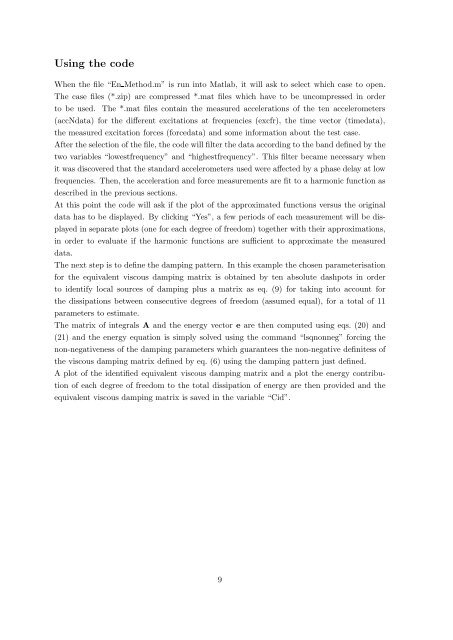
Using the <strong>code</strong><br />
When the file “En Method.m” is run into <strong>Matlab</strong>, it will ask to select which case to open.<br />
The case files (*.zip) are compressed *.mat files which have to be uncompressed in order<br />
to be used. The *.mat files contain the measured accelerations of the ten accelerometers<br />
(accNdata) <strong>for</strong> the different excitations at frequencies (excfr), the time vector (timedata),<br />
the measured excitation <strong>for</strong>ces (<strong>for</strong>cedata) and some in<strong>for</strong>mation about the test case.<br />
After the selection of the file, the <strong>code</strong> will filter the data according to the band defined by the<br />
two variables “lowestfrequency” and “highestfrequency”. This filter became necessary when<br />
it was discovered that the standard accelerometers used were affected by a phase delay at low<br />
frequencies. Then, the acceleration and <strong>for</strong>ce measurements are fit to a harmonic function as<br />
described in the previous sections.<br />
At this point the <strong>code</strong> will ask if the plot of the approximated functions versus the original<br />
data has to be displayed. By clicking “Yes”, a few periods of each measurement will be displayed<br />
in separate plots (one <strong>for</strong> each degree of freedom) together with their approximations,<br />
in order to evaluate if the harmonic functions are sufficient to approximate the measured<br />
data.<br />
The next step is to define the <strong>damping</strong> pattern. In this example the chosen parameterisation<br />
<strong>for</strong> the equivalent viscous <strong>damping</strong> matrix is obtained by ten absolute dashpots in order<br />
to identify local sources of <strong>damping</strong> plus a matrix as eq. (9) <strong>for</strong> taking into account <strong>for</strong><br />
the dissipations between consecutive degrees of freedom (assumed equal), <strong>for</strong> a total of 11<br />
parameters to estimate.<br />
The matrix of integrals A and the <strong>energy</strong> vector e are then computed <strong>using</strong> eqs. (20) and<br />
(21) and the <strong>energy</strong> equation is simply solved <strong>using</strong> the command “lsqnonneg” <strong>for</strong>cing the<br />
non-negativeness of the <strong>damping</strong> parameters which guarantees the non-negative definitess of<br />
the viscous <strong>damping</strong> matrix defined by eq. (6) <strong>using</strong> the <strong>damping</strong> pattern just defined.<br />
A plot of the identified equivalent viscous <strong>damping</strong> matrix and a plot the <strong>energy</strong> contribution<br />
of each degree of freedom to the total dissipation of <strong>energy</strong> are then provided and the<br />
equivalent viscous <strong>damping</strong> matrix is saved in the variable “Cid”.<br />
9