pdf version - Oomph-lib

Chapter 1 

Demo problem: Compression of 2D 

circular disk 

In this example we study the compression of a 2D circular disk, loaded by an external pressure. We also 

demonstrate: 

• how to "upgrade" a Mesh to a SolidMesh 

• why it is necessary to use "undeformed MacroElements" to ensure that the numerical results converge 

to the correct solution under mesh refinement if the domain has curvilinear boundaries. 

• how to switch between different constitutive equations 

• how to incorporate isotropic growth into the model 

We validate the numerical results by comparing them against the analytical solution of the equations of 

linear elasticity which are valid for small deflections. 

1.1 The problem 

The figure below shows a sketch of the basic problem: A 2D circular disk of radius a is loaded by a uniform 

pressure p ∗ 0. We wish to compute the disk’s deformation for a variety of constitutive equations.

2 Demo problem: Compression of 2D circular disk 

Figure 1.1: Sketch of the problem. 

The next sketch shows a variant of the problem: We assume that the material undergoes isotropic growth 

(e.g. via a biological growth process or thermal expension, say) with a constant growth factor Γ. We 

refer to the the document "Solid mechanics: Theory and implementation" for a detailed 

discussion of the theory of isotropic growth. Briefly, the growth factor defines the relative increase in the 

volume of an infinitesimal material element, relative to its volume in the stress-free reference configuration. 

If the growth factor is spatially uniform, isotropic growth leads to a uniform expansion √ of the material. 

For a circular disk, uniform growth increases the disk’s radius from a 0 to a = a 0 Γ without inducing 

any internal stresses. This uniformly expanded disk may then be regarded as the stress-free reference 

configuration upon which the external pressure acts. 

Figure 1.2: Sketch of the problem. 

Generated on Mon Aug 10 11:38:59 2009 by Doxygen

1.2 Results 3 

1.2 Results 

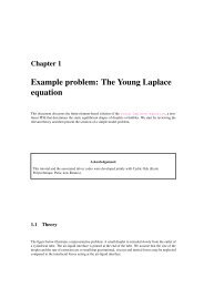
The animation shows the disk’s deformation when subjected to uniform growth of Γ = 1.1 and loaded by 

a pressure that ranges from negative to positive values. All lengths were scaled on the disks initial radius 

(i.e. its radius in the absence of growth and without any external load). 

Figure 1.3: Deformation of the uniformly grown disk when subjected to an external pressure. 

The figure below illustrates the disk’s load-displacement characteristics by plotting the disk’s nondimensional 

radius as function of the non-dimensional pressure, p 0 = p ∗ 0/S , where S is the characteristic 

stiffness of the material, for a variety of constitutive equations. 

Figure 1.4: Load displacement characteristics for various constitutive equations. 



1.2.1 Generalised Hooke’s law 

The blue, dash-dotted line corresponds to oomph-lib’s generalisation of Hooke’s law (with Young’s 

modulus E and Poisson ratio ν ) in which the dimensionless second Piola Kirchhoff stress tensor (nondimensionalised 

with the material’s Young’s modulus E, so that S = E ) is given by 

σ ij = 

1 

2(1 + ν) 

( 

G ik G jl + G il G jk + 

2ν ) 

1 − 2ν Gij G kl γ kl . 

Here γ ij = 1/2(G ij − g ij ) is Green’s strain tensor, formed from the difference between the deformed and 

undeformed metric tensors, G ij and g ij , respectively. The three different markers identify the results obtained 

with the two forms of the principle of virtual displacement, employing the displacement formulation 

(squares), and a pressure/displacement formulation with a continuous (delta) and a discontinuous (nabla) 

pressure interpolation. 

For zero pressure the disk’s non-dimensional radius is equal to the uniformly grown radius √ Γ = 1.0488. 

For small pressures the load-displacement curve follows the linear approximation 

r = √ Γ ( 1 − p 0 (1 + ν)(1 − 2ν) ) . 

We note that the generalised Hooke’s law leads to strain softening behaviour under compression (the pressure 

required to reduce the disk’s radius to a given value increases more rapidly than predicted by the linear 

approximation) whereas under expansion (for negative external pressures) the behaviour is strain softening. 

1.2.2 Generalised Mooney-Rivlin law 

The red, dashed line illustrates the behaviour when Fung & Tong’s generalisation of the Mooney-Rivlin law 

(with Young’s modulus, E, Poisson ratio ν and Mooney-Rivlin parameter C 1 ) is used as the constitutive 

equation. For this constitutive law, the non-dimensional strain energy function W = W ∗ /S, where the 

characteristic stress is given by Young’s modulus, i.e. S = E, is given by 

where 

W = 1 2 (I 2 G(1 − ν) 

1 − 3) + (G − C 1 )(I 2 − 3) + (C 1 − 2G)(I 3 − 1) + (I 3 − 1) 

2(1 − 2ν) , 

G = 

E 

2(1 + ν) 

is the shear modulus, and I 1 , I 2 and I 3 are the three invariants of Green’s strain tensor. See "Solid 

mechanics: Theory and implementation" for a detailed discussion of strain energy functions. 

The figure shows that for small deflections, the disk’s behaviour is again well approximated by 

linear elasticity. However, in the large-displacement regime the Mooney-Rivlin is strain hardening under 

extension and softening under compression when compared to the linear elastic behaviour. 

1.3 Global parameters and functions 

As usual we define the global problem parameters in a namespace. We provide pointers to the constitutive 

equations and strain energy functions to be explored, and define the associated constitutive parameters. 

//============namespace_for_problem_parameters===================== 

/// Global variables 

//================================================================= 

namespace Global_Physical_Variables 

{ 

/// Pointer to strain energy function 


1.4 The driver code 5 

StrainEnergyFunction* Strain_energy_function_pt; 

/// Pointer to constitutive law 

ConstitutiveLaw* Constitutive_law_pt; 

/// Elastic modulus 

double E=1.0; 

/// Poisson’s ratio 

double Nu=0.3; 

/// "Mooney Rivlin" coefficient for generalised Mooney Rivlin law 

double C1=1.3; 

Next we define the pressure load, using the general interface defined in the SolidTractionElement 

class. The arguments of the function reflect that the load on a solid may be a function of the Lagrangian 

and Eulerian coordinates, and the external unit normal on the solid. Here we apply a spatially constant 

external pressure of magnitude P which acts in the direction of the negative outer unit normal on the solid. 

/// Uniform pressure 

double P = 0.0; 

/// Constant pressure load 

void constant_pressure(const Vector &xi,const Vector &x, 

const Vector &n, Vector &traction) 

{ 

unsigned dim = traction.size(); 

for(unsigned i=0;i


{ 

// Store command line arguments 

CommandLineArgs::setup(argc,argv); 

// Define a strain energy function: Generalised Mooney Rivlin 

Global_Physical_Variables::Strain_energy_function_pt = 

new GeneralisedMooneyRivlin(&Global_Physical_Variables::Nu, 

&Global_Physical_Variables::C1, 

&Global_Physical_Variables::E); 

// Define a constitutive law (based on strain energy function) 

Global_Physical_Variables::Constitutive_law_pt = 

new IsotropicStrainEnergyFunctionConstitutiveLaw( 

Global_Physical_Variables::Strain_energy_function_pt); 

We build a problem object, using the displacement-based RefineableQPVDElements to discretise the 

domain, and perform a parameter study, exploring the disk’s deformation for a range of external pressures. 

// Case 0: No pressure, generalised Mooney Rivlin 

//----------------------------------------------- 

{ 

//Set up the problem 

StaticDiskCompressionProblem problem; 

cout

1.4 The driver code 7 

StaticDiskCompressionProblem 

problem; 

cout


} // done case 5 

// Clean up 

delete Global_Physical_Variables::Constitutive_law_pt; 

Global_Physical_Variables::Constitutive_law_pt=0; 

} // end of main 

1.5 The mesh 

We formulate the problem in cartesian coordinates (ignoring the problem’s axisymmetry) but discretise 

only one quarter of the domain, applying appropriate symmetry conditions along the x and y axes. The 

computational domain may be discretised with the RefineableQuarterCircleSectorMesh that 

we already used in many previous examples. To use the mesh in this solid mechanics problem we must 

first "upgrade" it to a SolidMesh. This is easily done by multiple inheritance: 

//==========start_mesh================================================= 

/// Elastic quarter circle sector mesh with functionality to 

/// attach traction elements to the curved surface. We "upgrade" 

/// the RefineableQuarterCircleSectorMesh to become an 

/// SolidMesh and equate the Eulerian and Lagrangian coordinates, 

/// thus making the domain represented by the mesh the stress-free 

/// configuration. 

/// \n\n 

/// The member function \c make_traction_element_mesh() creates 

/// a separate mesh of SolidTractionElements that are attached to the 

/// mesh’s curved boundary (boundary 1). 

//===================================================================== 

template 

class ElasticRefineableQuarterCircleSectorMesh : 

public virtual RefineableQuarterCircleSectorMesh, 

public virtual SolidMesh 

{ 

The constructor calls the constructor of the underlying RefineableQuarterCircleSectorMesh 

and sets the Lagrangian coordinates of the nodes to their current Eulerian positions, making the initial 

configuration stress-free. 

public: 

/// \short Constructor: Build mesh and copy Eulerian coords to Lagrangian 

/// ones so that the initial configuration is the stress-free one. 

ElasticRefineableQuarterCircleSectorMesh(GeomObject* wall_pt, 

const double& xi_lo, 

const double& fract_mid, 

const double& xi_hi, 

TimeStepper* time_stepper_pt= 

&Mesh::Default_TimeStepper) : 

RefineableQuarterCircleSectorMesh(wall_pt,xi_lo,fract_mid,xi_hi, 

time_stepper_pt) 

{ 

/// Make the current configuration the undeformed one by 

/// setting the nodal Lagrangian coordinates to their current 

/// Eulerian ones 

set_lagrangian_nodal_coordinates(); 

} 

We also provide a helper function that creates a mesh of SolidTractionElements which are attached 

to the curved domain boundary (boundary 1). These elements will be used to apply the external pressure 

load. 


1.6 The Problem class 9 

/// Function to create mesh made of traction elements 

void make_traction_element_mesh(SolidMesh*& traction_mesh_pt) 

{ 

}; 

} 

// Make new mesh 

traction_mesh_pt = new SolidMesh; 

// Loop over all elements on boundary 1: 

unsigned b=1; 

unsigned n_element = this->nboundary_element(b); 

for (unsigned e=0;eboundary_element_pt(b,e); 

// Find the index of the face of element e along boundary b 

int face_index = this->face_index_at_boundary(b,e); 

// Create new element 

traction_mesh_pt->add_element_pt(new SolidTractionElement 

(fe_pt,face_index)); 

} 

1.6 The Problem class 

The definition of the Problem class is very straightforward. In addition to the constructor and the (empty) 

actions_before_newton_solve() and actions_after_newton_solve() functions, we 

provide the function parameter_study(...) which performs a parameter study, computing the disk’s 

deformation for a range of external pressures. The member data includes pointers to the mesh of "bulk" 

solid elements, and the mesh of SolidTractionElements that apply the pressure load. The trace file 

is used to document the disk’s load-displacement characteristics by plotting the radial displacement of the 

nodes on the curvlinear boundary, pointers to which are stored in the vector Trace_node_pt. 

//====================================================================== 

/// Uniform compression of a circular disk in a state of plane strain, 

/// subject to uniform growth. 

//====================================================================== 

template 

class StaticDiskCompressionProblem : public Problem 

{ 

public: 

/// Constructor: 

StaticDiskCompressionProblem(); 

/// Run simulation: Pass case number to label output files 

void parameter_study(const unsigned& case_number); 

/// Doc the solution 

void doc_solution(DocInfo& doc_info); 

/// Update function (empty) 

void actions_after_newton_solve() {} 

/// Update function (empty) 

void actions_before_newton_solve() {} 



private: 

/// Trace file 

ofstream Trace_file; 

/// Vector of pointers to nodes whose position we’re tracing 

Vector Trace_node_pt; 

/// Pointer to solid mesh 

ElasticRefineableQuarterCircleSectorMesh* Solid_mesh_pt; 

/// Pointer to mesh of traction elements 

SolidMesh* Traction_mesh_pt; 

}; 

1.7 The Constructor 

We start by constructing the mesh of "bulk" SolidElements, using the Ellipse object to specify the 

shape of the curvilinear domain boundary. 

//====================================================================== 

/// Constructor: 

//====================================================================== 

template 

StaticDiskCompressionProblem::StaticDiskCompressionProblem() 

{ 

// Build the geometric object that describes the curvilinear 

// boundary of the quarter circle domain 

Ellipse* curved_boundary_pt = new Ellipse(1.0,1.0); 

// The curved boundary of the mesh is defined by the geometric object 

// What follows are the start and end coordinates on the geometric object: 

double xi_lo=0.0; 

double xi_hi=2.0*atan(1.0); 

// Fraction along geometric object at which the radial dividing line 

// is placed 

double fract_mid=0.5; 

//Now create the mesh using the geometric object 

Solid_mesh_pt = new ElasticRefineableQuarterCircleSectorMesh( 

curved_boundary_pt,xi_lo,fract_mid,xi_hi); 

Next we choose the nodes on the curvilinear domain boundary (boundary 1) as the nodes whose displacement 

we document in the trace file. 

// Setup trace nodes as the nodes on boundary 1 (=curved boundary) 

// in the original mesh. 

unsigned n_boundary_node = Solid_mesh_pt->nboundary_node(1); 

Trace_node_pt.resize(n_boundary_node); 

for(unsigned j=0;jboundary_node_pt(1,j);} 

The QuarterCircleSectorMesh that forms the basis of the "bulk" mesh contains only three elements 

– not enough to expect the solution to be accurate. Therefore we apply one round of uniform 

mesh refinement before attaching the SolidTractionElements to the mesh boundary 1, using the 

function make_traction_element_mesh() in the ElasticRefineableQuarterCircle- 

SectorMesh. 


1.7 The Constructor 11 

// Refine the mesh uniformly 

Solid_mesh_pt->refine_uniformly(); 

// Now construct the traction element mesh 

Solid_mesh_pt->make_traction_element_mesh(Traction_mesh_pt); 

We add both meshes to the Problem and build a combined global mesh: 

// Solid mesh is first sub-mesh 

add_sub_mesh(Solid_mesh_pt); 

// Traction mesh is second sub-mesh 

add_sub_mesh(Traction_mesh_pt); 

// Build combined "global" mesh 

build_global_mesh(); 

Symmetry boundary conditions along the horizontal and vertical symmetry lines require that the nodes’ 

vertical position is pinned along boundary 0, while their horizontal position is pinned along boundary 2. 

// Pin the left edge in the horizontal direction 

unsigned n_side = mesh_pt()->nboundary_node(2); 

for(unsigned i=0;iboundary_node_pt(2,i)->pin_position(0);} 

// Pin the bottom in the vertical direction 

unsigned n_bottom = mesh_pt()->nboundary_node(0); 

for(unsigned i=0;iboundary_node_pt(0,i)->pin_position(1);} 

Since we are using refineable solid elements, we pin any "redundant" pressure degrees of freedom in the 

"bulk" solid mesh (see the exercises in another tutorial for a more detailed discussion of 

this issue). 

// Pin the redundant solid pressures (if any) 

PVDEquationsBase::pin_redundant_nodal_solid_pressures( 

Solid_mesh_pt->element_pt()); 

Next, we complete the build of the elements in the "bulk" solid mesh by passing the pointer to the constitutive 

equation and the pointer to the isotropic-growth function to the elements: 

//Complete the build process for elements in "bulk" solid mesh 

unsigned n_element =Solid_mesh_pt->nelement(); 

for(unsigned i=0;ielement_pt(i)); 

// Set the constitutive law 

el_pt->constitutive_law_pt() = 

Global_Physical_Variables::Constitutive_law_pt; 

// Set the isotropic growth function pointer 

el_pt->isotropic_growth_fct_pt()=Global_Physical_Variables::growth_function; 

} 

We repeat this exercise for the SolidTractionElements which must be given a pointer to the function 

that applies the pressure load 



// Complete build process for SolidTractionElements 

n_element=Traction_mesh_pt->nelement(); 

for(unsigned i=0;ielement_pt(i)); 

//Set the traction function 

el_pt->traction_fct_pt() = Global_Physical_Variables::constant_pressure; 

} 

Finally, we set up the equation numbering scheme and report the number of unknowns. 

//Set up equation numbering scheme 

cout size();} 

// Exact outer radius for linear elasticity 

double nu=Global_Physical_Variables::Nu; 

double exact_r=sqrt(Global_Physical_Variables::Uniform_gamma)* 

(1.0-Global_Physical_Variables::P/Global_Physical_Variables::E 

*((1.0+nu)*(1.0-2.0*nu))); 


1.9 Performing the parameter study 13 

// Write trace file: Problem parameters 

Trace_file


for(unsigned i=0;i

pdf version - Oomph-lib

Create successful ePaper yourself

Delete template?

Save as template?