Demo problem: Turek & Hron's FSI benchmark problem - Oomph-lib

Chapter 1 

Demo problem: Turek & Hron’s FSI 

benchmark problem 

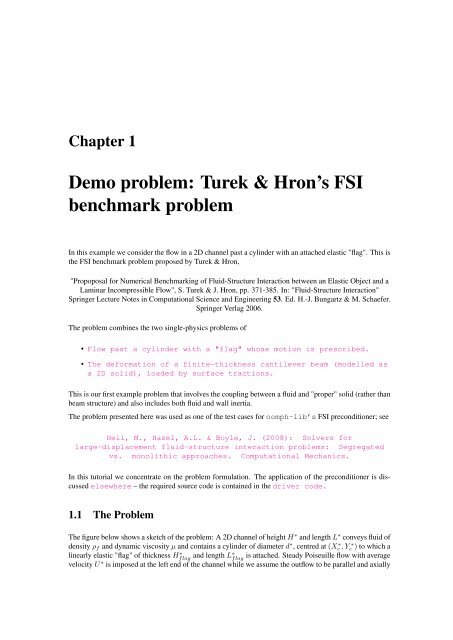
In this example we consider the flow in a 2D channel past a cylinder with an attached elastic "flag". This is 

the FSI benchmark problem proposed by Turek & Hron, 

"Propoposal for Numerical Benchmarking of Fluid-Structure Interaction between an Elastic Object and a 

Laminar Incompressible Flow", S. Turek & J. Hron, pp. 371-385. In: "Fluid-Structure Interaction" 

Springer Lecture Notes in Computational Science and Engineering 53. Ed. H.-J. Bungartz & M. Schaefer. 

Springer Verlag 2006. 

The problem combines the two single-physics problems of 

• Flow past a cylinder with a "flag" whose motion is prescribed. 

• The deformation of a finite-thickness cantilever beam (modelled as 

a 2D solid), loaded by surface tractions. 

This is our first example problem that involves the coupling between a fluid and "proper" solid (rather than 

beam structure) and also includes both fluid and wall inertia. 

The problem presented here was used as one of the test cases for oomph-lib’s FSI preconditioner; see 

Heil, M., Hazel, A.L. & Boyle, J. (2008): Solvers for 

large-displacement fluid-structure interaction problems: Segregated 

vs. monolithic approaches. Computational Mechanics. 

In this tutorial we concentrate on the problem formulation. The application of the preconditioner is discussed 

elsewhere – the required source code is contained in the driver code. 

1.1 The Problem 

The figure below shows a sketch of the problem: A 2D channel of height H ∗ and length L ∗ conveys fluid of 

density ρ f and dynamic viscosity µ and contains a cylinder of diameter d ∗ , centred at (Xc ∗ , Yc ∗ ) to which a 

linearly elastic "flag" of thickness Hflag ∗ and length L∗ flag 

is attached. Steady Poiseuille flow with average 

velocity U ∗ is imposed at the left end of the channel while we assume the outflow to be parallel and axially

2 Demo problem: Turek & Hron’s FSI benchmark problem 

traction-free. We model the flag as a linearly elastic Hookean solid with elastic modulus E ∗ , density ρ s 

and Poisson’s ratio ν. 

Figure 1.1: Sketch of the problem in dimensional variables. 

We non-dimensionalise all length and coordinates on the diameter of the cylinder, d ∗ , the velocities on 

the mean velocity, U ∗ , and the fluid pressure on the viscous scale. To faciliate comparisons with Turek 

& Hron’s dimensional benchmark data (particularly for the period of the self-excited oscillations), we 

use a timescale of T ∗ = 1 sec to non-dimensionalise time. The fluid flow is then governed by the nondimensional 

Navier-Stokes equations 

( 

Re St ∂u ) 

i 

∂t + u ∂u i 

j = − ∂p + 

∂ [( ∂ui 

+ ∂u )] 

j 

, 

∂x j ∂x i ∂x j ∂x j ∂x i 

where Re = ρU ∗ H ∗ 0 /µ and St = d ∗ /(U ∗ T ∗ ), and 

subject to parabolic inflow 

∂u i 

∂x i 

= 0, 

u = 6x 2 (1 − x 2 )e 1 

at the inflow cross-section; parallel, axially-traction-free outflow at the outlet; and no-slip on the stationary 

channel walls and the surface of the cylinder, u = 0. The no-slip condition on the moving flag is 

u = St ∂R w(ξ [top,tip,bottom] , t) 

∂t 

(1) 

where ξ [top,tip,bottom] are Lagrangian coordinates parametrising the three faces of the flag. 

We describe the deformation of the elastic flag by the non-dimensional position vector R(ξ 1 , ξ 2 , t) which 

is determined by the principle of virtual displacements 

∫ { ( ) } ∮ 

σ ij δγ ij − f − Λ 2 ∂2 R 

∂t 2 · δR dv − t · δR dA = 0, (2) 

A tract 

v 

where all solid stresses and tractions have been non-dimensionalised on Young’s modulus, E ∗ ; see the 

Solid Mechanics Tutorial for details. The solid mechanics timescale ratio (the ratio of the 

Generated on Mon Aug 10 11:44:25 2009 by Doxygen

1.2 Parameter values for the benchmark problems 3 

timescale T ∗ chosen to non-dimensionalise time, to the intrinsic timescale of the solid) can be expressed 

in terms of the Reynolds and Strouhal numbers, the density ratio, and the FSI interaction parameter as 

( √ ) d 

Λ 2 ∗ 

2 ( ) 

ρs 

= 

T ∗ E ∗ = St 2 ρs 

Re Q. 

ρ f 

Here is a sketch of the non-dimensional version of the problem: 

Figure 1.2: Sketch of the fluid problem in dimensionless variables, showing the Lagrangian coordinates 

that parametrise the three faces of the flag. 

1.2 Parameter values for the benchmark problems 

The (dimensional) parameter values given in Turek & Hron’s benchmark correspond to the following nondimensional 

parameters: 

1.2.1 Geometry 

• Cylinder diameter d = 1 

• Centre of cylinder X c = Y c = 2 

• Channel length L = 25 

• Channel width H = 4.1 

• Thickness of the undeformed flag H flag = 0.2 

• Right end of undeformed flag x tip = 6 

1.2.2 Non-dimensional parameters 

The three FSI test cases correspond to the following non-dimensional parameters: 

Re = 

U ∗ d ∗ ρ f /µ 

St = 

d ∗ /(U ∗ T ∗ ) 

Q = 

µU ∗ /(E ∗ d ∗ ) 

ρ s /ρ f Λ 2 = 

(d ∗ /T ∗√ ρ s /E ∗ ) 2 = 

St 2 (ρ s /ρ f )Re Q 

FSI1 20 0.5 1.429 × 10 −6 1 7.145 × 10 −6 





1.3 Results 

The test cases FSI2 and FSI3 are the most interesting because the system develops large-amplitude selfexcited 

oscillations 

1.3.1 FSI2 

Following an initial transient period the system settles into large-amplitude self-excited oscillations during 

which the oscillating flag generates a regular vortex pattern that is advected along the channel. This is 

illustrated in the figure below which shows a snapshot of the flow field (pressure contours and instantaneous 

streamlines) at t = 6.04. 

Figure 1.3: Snapshot of the flow field (instantaenous streamlines and pressure contours) 

The constantly adapted mesh contains and average of 65,000 degrees of freedom. A relatively large 

timestep of ∆t = 0.01 – corresponding to about 50 timesteps per period of the oscillation – was used 

in this computation. With this discretisation the system settles into oscillations with a period of ≈ 0.52 and 

an amplitude of the tip-displacement of 0.01 ± 0.83. 

Figure 1.4: Time trace of the tip displacement. 

1.3.2 FSI3 

The figures below shows the corresponding results for the case FSI3 in which the fluid and solid densities 

are equal and the Reynolds number twice as large as in the FSI2 case. The system performs oscillations 

of much higher frequency and smaller amplitude. This is illustrated in the figure below which shows a 

snapshot of the flow field (pressure contours and instantaneous streamlines) at t = 3.615. 


1.4 Overview of the driver code 5 

Figure 1.5: Snapshot of the flow field (instantaenous streamlines and pressure contours) 

This computation was performed with a timestep of ∆t = 0.005 and resulted in oscillations with a period 

of ≈ 0.19 and an amplitude of the tip-displacement of 0.01 ± 0.36. 

The increase in frequency and Reynolds number leads to the development of thinner boundary and shear 

layers which require a finer spatial resolution, involving an average of 84,000 degrees of freedom. 

Figure 1.6: Time trace of the tip displacement. 

1.4 Overview of the driver code 

Since the driver code is somewhat lengthy we start by providing a brief overview of the main steps in the 

Problem construction: 

1. We start by discretising the flag with 2D solid elements, as in the corresponding single-physics 

solid mechanics example. 

2. Next we attach FSISolidTractionElements to the three solid mesh boundaries that are exposed 

to the fluid traction. These elements are used to compute and impose the fluid traction onto 

the solid elements, using the flow field from the adjacent fluid elements. 

3. We now combine the three sets of FSISolidTractionElements into three individual (sub- 

)meshes and convert these to GeomObjects, using the MeshAsGeomObject class. 

4. The GeomObject representation of the three surface meshes is then passed to the constructor of the 

fluid mesh. The algebraic node-update methodology provided in the Algebraic- 

Mesh base class is used to update its nodal positions in response to the motion of its bounding 

GeomObjects. 

5. Finally, we use the helper function FSI_functions::setup_fluid_load_info_for_- 

solid_elements(...) to set up the fluid-structure interaction – this function determines which 

fluid elements are adjacent to the Gauss points in the FSISolidTractionElements that apply 

the fluid traction to the solid. 

6. Done! 



1.5 Parameter values for the benchmark problems 

As usual, We use a namespace to define the (many) global parameters, using default assignments for the 

FSI1 test case. 

//=====start_of_global_parameters================================= 

/// Global variables 

//================================================================ 

namespace Global_Parameters 

{ 

/// Default case ID 

string Case_ID="FSI1"; 

/// Reynolds number (default assignment for FSI1 test case) 

double Re=20.0; 

/// Strouhal number (default assignment for FSI1 test case) 

double St=0.5; 

/// \short Product of Reynolds and Strouhal numbers (default 

/// assignment for FSI1 test case) 

double ReSt=10.0; 

/// FSI parameter (default assignment for FSI1 test case) 

double Q=1.429e-6; 

/// \short Density ratio (solid to fluid; default assignment for FSI1 

/// test case) 

double Density_ratio=1.0; 

/// Height of flag 

double H=0.2; 

/// x position of centre of cylinder 

double Centre_x=2.0; 

/// y position of centre of cylinder 

double Centre_y=2.0; 

/// Radius of cylinder 

double Radius=0.5; 

/// Pointer to constitutive law 

ConstitutiveLaw* Constitutive_law_pt=0; 

/// \short Timescale ratio for solid (dependent parameter 

/// assigned in set_parameters()) 

double Lambda_sq=0.0; 

/// Timestep 

double Dt=0.1; 

/// Ignore fluid (default assignment for FSI1 test case) 

bool Ignore_fluid_loading=false; 

/// Elastic modulus 

double E=1.0; 

/// Poisson’s ratio 

double Nu=0.4; 

We also include a gravitational body force for the solid. (This is only used for the solid mechanics test 

cases, CSM1 and CSM2, which will not be discussed here.) 


1.5 Parameter values for the benchmark problems 7 

/// Non-dim gravity (default assignment for FSI1 test case) 

double Gravity=0.0; 

/// Non-dimensional gravity as body force 

void gravity(const double& time, 

const Vector &xi, 

Vector &b) 

{ 

b[0]=0.0; 

b[1]=-Gravity; 

} 

The domain geometry and flow field are fairly complex and it is difficult to construct a good initial guess 

for the Newton iteration. To ensure its convergence at the beginning of the simulation we therefore employ 

the method suggested by Turek & Hron: We start the flow from rest and ramp up the inflow profile from 

zero to its maximum value. The parameters for the time-dependent increase in the influx are defined here: 

/// Period for ramping up in flux 

double Ramp_period=2.0; 

/// Min. flux 

double Min_flux=0.0; 

/// Max. flux 

double Max_flux=1.0; 

/// \short Flux increases between Min_flux and Max_flux over 

/// period Ramp_period 

double flux(const double& t) 

{ 

if (t


} 

// FSI parameter 

Q=1.429e-6; 

// Timestep -- aiming for about 40 steps per period 

Dt=0.1; 

// Density ratio 

Density_ratio=1.0; 

// Gravity 

Gravity=0.0; 

// Max. flux 

Max_flux=1.0; 

// Ignore fluid 

Ignore_fluid_loading=false; 

// Compute dependent parameters 

// Timescale ratio for solid 

Lambda_sq=Re*Q*Density_ratio*St*St; 

In the interest of brevity we omit the listings of the assignments for the other cases. Finally, we select the 

length of the time interval over which the influx is ramped up from zero to its maximum value to be equal 

to 20 timesteps, create a constitutive equation for the solid, and document the parameter values used in the 

simulation: 

// Ramp period (20 timesteps) 

Ramp_period=Dt*20.0; 

// "Big G" Linear constitutive equations: 

Constitutive_law_pt = new GeneralisedHookean(&Nu,&E); 

// Doc 

oomph_info

1.6 The driver code 9 

interpreted as the code being run as part of oomph-lib’s self-test procedure in which case we perform 

a computation with the parameter values for case FSI1 and perform only a few timesteps. 

//=======start_of_main================================================== 

/// Driver 

//====================================================================== 

int main(int argc, char* argv[]) 

{ 

// Store command line arguments 

CommandLineArgs::setup(argc,argv); 

// Get case id as string 

string case_id="FSI1"; 

if (CommandLineArgs::Argc==1) 

{ 

oomph_info


} 

if (CommandLineArgs::Argc==1) 

{ 

std::cout

1.7 The Problem class 11 

{ 

public: 

/// \short Constructor: Pass length and height of domain 

TurekProblem(const double &length, const double &height); 

/// Access function for the fluid mesh 

RefineableAlgebraicCylinderWithFlagMesh* fluid_mesh_pt() 

{ return Fluid_mesh_pt;} 

/// Access function for the solid mesh 

ElasticRefineableRectangularQuadMesh*& solid_mesh_pt() 

{return Solid_mesh_pt;} 

/// Access function for the i-th mesh of FSI traction elements 

SolidMesh*& traction_mesh_pt(const unsigned& i) 

{return Traction_mesh_pt[i];} 

/// Actions after adapt: Re-setup the fsi lookup scheme 

void actions_after_adapt(); 

/// Doc the solution 

void doc_solution(DocInfo& doc_info, ofstream& trace_file); 

/// Update function (empty) 

void actions_after_newton_solve() {} 

/// Update function (empty) 

void actions_before_newton_solve(){} 

/// \short Update the (enslaved) fluid node positions following the 

/// update of the solid variables before performing Newton convergence 

/// check 

void actions_before_newton_convergence_check(); 

/// Update the time-dependent influx 

void actions_before_implicit_timestep(); 

private: 

/// Create FSI traction elements 

void create_fsi_traction_elements(); 

/// Pointer to solid mesh 

ElasticRefineableRectangularQuadMesh* Solid_mesh_pt; 

///Pointer to fluid mesh 

RefineableAlgebraicCylinderWithFlagMesh* Fluid_mesh_pt; 

/// Vector of pointers to mesh of FSI traction elements 

Vector Traction_mesh_pt; 

/// Combined mesh of traction elements -- only used for documentation 

SolidMesh* Combined_traction_mesh_pt; 

/// Overall height of domain 

double Domain_height; 

/// Overall length of domain 

double Domain_length; 

/// Pointer to solid control node 

Node* Solid_control_node_pt; 

/// Pointer to fluid control node 

Node* Fluid_control_node_pt; 



};// end_of_problem_class 

1.8 The problem constructor 

We start by building the solid mesh, using an initial discretisation with 20 x 2 elements in the x- and y- 

directions. (The length of the flag is determined such that it emanates from its intersection with the cylinder 

and ends at x=6; The origin vector shifts the "lower left" vertex of the solid mesh so that its centreline 

is aligned with the cylinder.) 

//=====start_of_constructor============================================= 

/// Constructor: Pass length and height of domain 

//====================================================================== 

template< class FLUID_ELEMENT,class SOLID_ELEMENT > 

TurekProblem:: 

TurekProblem(const double &length, 

const double &height) : 

Domain_height(height), 

Domain_length(length) 

{ 

// Increase max. number of iterations in Newton solver to 

// accomodate possible poor initial guesses 

Max_newton_iterations=20; 

Max_residuals=1.0e4; 

// Build solid mesh 

//------------------ 

// # of elements in x-direction 

unsigned n_x=20; 

// # of elements in y-direction 

unsigned n_y=2; 

// Domain length in y-direction 

double l_y=Global_Parameters::H; 

// Create the flag timestepper (consistent with BDF for fluid) 

Newmark* flag_time_stepper_pt=new Newmark; 

add_time_stepper_pt(flag_time_stepper_pt); 

/// Left point on centreline of flag so that the top and bottom 

/// vertices merge with the cylinder. 

Vector origin(2); 

origin[0]=Global_Parameters::Centre_x+ 

Global_Parameters::Radius* 

sqrt(1.0-Global_Parameters::H*Global_Parameters::H/ 

(4.0*Global_Parameters::Radius*Global_Parameters::Radius)); 

origin[1]=Global_Parameters::Centre_y-0.5*l_y; 

// Set length of flag so that endpoint actually stretches all the 

// way to x=6: 

double l_x=6.0-origin[0]; 

//Now create the mesh 

solid_mesh_pt() = new ElasticRefineableRectangularQuadMesh( 

n_x,n_y,l_x,l_y,origin,flag_time_stepper_pt); 

We create an error estimator for the solid mesh and identify a control node at the tip of the flag to track its 

motion. 

// Set error estimator for the solid mesh 


1.8 The problem constructor 13 

Z2ErrorEstimator* solid_error_estimator_pt=new Z2ErrorEstimator; 

solid_mesh_pt()->spatial_error_estimator_pt()=solid_error_estimator_pt; 

// Element that contains the control point 

FiniteElement* el_pt=solid_mesh_pt()->finite_element_pt(n_x*n_y/2-1); 

// How many nodes does it have? 

unsigned nnod=el_pt->nnode(); 

// Get the control node 

Solid_control_node_pt=el_pt->node_pt(nnod-1); 

std::cout


// Function that specifies the load ratios 

elem_pt->q_pt() = &Global_Parameters::Q; 

} 

} // build of FSISolidTractionElements is complete 

Finally, we create GeomObject representations of the three surface meshes of FSISolidTraction- 

Elements. We will use these to represent the curvilinear, moving boundaries of the fluid mesh. 

// Turn the three meshes of FSI traction elements into compound 

// geometric objects (one Lagrangian, two Eulerian coordinates) 

// that determine the boundary of the fluid mesh 

MeshAsGeomObject* 

bottom_flag_pt= 

new MeshAsGeomObject 

(Traction_mesh_pt[0]); 

MeshAsGeomObject* tip_flag_pt= 



MeshAsGeomObject* top_flag_pt= 



The final mesh to be built is the fluid mesh whose constructor requires pointers to the four GeomObjects 

that represent the cylinder and three fluid-loaded faces of the flag, respectively. We represent the cylinder 

by a Circle object: 

// Build fluid mesh 

//----------------- 

//Create a new Circle object as the central cylinder 

Circle* cylinder_pt = new Circle(Global_Parameters::Centre_x, 

Global_Parameters::Centre_y, 

Global_Parameters::Radius); 

We build the mesh and identify a control node (a node at the upstream face of the cylinder), before creating 

an error estimator and performing one uniform mesh refinement. 

// Allocate the fluid timestepper 

BDF* fluid_time_stepper_pt=new BDF; 

add_time_stepper_pt(fluid_time_stepper_pt); 

// Build fluid mesh 

Fluid_mesh_pt= 

new RefineableAlgebraicCylinderWithFlagMesh 

(cylinder_pt, 

top_flag_pt, 

bottom_flag_pt, 

tip_flag_pt, 

length, height, 

l_x,Global_Parameters::H, 

Global_Parameters::Centre_x, 

Global_Parameters::Centre_y, 

Global_Parameters::Radius, 

fluid_time_stepper_pt); 

// I happen to have found out by inspection that 



// node 5 in the hand-coded fluid mesh is at the 

// upstream tip of the cylinder 

Fluid_control_node_pt=Fluid_mesh_pt->node_pt(5); 

// Set error estimator for the fluid mesh 

Z2ErrorEstimator* fluid_error_estimator_pt=new Z2ErrorEstimator; 

fluid_mesh_pt()->spatial_error_estimator_pt()=fluid_error_estimator_pt; 

// Refine uniformly 

Fluid_mesh_pt->refine_uniformly(); 

We now add the various meshes to the Problem’s collection of sub-meshes and combine them to a global 

mesh 

// Build combined global mesh 

//--------------------------- 

// Add Solid mesh the problem’s collection of submeshes 

add_sub_mesh(solid_mesh_pt()); 

// Add traction sub-meshes 

for (unsigned i=0;inboundary_node(3); 

//Loop over the nodes 

for(unsigned i=0;iboundary_node_pt(3,i)->pin_position(0); 

solid_mesh_pt()->boundary_node_pt(3,i)->pin_position(1); 

} 

// Pin the redundant solid pressures (if any) 

PVDEquationsBase::pin_redundant_nodal_solid_pressures( 

solid_mesh_pt()->element_pt()); 

The fluid has Dirichlet boundary conditions (prescribed velocity) everywhere apart from the outflow where 

only the horizontal velocity is unknown. 

// Apply fluid boundary conditions 



//-------------------------------- 

//Fluid mesh: Horizontal, traction-free outflow; pinned elsewhere 

unsigned num_bound = fluid_mesh_pt()->nboundary(); 

for(unsigned ibound=0;iboundnboundary_node(ibound); 

for (unsigned inod=0;inodboundary_node_pt(ibound,inod)->pin(0); 

fluid_mesh_pt()->boundary_node_pt(ibound,inod)->pin(1); 

} 

else 

{ 

fluid_mesh_pt()->boundary_node_pt(ibound,inod)->pin(1); 

} 

} 

}//end_of_pin 

// Pin redundant pressure dofs in fluid mesh 

RefineableNavierStokesEquations:: 

pin_redundant_nodal_pressures(fluid_mesh_pt()->element_pt()); 

We impose a parabolic inflow profile with the current value of the influx at the inlet (fluid mesh boundary 

3). 

// Apply boundary conditions for fluid 

//------------------------------------- 

// Impose parabolic flow along boundary 3 

// Current flow rate 

double t=0.0; 

double ampl=Global_Parameters::flux(t); 

unsigned ibound=3; 

unsigned num_nod= Fluid_mesh_pt->nboundary_node(ibound); 

for (unsigned inod=0;inodboundary_node_pt(ibound,inod)->x(1); 

double uy = ampl*6.0*ycoord/Domain_height*(1.0-ycoord/Domain_height); 

Fluid_mesh_pt->boundary_node_pt(ibound,inod)->set_value(0,uy); 

Fluid_mesh_pt->boundary_node_pt(ibound,inod)->set_value(1,0.0); 

} 

We complete the build of the solid elements by passing them the pointer to the constitutive equation, the 

gravity vector and the timescale ratio: 

// Complete build of solid elements 

//--------------------------------- 

//Pass problem parameters to solid elements 

unsigned n_element =solid_mesh_pt()->nelement(); 

for(unsigned i=0;ielement_pt(i)); 

// Set the constitutive law 

el_pt->constitutive_law_pt() = 



Global_Parameters::Constitutive_law_pt; 

//Set the body force 

el_pt->body_force_fct_pt() = Global_Parameters::gravity; 

// Timescale ratio for solid 

el_pt->lambda_sq_pt() = &Global_Parameters::Lambda_sq; 

} 

The fluid elements require pointers to the Reynolds and Womersley (product of Reynolds and Strouhal) 

numbers: 

// Complete build of fluid elements 

//--------------------------------- 

// Set physical parameters in the fluid mesh 

unsigned nelem=fluid_mesh_pt()->nelement(); 

for (unsigned e=0;eelement_pt(e)); 

//Set the Reynolds number 

el_pt->re_pt() = &Global_Parameters::Re; 

//Set the Womersley number 

el_pt->re_st_pt() = &Global_Parameters::ReSt; 

}//end_of_loop 

Setting up the fluid-structure interaction is done from "both" sides" of the fluid-solid interface: First 

we ensure that the no-slip condition is automatically applied to all fluid nodes that are located on the 

three faces of the flag (mesh boundaries 5, 6 and 7). This is done by passing the function pointer to 

the FSI_functions::apply_no_slip_on_moving_wall() function to the relevant fluid nodes 

(recall that the auxiliary node update functions are automatically executed whenever the position of a 

node is updated by the algebraic node update). Since the no-slip condition (1) involves the Strouhal number 

(which, in the current problem, is not equal to the default value of FSI_functions::Strouhal_- 

for_no_slip=1.0), we overwrite the default assignment with the actual Strouhal number in the problem. 

// Setup FSI 

//---------- 

// Pass Strouhal number to the helper function that automatically applies 

// the no-slip condition 

FSI_functions::Strouhal_for_no_slip=Global_Parameters::St; 

// The velocity of the fluid nodes on the wall (fluid mesh boundary 5,6,7) 

// is set by the wall motion -- hence the no-slip condition must be 

// re-applied whenever a node update is performed for these nodes. 

// Such tasks may be performed automatically by the auxiliary node update 

// function specified by a function pointer: 

if (!Global_Parameters::Ignore_fluid_loading) 

{ 


for (unsigned inod=0;inod


{ 

Fluid_mesh_pt->boundary_node_pt(ibound, inod)-> 

set_auxiliary_node_update_fct_pt( 

FSI_functions::apply_no_slip_on_moving_wall); 

} 

} // done automatic application of no-slip 

Next, we set up the lookup schemes required by the FSISolidTractionElements to establish which 

fluid elements affect the traction onto the solid: 

// Work out which fluid dofs affect the residuals of the wall elements: 

// We pass the boundary between the fluid and solid meshes and 

// pointers to the meshes. The interaction boundary are boundaries 5,6,7 

// of the 2D fluid mesh. 

FSI_functions::setup_fluid_load_info_for_solid_elements 

(this,5,Fluid_mesh_pt,Traction_mesh_pt[0]); 





} 

All interactions have now been specified and we conclude by assigning the equation numbers 

// Assign equation numbers 

cout

1.10 Actions before Newton convergence check 19 

//What is the index of the face of the element e along boundary b 

int face_index = solid_mesh_pt()->face_index_at_boundary(b,e); 

// Create new element and add to mesh 

Traction_mesh_pt[b]->add_element_pt( 

new FSISolidTractionElement(bulk_elem_pt,face_index)); 

} //end of loop over bulk elements adjacent to boundary b 

// Identify unique nodes 

unsigned nnod=solid_mesh_pt()->nboundary_node(b); 

for (unsigned j=0;jboundary_node_pt(b,j)); 

} 

} 

// Build combined mesh of fsi traction elements 

Combined_traction_mesh_pt=new SolidMesh(Traction_mesh_pt); 

// Stick nodes into combined traction mesh 

for (std::set::iterator it=all_nodes.begin(); 

it!=all_nodes.end();it++) 

{ 

Combined_traction_mesh_pt->add_node_pt(*it); 

} 

} // end of create_traction_elements 

1.10 Actions before Newton convergence check 

The algebraic node-update procedure updates the positions in response to changes in the solid displacements 

but this is not done automatically when the Newton solver updates the solid mechanics degrees of 

freedom. We therefore force a node-update before the Newton convergence check. 

//====start_of_actions_before_newton_convergence_check=================== 

/// Update the (enslaved) fluid node positions following the 

/// update of the solid variables 

//======================================================================= 

template 

void TurekProblem 

::actions_before_newton_convergence_check () 

{ 

fluid_mesh_pt()->node_update(); 

} 

1.11 Actions before the timestep 

Before each timestep we update the inflow profile for all fluid nodes on mesh boundary 3. 

//===== start_of_actions_before_implicit_timestep========================= 

/// Actions before implicit timestep: Update inflow profile 

//======================================================================== 

template 

void TurekProblem:: 

actions_before_implicit_timestep() 

{ 

// Current time 

double t=time_pt()->time(); 



// Amplitude of flow 

double ampl=Global_Parameters::flux(t); 

// Update parabolic flow along boundary 3 

unsigned ibound=3; 

unsigned num_nod= Fluid_mesh_pt->nboundary_node(ibound); 

for (unsigned inod=0;inodboundary_node_pt(ibound,inod)->x(1); 

double uy = ampl*6.0*ycoord/Domain_height*(1.0-ycoord/Domain_height); 

Fluid_mesh_pt->boundary_node_pt(ibound,inod)->set_value(0,uy); 

Fluid_mesh_pt->boundary_node_pt(ibound,inod)->set_value(1,0.0); 

} 

} //end_of_actions_before_implicit_timestep 

1.12 Actions after adapt 

After each adaptation, we unpin and re-pin all redundant pressures degrees of freedom. This is necessary 

because their "redundant-ness" may have been altered by changes in the refinement pattern; see another 

tutorial for details. We ensure the automatic application of the no-slip condition on fluid nodes that 

are located on the faces of the flag, and re-setup the FSI lookup scheme that tells FSISolidTraction- 

Elements which fluid elements are located next to their Gauss points. 

//=====================start_of_actions_after_adapt======================= 

/// Actions after adapt: Re-setup FSI 

//======================================================================== 

template 

void TurekProblem::actions_after_adapt() 

{ 

// Unpin all pressure dofs 


unpin_all_pressure_dofs(fluid_mesh_pt()->element_pt()); 

// Pin redundant pressure dofs 


pin_redundant_nodal_pressures(fluid_mesh_pt()->element_pt()); 

// Unpin all solid pressure dofs 

PVDEquationsBase:: 

unpin_all_solid_pressure_dofs(solid_mesh_pt()->element_pt()); 

// Pin the redundant solid pressures (if any) 

PVDEquationsBase::pin_redundant_nodal_solid_pressures( 

solid_mesh_pt()->element_pt()); 

// The velocity of the fluid nodes on the wall (fluid mesh boundary 5,6,7) 

// is set by the wall motion -- hence the no-slip condition must be 

// re-applied whenever a node update is performed for these nodes. 

// Such tasks may be performed automatically by the auxiliary node update 

// function specified by a function pointer: 

if (!Global_Parameters::Ignore_fluid_loading) 

{ 


for (unsigned inod=0;inodboundary_node_pt(ibound, inod)-> 

set_auxiliary_node_update_fct_pt( 

FSI_functions::apply_no_slip_on_moving_wall); 


1.13 Post-processing 21 

} 

} 

// Re-setup the fluid load information for fsi solid traction elements 







} 

}// end of actions_after_adapt 

1.13 Post-processing 

The function doc_solution(...) produces the output for the fluid, solid and traction meshes and writes 

selected data to the trace file. 

//=====start_of_doc_solution======================================== 

/// Doc the solution 

//================================================================== 

template 

void TurekProblem::doc_solution( 

DocInfo& doc_info, ofstream& trace_file) 

{ 

// FSI_functions::doc_fsi(Fluid_mesh_pt, 

// Combined_traction_mesh_pt, 

// doc_info); 

// pause("done"); 

ofstream some_file; 

char filename[100]; 

// Number of plot points 

unsigned n_plot = 5; 

// Output solid solution 

sprintf(filename,"%s/solid_soln%i.dat",doc_info.directory().c_str(), 

doc_info.number()); 

some_file.open(filename); 

solid_mesh_pt()->output(some_file,n_plot); 

some_file.close(); 

// Output fluid solution 

sprintf(filename,"%s/soln%i.dat",doc_info.directory().c_str(), 



fluid_mesh_pt()->output(some_file,n_plot); 


//Output the traction 

sprintf(filename,"%s/traction%i.dat",doc_info.directory().c_str(), 



// Loop over the traction meshes 

for(unsigned i=0;i


{ 

// Loop over the element in traction_mesh_pt 

unsigned n_element = Traction_mesh_pt[i]->nelement(); 

for(unsigned e=0;eelement_pt(e) ); 

el_pt->output(some_file,5); 

} 

} 


// Write trace (we’re only using Taylor Hood elements so we know that 

// the pressure is the third value at the fluid control node... 

trace_file time()

1.16 Source files for this tutorial 23 

1.16 Source files for this tutorial 

• The source files for this tutorial are located in the directory: 

demo_drivers/interaction/turek_flag/ 

• The driver code is: 

demo_drivers/interaction/turek_flag/turek_flag.cc 

1.17 PDF file 

A pdf version of this document is available.

Demo problem: Turek & Hron's FSI benchmark problem - Oomph-lib

You also want an ePaper? Increase the reach of your titles

Delete template?

Save as template?