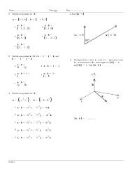
Lecture Notes 3: the three defs of the tangent space

Reading. Ch. 3 of Lee. Warner.
M is an abstract manifold. We have defined the tangent space to M via curves.
We are going to give two other definitions. All three are used in the subject and
one freely switches back and forth between the three.
Whatever the definition, the tangent space to M at a point p ∈ M must enjoy
the following properties. (1) it is a real vector space of dimension n = dim(M)
(2) it is intrinsically attached to M.
‘Intrinsic’ has two more-or-less equivalent meanings in differential geometry and
topology: (a) coordinate independent,
(b): equivariant under mappings: if F : M → N is a smooth map between
manifolds, then there should be defined, in a ‘natural’ way, a linear map dF (p) :
T p M → T F (p) N between tangent spaces.
The three definitions are:
Definition 1. Via curves.
Definition 2. Via derivations acting on functions
Definition 3. Via coordinates.
Definition 1 is the one we have given already.
We recall it. Define an equivalence relation among the smooth curves passing
through p. A tangent vector will be an equivalence class. This definition is the
most ‘geometric’ of the three, but sometimes the most difficult to compute with.
Definition. A smooth curve c through p is a map c : (−ɛ, ɛ) → M with c(0) = p.
Definition. Two smooth curves c, ˜c through p “agree to first order” if, in some
coordinate chart φ containing p their coordinate images agree to first order as curves
in R n :
φ ◦ c(t) = φ ◦ ˜c(t) + O(t 2 )
Definition. [Curve def of tangent space.] A tangent vector at p is an equivalence
class of curves passing through p. The tangent space is the set of all such equivalence
classes of curves.
The following lemma shows that this definition is ‘intrinsic’ in the sense (a).
Lemma. Suppose c, ˜c are two curves through p which agree to 1st order in some
chart φ. Then they agree to 1st order in any compatible chart.
Proof. Since c, ˜c agree to 1st order in the chart φ we have
φ ◦ c(t) = a + vt + O(t 2 )
φ ◦ ˜c(t) = a + vt + O(t 2 )
where a = φ(p). Let ψ be another chart, and g = ψ ◦ φ −1 Then ψ ◦ c = gφ ◦ c, ψ ◦
φc(t) = g ◦ φ ◦ ˜c(t) So that
φ ◦ c(t) = g(a + vt + O(t 2 )) = g(a) + [dg(a)v]t + O(t 2 )
φ ◦ ˜c(t) = g(a + vt + O(t 2 )) = g(a) + [dg(a)v]t + O(t 2 )
where we have used the fact that g is differentiable, and we have used the chain
rule to Taylor expand out g(a + vt + O(t 2 )). The two curves in the new coordinate
system still agree to 1st order. QED
Definition 2 of the tangent space. Via derivations.
1

2
Write C ∞ (M) for the space of all smooth functions on M. It is forms a commutative
algebra over the reals. We can add, and multiply functions, and scalar
multiply them.
Definiton. A derivation at p is an R linear map C ∞ (M) → R which is a derivation
in Leibnitz’s sense:
v[fg] = f(p)v[g] + g(p)v[f]
In other words: it is a linear functional for which the product rule works.
Definition. The tangent space to M at p is the space of derivations at p.
That this definiton is intrinsic is clear. We did not use coordinates to define it.
It is also obviously a vector space, since we can add derivations and multiply them
by real numbers. But the dimension of this vector space is not obvious. Is it finite?
Maybe there are too many functions? Or is it zero? How do we know a manifold
has ANY globally defined functions?
Exercise. If f and g agree in a nbhd of p and v is a derivation at p, then
v[f] = v[g].
Prop. If f is smooth defined in a coord nbhd of p, then it can be smoothly
extended to all of M.
Pf. Bump functions.
Cor. The value of v[f] is well-defined when f is defined on a nbhd of p, rather
than all of M.
( Rmk. Smooth Urysohn lemma. )
Cor. to exercise. Let U be any nbhod of p and consider the space C ∞ (U) of
smooth functions on To answer this last question will lead us to bump functions,
an important tool later on.
Definition 3 of the tangent space. via coordinates.
Consider all charts ψ α : U α ⊂ M → R n containing p, so that p ∈ U α . For each
such chart introduce a copy of R n , denoted by R n α, and form the disjoint union of
all these vector spaces. :
∐
{α:p∈U α}
. The funny symbol ∐ indicates DISJOINT union. Define an equivalence relation
∼ on this disjoint union by declaring v α ∈ R n α, and v β ∈ R n β
to be equivalent:
v α ∼ v β : iff d(ψ β ◦ ψα −1 )(ψ α (p))v α = v β . Then define T p M = ∐ {α:p∈U α} Rn α/ ∼.
This definition is clearly intrinsic according to notion (a) of ‘intrinsic’, since we
have divided out by all choice of charts. It is also clearly a vector space of dimension
n. Fix any one chart ψ α : U α ⊂ M− → R n . Then every [v] ∈ T p M has a unique
representative v α ∈ R n α so that R N ∼ α = T p M.
Pros and cons. This is the definition closest to the way computations are done.
It is the ugliest definition.
Bases in the various definitions. Standard notation. Equivalences between defintions.
Let x i be coordinates defined in a nbhd of p. Thus, some coordinate chart ψ :
U ⊂ M → R n is written out as ψ(q) = (x 1 (q), . . . , x n (q)). In all three definitions,
∂
these coordinates define a basis
∂x
, i = 1, . . . , n for T i p M. Thus a typical element
of T p M can be uniquely expressed as Σv i ∂
∂x
with v i ∈ R.
i
R n α

3
Basis in definition 1. Consider the coordinate x i -curve γ i . By this we mean
the curve in R n parallel to the x i axis and through the point corresponding to p:
thus:γ i (t) is defined by x j (t) = x j 0 , xi (t) = x i 0 + t, where x i 0 are the coordinates of
p. Then ∂
∂x
means the equivalence class of the curve ψ −1 (γ i i ).
Basis in definiton 2. If f ∈ C ∞ (M) then f ◦ ψ −1 : R n → R can be written (by a
slight abuse of notation) as f(x 1 , . . . , x n ). The derivation
∂
∂x
is the usual partial
i
∂
derivative:
∂x
[f] = ∂f
i ∂x i
∂
Basis in definition 3.
∂x
is the vector whose representative in the chart for
i
ψ = ψ α , is the vector e i = (0, . . . 0, 1, 0, . . .) ∈ R n α.
Equivalences of definitons.
Def 1 to 2. To define a derivation v from a curve c we set v[f] = ( d dt | t=0(f(c(t)).
Note: R−→M c
−→R
f
Coordinate computations shows c ↦→ v is well-defined on the level of equivalence
classes: if c 1 ∼ c 2 then ( d dt | t=0(f(c 1 (t)) = ( d dt | t=0(f(c 1 (t)). A coordinate computation
also shows that the map c ′ (0) → v is linear. If v = Σv i ∂
∂x
we compute, using
i
the chain rule that indeed:
v[f] = Σv i ∂
∂x i [f]
as it should.
Definition 2 corresponds to the directional derivative of vector calculus.
Def 1 to Def 3. We went from 1 to 3 when we showed that the equivalence class
of def 1 was chart-independent. (The lemma following the explanation of def 1:
write the curve in a coord chart. Its first order derivative is the tangent vector as
represented in that chart. ) Conversely, given a chart φ α : U α → R n = R n α with
P 0 corresponding to p, the inverse image under φ α of the curve P 0 + tv ∈ R n α is the
curve whose equivalence class represents v.
Def 3 to 2. The vector v = (v 1 , . . . v n ) ∈ R n α represents the derivation Σv i ∂
1.
More on Def 2. Why is the space of derivations based at p spanned by the
It is not even clear that this space of derivations is finite-dimensional.
∂x i .
∂
∂x i ?
Define bump functions. Discuss bump fns. Extending fns. Why we can think of
x i as fns on all of M.
Impossibility for cx mfds.
2. Derivations. Maximal ideals. Cotangent space.
We state some algebraic consequences of the definition. Let v be a derivation at
p, and let m p ⊂ C ∞ (M) be the subalgebra of functions vanishing at p.
Fact 1. v[c] = 0, c a constant function.
Proof: 1 = 1 · 1, so v[1] = 1v[1] + 1v[1] = 2v[1], implying that v[1] = 0. Now
v[c] = cv[1].
Consequence. v[f] = v[f − f(p)].
3.
Fact 2. If h = m 2 p then v[h] = 0.
Proof h ∈ m 2 p means h = fg for some f, g ∈ m p . Then v[h] = f(p)v[g]+g(p)v[f] =
0 + 0 since f(p) = g(p) = 0.

4
Proposition 0.1. v defines a linear map m p /m 2 p → R and is uniquely determined
by this map.
Proof: By fact 1 the value of v is determined by its values on m p . Any linear
map L : E → F between vector spaces descends canonically to a ‘quotient map”
E/ker(L) → F , and, if we know ker(L), then L is uniquely determined by this
quotient map.
3.
Fact 3. m p /m 2 p is a finite-dimensional vector space of dimension n.
Proof of Fact 3. The n coordinates are the 1st order Taylor expansion of a
function. In detail, use coordinates x i , i = 1, . . . , n centered at p. NOTE: “Centered
at p” means that x i (p) = 0.) Then Fact 2 transfers to the same statement regarding
m 0 ⊂ C ∞ (R n ). Expand f in terms of the x i : f = Σa i x i + O(|x| 2 ). We must show
that the remainder term O(|x| 2 ) is in m p . This is easily seen from
Lemma 0.2 (Hadamard’s lemma. ). Let f be a smooth function vanishing at
0 ∈ R n . Then we can write f = Σx i g i (x 1 , . . . , x n ) where the g i are smooth functions
satisfying g(0) = ∂f
∂x
| i 0
Proof of Hadamard. Write f(x) = f(0) + ∫ d
dt
out the integral to obtain f(x) = Σx i g i (x) where g i (x) = ∫ 1
f(tx)dt Use f(0) = 0 and expand
∂f
∂x
(tx)dt. QED (also
i
see, Lee, appendix).
End of proof of Fact 3. Hadamard’s lemma asserts that by subtracting off the
linear Taylor expansion, Σa i x i from f we obtain a function in m 2 0.
Definition. m p /m 2 p is called the “space of covectors” at p or the cotangent bundle
at p and is denoted by T ∗ p M.
Then the proposition asserts that the tangent space T p M (viewed as derivations)
is canonically dual to T ∗ p M.
Discussion.
There is a long tradition of recovering and better understanding a manifold,
variety, topological space,... by way of algebras of functiosn on it.
the correspondence p ↦→ m p ⊂ C ∞ (M) embeds M as a family of maximal ideals
within C ∞ (M).
Perhaps the most striking is in the subject of C ∗ -algebras , the theorem called
the Gelfand-Naimark theorem. Let M be a compact Hausdorff space and A the
space C 0 (M, C) of continous complex-valued functions on M, It is a commutative
algebra over C. The sup norm, and the operation f ↦→ ¯f , gives A the structure of
what is known as a C ∗ -algebra.
Gelfand-Naimark Theorem. Every commutative C ∗ algebra is C 0 (M, C) for some
compact Hausdorff space M.
The space M in the Gelfand-Naimark theorem is built out of “multiplicative
linear functionals” and forms the “spectrum” of A. Conversely, given M, the associated
“multiplicative linear functional” is evaluation at p: f ↦→ f(p), a map from
A → C. The kernel of this map corresponds to our m p .
Algebraic geometry. The subject begins by studying the zero locuses of polynomial
functions. These zero locuses are called “varieties”. Varieties are very often
manifolds, and are always manifolds at most of their points – like our cone or cross.
An essential theme in algebraic geometry is the traffic back and forth between the
variety and the algebra of polynomial functions defined on the variety. The variety
0

5
is reconstructed out of the algebra, as the space of maximal ideals in the algebra.
Our definition of the cotangent space and tangent space work in the algebraic setting,
even over arbitrary rings (!) and are called the Zariski (co)tangent space.