Diffusion Manual Outline
Diffusion Manual Outline
Diffusion Manual Outline

You also want an ePaper? Increase the reach of your titles
YUMPU automatically turns print PDFs into web optimized ePapers that Google loves.
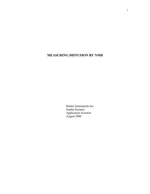
1<br />
MEASURING DIFFUSION BY NMR<br />
Bruker Instruments Inc.<br />
Sophie Kazanis<br />
Application Scientist<br />
August 2000
2<br />
Table of Contents<br />
Chapter 1<br />
Section 1.1<br />
Section 1.2<br />
Section 1.3<br />
Chapter 2<br />
Chapter 3<br />
Section 3.1<br />
Section 3.2<br />
Section 3.3<br />
Section 3.4<br />
Introduction to <strong>Diffusion</strong><br />
Introduction<br />
Some Theory<br />
Measuring <strong>Diffusion</strong><br />
Hardware and Probe Configuration<br />
Measuring <strong>Diffusion</strong><br />
Preparation<br />
Acquisition<br />
DOSY Data Analysis using ILT<br />
DOSY Data Analysis using XWINNMR:<br />
Fitting <strong>Diffusion</strong> Coefficients<br />
Appendix
3<br />
Chapter 1<br />
Section 1.1<br />
Introduction to <strong>Diffusion</strong><br />
Introduction<br />
Self-diffusion is a measure of the translational motion of a molecule. <strong>Diffusion</strong> is<br />
closely related to molecular size as illustrated by the Stokes-Einstein equation seen<br />
below:<br />
D = k T<br />
f<br />
where k is the Boltzman constant, T is the temperature and f is the friction coefficient.<br />
For the simple case of a spherical particle of a hydrodynamic radius r s in a solvent of<br />
viscosity η, the friction factor is given by f = 6 π η r s<br />
Translational diffusion can be used to determine the size and shape of individual<br />
molecules as well as molecular aggregates. This provides an excellent way of analyzing<br />
complex mixtures without having to physically separate out each individual component.<br />
Pulsed-field gradient (PFG) NMR can be used to measure translational diffusion<br />
by applying externally controlled magnetic field gradients. These gradients spatially<br />
encode the position of each nuclear spin. This spatial distribution can be decoded after<br />
waiting a short time by applying a second gradient. If the waiting time is very short<br />
between the encoding and decoding gradients the spins will not have had a chance to<br />
change position and in turn the magnetization will refocus without a net phase change.<br />
However the spins that have moved during the waiting time between the encoding and<br />
decoding steps will acquire a net phase change. The summation of the accumulated<br />
phases over the entire sample will lead to partial cancellation of the observable<br />
magnetization and hence an attenuation of the NMR signal. This signal attenuation is<br />
dependent on the strength of the applied gradients, the time between the gradients<br />
(diffusion time) and the diffusion coefficient of the molecules under study.<br />
Section 1.2<br />
Some Theory<br />
Nuclear spins within a homogeneous magnetic field precess at the Larmor<br />
frequency according to the equation<br />
ω o = γB o<br />
where ω o is the Larmor frequency<br />
γ is the gyromagnetic ratio and<br />
B o is the strength of the magnetic field
4<br />
An external field gradient, g, can be described by the equation<br />
g = ∂ B z i + ∂ B z j + ∂ B z k<br />
∂x ∂y ∂z<br />
where i, j and k are unit vectors in the x, y and z direction.<br />
When an external gradient is applied the magnetic field at a specific set of coordinate can<br />
be described as the sum of the main field and the field due to the applied gradient:<br />
B = B o + g . r<br />
where r describes the position of a specific nuclear spin<br />
The direction of the magnetic field is usually defined as the z-direction. Here we will<br />
limit our discussion to the case of a gradient applied in the z-direction. The description<br />
of the external gradient can be simplified to be<br />
g z = g . k<br />
Applying a gradient along the z direction induces change in the phase angle for each spin<br />
at a specific z coordinate. This change in phase can be described as follows:<br />
φ (z) = γ g z z t<br />
where γ is the gyromagnetic ratio, g z is the gradient strength at position z, z indicates the<br />
position of the spin at time t.<br />
The total change in phase angle of a particular spin at time, t, after a gradient has been<br />
applied is a combination of the phase change induced by the static field as well as the<br />
contribution from the applied gradient.<br />
φ (z) = γ B o t + γ g z z t<br />
Now if you apply two gradients of equal and opposite strength and duration successively<br />
after an initial 90 degree pulse, the first gradient will dephase the magnetization and the<br />
second gradient will refocus the magnetization.<br />
90º<br />
¾!UVVM<br />
ÅV²³
5<br />
Figure 1.1 Simple gradient echo experiment<br />
φ 1(z) is the phase changed by the first gradient and φ 2(z) is the phase change induced by<br />
the second gradient. The total phase accumulation is the sum of φ 1(z) and φ 2(z) .<br />
φ 1 (z) + φ 2 (z) = φ Tot(z)<br />
If the spins have not changed position during the dephasing and rephasing gradients the<br />
net total phase change will be zero and full signal should be observed.<br />
φ Tot(z) = 0<br />
In order to refocus the chemical shift evolution that occurs while the magnetization is on<br />
the transverse plane we can place a 180 degree pulse between the two gradients. Here<br />
again if the spins have not changed position during the encoding and decoding steps the<br />
net total phase change will be zero, φ Tot(z) = 0 (Note that since the 180 degree pulse<br />
inverts the magnetization, the second gradient now has to be equal in amplitude, duration<br />
and sign as the first gradient).<br />
90º 180º<br />
¾!$VVM<br />
ÅV²²<br />
Figure 1.2 Simple gradient spin echo experiment
6<br />
Section 1.3<br />
Measuring <strong>Diffusion</strong><br />
The simplest experiment that can be used to measure diffusion is the Stejskal and Tanner<br />
pulsed field gradient spin echo pulse sequence shown below.<br />
90ºx 180ºy<br />
¾!VVV$VUVWO<br />
<br />
= <br />
ÅV²VUV²UUV<br />
Figure 1.3 The Stejskal and Tanner PFG spin echo pulse sequence. On 1 H the thin<br />
black solid line denotes a 90º pulse and the thick solid black line denotes a 180º . G z<br />
gradients for coding and decoding are denoted by a sine bell.<br />
In this experiment a gradient is applied right after the first 90 degree pulse has been<br />
executed. The spins experience a change in the phase angle proportionate to the<br />
amplitude of the applied gradient. After a time ∆/2 a 180 degree pulse is applied which<br />
refocuses chemical shifts. The molecules are allowed to diffuse for a period of ∆. The<br />
second gradient then allows the magnetization to be refocused and the FID is<br />
subsequently recorded. Since the spins are allowed to move during the diffusion time, ∆,<br />
the net total phase change after the second gradient summed over the entire sample will<br />
not be zero. This leads to an attenuation in the observed signal.<br />
In order to measure the diffusion coefficients a series of experiments with varying echo<br />
time, ∆,=are recorded. The intensity of the signals should decrease with increasing echo<br />
time. There are two disadvantages with this method. First, the overall length of each<br />
experiment is different. Your are also usually limited with the range of echo times that<br />
can be used to obtain significant signal intensity. Secondly, the contribution of T 2<br />
relaxation during the echo time while the magnetization is on the transverse plane varies<br />
from experiment to experiment.<br />
The same effect can be obtained and the disadvantages avoided by varying the gradient<br />
amplitude while keeping the duration of the gradient constant. The overall length of each<br />
experiment will remain constant. The signal intensity will decrease with increasing<br />
gradient strength. Since the echo time for a series of experiments is the same the affects<br />
of T 2 relaxation should remain constant within a given series of experiments.
7<br />
Figure 1.4 Shows the attenuation of signal with increasing gradient strength<br />
The decrease in signal intensity as a function of gradient strength can be described by the<br />
general equation<br />
I (q) = I o e-Dq2∆’<br />
where D is the diffusion coefficient<br />
∆’ = ∆ – δ/3 where<br />
∆ is the diffusion time and δ is a correction factor for finite gradients<br />
q = γgδ<br />
γ is the gyromagnetic ratio<br />
g is the amplitude of the applied gradient<br />
δ is the duration of the applied gradient<br />
A plot of I (q) versus q2 ∆’ yields an exponential decay curve which is fitted to obtain the<br />
diffusion coefficient.
8<br />
Figure 1.5 A plot of the change of signal intensity with increasing gradient strength<br />
<strong>Diffusion</strong> experiments are conveniently performed in a two dimensional fashion. A<br />
pseudo two dimensional experiment is constructed with chemical shift on the horizontal<br />
axis and (distribution of ) diffusion coefficients on the vertical axis. This is known as<br />
diffusion ordered NMR spectroscopy or DOSY.<br />
The DOSY experiment analyzes and concisely displays the data that is acquired with a<br />
series of PFG NMR experiments outlined above. The signal attenuation at each chemical<br />
shift is inverted by approximate inverse Laplace transforms (ILT) to generate a<br />
distribution of diffusion coefficients at a particular chemical shift.<br />
Figure 1.6 An example of a DOSY experiment with diffusion coefficients on the on the<br />
vertical axis and chemical shifts on the horizontal axis.
10<br />
Chapter 2<br />
Hardware and Probe Configuration<br />
To execute PFG NMR experiments your console must be equipped with a gradient<br />
control unit, GCU, and a gradient amplifier. The GREAT 1/10, GAB and single axis<br />
ACCUSTAR (10 A) amplifiers can only generate z gradients where as the ACCUSTAR<br />
and GREAT 3/10 (10 A) amplifiers can generate x, y and z gradients.<br />
All DOSY experiments can be performed with z axis gradients.<br />
The high resolution NMR probe must have a gradient coil which is actively shielded to<br />
minimize eddy currents. The gradient coil must be able to provide a constant gradient<br />
over the entire length of the active sample volume. Standard high resolution probes can<br />
generate up to 65 G/cm with a 10 A amplifier along the z axis and up to 50 G/cm along<br />
the x and y axis.<br />
Higher powered (40 A) amplifiers are available but are not recommended for standard<br />
high resolution applications.<br />
For very demanding diffusion applications special diffusion probes are available. These<br />
probes can produce up to 30 G/ cm /A or up to 1.2 kG with a 40 A amplifier. These<br />
probes have reduced high resolution performance specifications.
11<br />
Chapter 3:<br />
Section 3.1:<br />
Measuring <strong>Diffusion</strong><br />
Preparation<br />
1. You must use a 1D sequence to optimize the DOSY acquisition parameters. It is<br />
recommended that you begin with the ledbp2s1d sequence. This sequence uses<br />
bipolar gradients which help eliminate any background gradients that would lead<br />
to additional unwanted echoes. Make sure that minimum number of scans which<br />
fulfill the phase cycle are used. The initial range of diffusion time, d20, should be<br />
in the range of 50-100ms. Begin with a 1ms gradient pulse, p16, and with a<br />
gradient strength of 2%. This 1d spectrum is used as a reference.<br />
2. Increase the gradient strength to 95% and monitor the attenuation of the NMR<br />
signal. The remaining signal intensity should be approximately 2-5% of the<br />
original (reference) signal intensity. If this is not the case adjust the acquisition<br />
parameters accordingly until the above criteria are observed.<br />
3. The first variable to try adjusting is p16. For bipolar gradients p16 can be <<br />
2.5ms and for monopolar gradients p16 < 5ms. The second variable that can be<br />
modified is d20, the diffusion time.<br />
4. Once the parameters have been adjusted accordingly, you may proceed with the<br />
2D DOSY acquisition.<br />
5. If ILT will be used for the data analysis then the maximum gradient strength for<br />
the particular probe must be calibrated (see Avance GRASP users manual) and<br />
put into the file “XWINNMRHOME/conf/instr/gradient_calib”. You can do this<br />
manually from a unix shell (Notepad file Windows NT) or you can use<br />
XWINNMR by going into setpre and editing the Grad.calib.const value. The<br />
maximum gradient strength is about 60 G/cm for probes with only z-axis<br />
gradients. Probes with x,y,z-axis gradients the have maximum z-gradients of<br />
about 65 G/cm and x,y-gradients of 50 G/cm.<br />
Section 3.2:<br />
Acquisition<br />
1. Create a new dataset (edc). In the acquisition window (eda) change the PARMOD to<br />
2D.<br />
2. In the ased submenu edit the appropriate values for the pulse widths, delays,<br />
constants and sweep width.<br />
3. Execute the au program dosy by typing xau dosy. You will be asked the following<br />
questions:
12<br />
Enter the first gradient amplitude: 5<br />
Enter the final gradient amplitude: 90<br />
Enter the number of points: 16<br />
Do you want to begin the acquisition:<br />
y<br />
Typing xau dosy 5 90 16 y in the command line will have the same effect as answering<br />
the questions above.<br />
The dosy au program creates a binary linear gradient ramp file which is stored in the<br />
“~/exp/stan/nmr/lists/gp” directory and is called dramp. For this particular example the<br />
file dramp will contain a 16 step ramp starting from 5% gradient amplitude and ending<br />
with 95% and it will also automatically begin the acquisition.<br />
Dosy also creates a “vdlist” which is stored with the experiment data. This vdlist<br />
contains the gradient amplitudes in G/cm for each step of the gradient ramp. The entries<br />
in the vdlist are adjusted for the amplitude of the gradients at each step and they are also<br />
scaled to account for the fact that sine shaped gradients are used instead of rectangular<br />
gradients for the acquisition of the experiment.<br />
Other AU Programs: dosyq and dosylist<br />
The au program dosyq is similar to the au program dosy except that it creates a binary<br />
“squared” ramp file called dramp. In this case the gradient amplitudes follow a square<br />
root function. This way you would observe a linear response of signal amplitude as a<br />
function of gradient amplitude.<br />
The au program dosylist recalculates the ramp file but only stores the “vdlist” where the<br />
gradient amplitudes in G/cm units are stored. It uses the status parameters found in the<br />
experiment. You should use this au program if you did not use dosy or dosyq to start<br />
your experiment and you wish to the use ILT to process the data.
13<br />
Section 3.3:<br />
DOSY Data Analysis using ILT<br />
Figure 3.1 A comparison of the Fourier transform where the FID in the time domain is converted to an<br />
NMR experiment in the frequency domain versus the inverse Laplace transform which converts the<br />
attenuation of signal at a specific chemical shift to a distribution of diffusion coefficients.<br />
After the DOSY data has been acquired you must process it by typing xf2 on the<br />
command line. It might be necessary to apply a phase correction to the data. You should<br />
observe that the intensity of the signal amplitude decreases with increasing gradient<br />
strength.<br />
You can obtain the inverse Laplace transform (ILT) of the attenuation in signal intensity<br />
by using the Bruker ILT program.<br />
1. Type ilt on the command line. The following screen will appear.
14<br />
2. Fill out the table accordingly.<br />
First you must choose the type of pulse sequence that was used.<br />
STE is the stimulated echo pulse program (stegs1s, ledgs2s)<br />
STEbp is a stimulated echo with bipolar gradients (ledbpgs2s)<br />
DSTE is the double stimulated echo (dstegs3s)<br />
DSTEbp is a double stimulated echo with bipolar gradients<br />
Enter the new process number (procno) where the DOSY analysis will be stored. Make<br />
sure you do not overwrite the raw data.<br />
The Row start to end should indicate how many steps were in the gradient ramp file.<br />
The Col start to end should indicate the number of points representing each spectrum<br />
that will undergo the inverse Laplace transform.<br />
The threshold value indicates the lower intensity limit at a particular chemical shift for<br />
which the transformation will occur.<br />
There are three different modes offered for data analysis. The option monoexp will fit<br />
the decay of intensity at each chemical shift with single exponential decay curve and<br />
yield a single diffusion coefficient per chemical shift. This option should be used if it is<br />
known that the components within a mixture are monodisperse and a single diffusion<br />
coefficient exists. The option biexp will fit the decay of intensities with biexponential<br />
decay curve and yield a possible two diffusion coefficients per chemical shift. This<br />
option should be used if it is thought that the diffusion at each chemical shift cannot be<br />
adequately represented by a single diffusion coefficient. This would be the case if it is<br />
known that there is chemical shift overlap with various components within a mixture.<br />
The option CONTIN is used when the components within a mixture are known to be<br />
polydisperse and are known to diffuse with a distribution of coefficients. Examples of<br />
polydisperse species include polymers, micelles and droplets. So within a DOSY<br />
spectrum such species will yield Gaussian distribution of diffusion coefficients with<br />
increased width.<br />
Fit offset should be set to yes if signal intensity has not decayed to 2-5% of the original<br />
signal intensity.<br />
SI (F1) indicates how much zero filling takes place in the diffusion dimension of the<br />
pseudo 2D DOSY experiment.<br />
The value in Sdev indicates a factor by which the standard deviation is multiplied. If the<br />
experimental data has a relatively high signal to noise ratio the Sdev value can be reduced<br />
(0.01) to obtain sharper Gaussian distributions of diffusion coefficients
15<br />
Solutions bounds indicates the range of fitting parameters which are proportional to the<br />
diffusion constants. It is recommended to use the ranges 1 to 1000 or 0.1 to 100.<br />
Solution grid selects the scale in the indirect (2 nd ) (F1) dimension.<br />
3. Once the table has been filled out click on OK and read the appropriate process<br />
number.<br />
Note: Inverse Laplace transforms are very time consuming. In particular the CONTIN<br />
calculation can take several minutes to complete. If the dataset is displayed before the<br />
end of the calculation then partially transformed data will be displayed.
16<br />
Section 3.4:<br />
DOSY Data Analysis Using XWINNMR:<br />
Fitting <strong>Diffusion</strong> Coefficients<br />
1. After you have processed (xf2) and phase corrected the data you will observe a<br />
DOSY spectrum similar to the one shown below.<br />
2. Under the submenu Analysis choose Relaxation [ T1/T2 ].<br />
3. Type rspc in the command line or under Process choose Read SMX slice for<br />
peak selection. You will now observe the first 1D spectrum from the 2D dataset.<br />
4. In the utilities submenu define the peaks for which you wish to fit a diffusion<br />
curve. Select defpoints and using the middle mouse button define the peaks. Save the<br />
peak file and return to the Relaxation [ T1/T2 ] menu from the Analysis submenu.
17<br />
5. Set up the parameters for the fitting. Under the Process menu choose Setup T1<br />
parameters or type edt1 on the command line. The following screen will appear.<br />
6. Set “FITTYPE” to intensity if you only wish to use the attenuation in signal<br />
intensity for the fitting .<br />
Set “FCTYPE” to vargrad. This indicates that the diffusion experiment was<br />
acquired using variable gradients but constant time deltas.<br />
Most of the other parameters should be fine. Make sure that<br />
GAMMA (4.258 e+03 Hz/G for proton), LITDEL (p16 gradient duration) and<br />
BIGDEL (d20 diffusion time) are set correctly for that particular experiment.<br />
7. Edit the “EDGUESS”. The following screen will appear.<br />
The very top line of this menu shows the formula that is used for the fitting routine.
18<br />
The equation is in the form<br />
I (q) = I o e-Dq2∆’<br />
The fitting routine will therefore fit a single exponential decay. The fit should be quite<br />
accurate if there is a single species is represented for a particular peak at a specific<br />
chemical shift.<br />
The values GC1IO and GC1D represent the estimates for the amplitudes and the<br />
diffusion coefficients. Since the amplitudes are normalized to one GC1IO is set to 1.<br />
The estimate for the diffusion coefficient should be set to the correct order of magnitude<br />
in units m2/s. GC1D is set to 1e-09 m2/s. The values SC1IO and SC1D represent the<br />
initial steps for the fitting routing and they are usually set to on tenth of the corresponding<br />
values in the left column. SC1IO = 0.1 and SC1D = 1e-10 m2/s. Save the guesses and<br />
return to the edt1 menu. Now save the edt1 menu.<br />
8. Under the Process menu you can now Pick intensities exactly at point or you<br />
can type pdo on the command line. A graph of your data points as a function of variable<br />
gradient strength will be displayed.<br />
9. To fit the data, choose Multi-component fit from the Process menu or type<br />
simfit on the command line.
19<br />
10. To view the results on the screen the “CURPRINT” in the edo menu must be set<br />
to “$screen”. If “CURPRINT” is set to a specific printer you will get a printout of the<br />
results. The results are also stored in the processed data directory in a file called<br />
simfit.out.<br />
11. To eliminate a corrupted data point you put the cursor into the graphical window.<br />
Move the cursor to the point which you wish to remove and press the middle mouse<br />
button. Double click on the left button to exit the elimination function. Now you can fit<br />
the data again by typing simfit at the command line.
20<br />
Appendix<br />
Pulse Sequences and Corresponding Gradient Programs<br />
stegs1s<br />
The pulsed field gradient stimulated echo (PFG-STE) diffusion pulse sequence is most<br />
commonly used to measure diffusion and it is shown below. The advantage of this<br />
sequence over the classic PFG spin echo sequence is that the second 90º pulse stores the<br />
magnetization in the z direction. Now the major relaxation mechanism during the<br />
relatively long diffusion time is T 1 instead of T 2 as in the case of spin echo sequence.<br />
This is advantageous since T 1 is usually greater than T 2 for most molecules. This<br />
minimizes transverse relaxation and J-modulation affects. The subsequent 90º pulse<br />
brings the magnetization back into the xy plane for observation.<br />
90ºx 90º-x 90ºx<br />
¾!V!Vl!WUN<br />
ÅV²V)UV²UUV<br />
Figure 4.1.1 The PFG-STE pulse sequence. On 1 H the black solid lines denote 90º<br />
pulses. On Gz sine shaped gradients for coding and decoding are unfilled and spoil<br />
gradients for artifact suppression are filled with diagonal lines.<br />
The Bruker pulse program for this experiment is shown below.<br />
;stegs1s<br />
;avance-version<br />
;2D sequence for diffusion measurement using stimulated echo<br />
;using 1 spoil gradient<br />
#include <br />
#include <br />
"d31=d20-p1*2-p16-d16-p19-d16"<br />
"ds=l20"<br />
1 ze<br />
2 d1 BLKGRAD<br />
3 50u UNBLKGRAD<br />
p1 ph1<br />
GRADIENT(cnst21)<br />
d16<br />
p1 ph2<br />
GRADIENT2(cnst22)<br />
d16<br />
d31<br />
p1 ph3<br />
GRADIENT(cnst21)<br />
d16
21<br />
4u BLKGRAD<br />
go=2 ph31<br />
d1 wr #0 if #0 zd<br />
lo to 3 times td1<br />
exit<br />
ph1= 0 0 0 0 2 2 2 2 1 1 1 1 3 3 3 3<br />
ph2= 1 3 0 2<br />
ph3= 1 3 0 2<br />
ph31=0 0 2 2 2 2 0 0 3 3 1 1 1 1 3 3<br />
;pl1 : f1 channel - power level for pulse (default)<br />
;p1 : f1 channel - high power pulse<br />
;p16: gradient pulse (little DELTA)<br />
;p19: gradient pulse 2 (spoil gradient)<br />
;d1 : relaxation delay; 1-5 * T1<br />
;d16: delay for gradient recovery<br />
;d20: diffusion time (big DELTA)<br />
;d31: d20 - p1*2 - p16 - d16 - p19 - d16<br />
;l20: dummy scans (ds)<br />
;NS: 8 * n<br />
;DS: l20<br />
;td1: number of experiments<br />
;MC2: use xf2 and ilt for processing<br />
;use gradient program (GRDPROG) : Ste1s<br />
;use gradient ratio: cnst22<br />
; -13.17<br />
;use AU-program dosy or dosyq to calculate gradient-file dramp<br />
The acquisition parameters are described at the end of the pulse sequence.<br />
P1 and pl1 are the 1 H 90º pulse width and power level<br />
P16 is the duration of the encoding/decoding gradient<br />
P19 is the duration of the spoiler gradient (1-3ms)<br />
D16 is the gradient recovery time (500us)<br />
D20 is the length of the diffusion time<br />
Cnst21 represents the gradient strength of the encoding/decoding gradient. The value of<br />
cnst21 varies according to the starting and ending strength and the number of<br />
experiments indicated in the dosy au program that helps you to set up the experiment.<br />
Cnst22 is the gradient strength of the spoiler gradient and is usually set to an odd number<br />
to diminish the chances of refocusing unwanted magnetization.<br />
The gradient program that is associated with this experiment, Ste1s, is shown below:<br />
Ste1s<br />
loop l20<br />
{<br />
p16 { (0) | (0) | (0),sin(2,100) }<br />
{ (0) | (0) | (0) }<br />
p19 { (0) | (0) | (0),sin(cnst22,100) }<br />
{ (0) | (0) | (0) }<br />
p16 { (0) | (0) | (0),sin(2,100) }<br />
{ (0) | (0) | (0) }<br />
}<br />
loop td1 <br />
{<br />
loop ns<br />
{<br />
p16 { (0) | (0) | (0),sin(100,100)*dramp(100) }
22<br />
}<br />
}<br />
{ (0) | (0) | (0) }<br />
p19 { (0) | (0) | (0),sin(cnst22,100) }<br />
{ (0) | (0) | (0) }<br />
p16 { (0) | (0) | (0),sin(100,100)*dramp(100) }<br />
{ (0) | (0) | (0) }<br />
The first part of this gradient program is used during the acquisition of the dummy scans.<br />
The number of dummy scans is indicated by the variable L20.<br />
p16 { (0) | (0) | (0),sin(2,100) }<br />
indicates a sine shaped gradient pulse of 2% strength made up of 100 points.<br />
During the course of the experiment the gradient strength is varied by the value of the<br />
dramp. Dramp is set when you execute the au program ‘dosy’ and specify the starting<br />
and ending gradient strength along with the number of experiments.<br />
p16 { (0) | (0) | (0),sin(100,100)*dramp(100) }
23<br />
ledgs2s<br />
Eddy currents can effect the stimulated echo diffusion experiment. Eddy current effects<br />
occur more readily at higher gradient strengths. Using shaped gradient pulses can reduce<br />
the effects of eddy currents by decreasing the rate of change of the magnetic field when a<br />
gradient pulse is switched on or off. But using shaped gradients does not always<br />
completely alleviate the problem. The stimulated echo experiment is most affected by<br />
the eddy currents produced by the final gradient pulse. The LED, longitudinal eddy<br />
current delay sequence was developed to help minimize these affects. The fourth 90º<br />
pulse stores magnetization in the longitudinal direction, thus allowing the eddy currents<br />
to decay during the period Te (T). The fifth 90º pulse brings the magnetization back in to<br />
the transverse plane so that the FID can be acquired. The PFG-LED pulse sequence is<br />
shown below:<br />
90ºx 90º-x 90ºx 90º-x 90ºx<br />
¾!!Vl!!z!M<br />
ÅV²)UV²)UUUV<br />
Figure 4.1.2 The PFG-LED pulse sequence. On 1 H the black solid lines denote 90º pulses. On Gz sine<br />
shaped gradients for coding and decoding are unfilled and spoil gradients for artifact suppression are filled<br />
with diagonal lines.<br />
The Bruker pulse program for this experiment is shown below.<br />
;ledgs2s<br />
;avance-version<br />
;2D sequence for diffusion measurement using stimulated<br />
; echo and LED<br />
;using 2 spoil gradients<br />
;A.S. Altieri, D.P. Hinton & R.A. Byrd,<br />
; J. Am. Chem Soc. 117, 7566-7567 (1995)<br />
#include <br />
#include <br />
"d30=d21-p19-d16-4u"<br />
"d31=d20-2*p1-p16-d16-p19-d16"<br />
"ds=l20"<br />
1 ze<br />
2 d1 BLKGRAD<br />
3 50u UNBLKGRAD<br />
p1 ph1<br />
GRADIENT(cnst21)<br />
d16<br />
p1 ph1<br />
GRADIENT2(cnst22)<br />
d16<br />
d31<br />
p1 ph1<br />
GRADIENT(cnst21)<br />
d16<br />
p1 ph2
24<br />
GRADIENT2(cnst23)<br />
d16<br />
d30<br />
4u BLKGRAD<br />
p1 ph3<br />
go=2 ph31<br />
d1 wr #0 if #0 zd<br />
lo to 3 times td1<br />
exit<br />
ph1= 0 0 0 0 0 0 0 0 2 2 2 2 2 2 2 2<br />
1 1 1 1 1 1 1 1 3 3 3 3 3 3 3 3<br />
ph2= 0 0 0 0 2 2 2 2 2 2 2 2 0 0 0 0<br />
1 1 1 1 3 3 3 3 3 3 3 3 1 1 1 1<br />
ph3= 0 1 2 3 2 3 0 1 2 3 0 1 0 1 2 3<br />
1 2 3 0 3 0 1 2 3 0 1 2 1 2 3 0<br />
ph31=0 1 2 3 0 1 2 3 2 3 0 1 2 3 0 1<br />
1 2 3 0 1 2 3 0 3 0 1 2 3 0 1 2<br />
;pl1 : f1 channel - power level for pulse (default)<br />
;p1 : f1 channel - high power pulse<br />
;p16: gradient pulse (little DELTA)<br />
;p19: gradient pulse 2 (spoil gradient)<br />
;d1 : relaxation delay; 1-5 * T1<br />
;d16: delay for gradient recovery<br />
;d20: diffusion time (big DELTA)<br />
;d21: eddy current delay (Te)<br />
[5 ms]<br />
;d30: d21 - p19 - d16 - 4u<br />
;d31: d20 - p1*2 - p16 - d16 - p19 - d16<br />
;l20: dummy scans (ds)<br />
;NS: 8 * n<br />
;DS: l20<br />
;td1: number of experiments<br />
;MC2: use xf2 and ilt for processing<br />
;use gradient program (GRDPROG) : Led2s<br />
;use gradient ratio: cnst22 : cnst23<br />
; -13.17 : -17.13<br />
;use AU-program dosy or dosyq to calculate gradient-file dramp<br />
The acquisition parameters are described at the end of the pulse sequence.<br />
P1 and pl1 are the 1 H 90º pulse width and power level<br />
P16 is the duration of the encoding/decoding gradient<br />
P19 is the duration of the spoiler gradient (1-3ms)<br />
D16 is the gradient recovery time (500us)<br />
D20 is the length of the diffusion time<br />
D21 is the length of the eddy current delay<br />
Cnst21 represents the gradient strength of the encoding/decoding gradient. The value of<br />
cnst21 varies according to the starting and ending strength and the number of<br />
experiments indicated in the dosy au program that helps you to set up the experiment.<br />
Cnst22 and cnst23 are the gradient strength of the spoiler gradients and are usually set to<br />
an odd number to diminish the chances of refocusing unwanted magnetization.<br />
The gradient program associated with this experiment is Ledgs and is shown below:<br />
Ledgs<br />
loop l20<br />
{<br />
p16 { (0) | (0) | (0),sin(2,100) }
25<br />
{ (0) | (0) | (0) }<br />
p19 { (0) | (0) | (0),sin(cnst22,100) }<br />
{ (0) | (0) | (0) }<br />
p16 { (0) | (0) | (0),sin(2,100) }<br />
{ (0) | (0) | (0) }<br />
p19 { (0) | (0) | (0),sin(cnst23,100) }<br />
{ (0) | (0) | (0) }<br />
}<br />
loop td1 <br />
{<br />
loop ns<br />
{<br />
p16 { (0) | (0) | (0),sin(100,100)*dramp(100) }<br />
{ (0) | (0) | (0) }<br />
p19 { (0) | (0) | (0),sin(cnst22,100) }<br />
{ (0) | (0) | (0) }<br />
p16 { (0) | (0) | (0),sin(100,100)*dramp(100) }<br />
{ (0) | (0) | (0) }<br />
p19 { (0) | (0) | (0),sin(cnst23,100) }<br />
{ (0) | (0) | (0) }<br />
}<br />
}
26<br />
ledbp2s<br />
Another good way to decrease eddy current affects that are induced by a short gradient is<br />
to replace the gradient pulse with two gradient pulses of opposite polarity and half the<br />
duration separated by a 180º 1H pulse. This (Gz--180º--(-Gz) composite pulse<br />
combination self compensates for the induced eddy currents. The LED experiment with<br />
the bipolar pulse pairs should help reduce most of the eddy current effects. The BPP-<br />
LED sequence is shown below:<br />
90º 180º 90º 90º 180º 90º 90º<br />
¾!'!Vl!'!z!M<br />
ÅV²³)VU²³)UVUU<br />
Figure 4.1.3 The BPP-LED pulse sequence. On 1 H the thin solid black lines denote 90º<br />
pulses and the thicker solid black lines denote 180º. On Gz sine shaped gradients for<br />
coding and decoding are unfilled and spoil gradients for artifact suppression are filled<br />
with diagonal lines.<br />
The Bruker pulse program for this sequence is shown below:<br />
;ledbpgs2s<br />
;avance-version<br />
;2D sequence for diffusion measurement using stimulated<br />
; echo and LED<br />
;using bipolar gradient pulses for diffusion<br />
;using 2 spoil gradients<br />
;D. Wu, A. Chen & C.S. Johnson Jr.,<br />
; J. Magn. Reson. A 115, 260-264 (1995).<br />
#include <br />
#include <br />
"p2=p1*2"<br />
"d30=d21-p19-d16-4u"<br />
"d31=d20-p1*2-p2-p16*2-d16*2-p19-d16"<br />
1 ze<br />
2 d1 BLKGRAD<br />
3 50u UNBLKGRAD<br />
p1 ph1<br />
GRADIENT(cnst21)<br />
d16<br />
p2 ph1<br />
GRADIENT(-cnst21)<br />
d16<br />
p1 ph2<br />
GRADIENT2(cnst22)<br />
d16<br />
d31<br />
p1 ph3<br />
GRADIENT(cnst21)<br />
d16<br />
p2 ph1<br />
GRADIENT(-cnst21)
27<br />
d16<br />
p1 ph4<br />
GRADIENT2(cnst23)<br />
d16<br />
d30<br />
4u BLKGRAD<br />
p1 ph5<br />
go=2 ph31<br />
d1 wr #0 if #0 zd<br />
lo to 3 times td1<br />
exit<br />
ph1= 0<br />
ph2= 0 0 2 2<br />
ph3= 0 0 0 0 2 2 2 2 1 1 1 1 3 3 3 3<br />
ph4= 0 2 0 2 2 0 2 0 1 3 1 3 3 1 3 1<br />
ph5= 0 0 0 0 2 2 2 2 1 1 1 1 3 3 3 3<br />
ph31=0 2 2 0 2 0 0 2 3 1 1 3 1 3 3 1<br />
;pl1 : f1 channel - power level for pulse (default)<br />
;p1 : f1 channel - 90 degree high power pulse<br />
;p2 : f1 channel - 180 degree high power pulse<br />
;p16: gradient pulse (little DELTA)<br />
;p19: gradient pulse 2 (spoil gradient)<br />
;d1 : relaxation delay; 1-5 * T1<br />
;d16: delay for gradient recovery<br />
;d20: diffusion time (big DELTA)<br />
;d21: eddy current delay (Te)<br />
[5 ms]<br />
;d30: d21 - p19 - d16 - 4u<br />
;d31: d20 - p1*2 - p2 - p16*2 - d16*2 - p19 - d16<br />
;l20: dummy scans (ds)<br />
;NS: 8 * n<br />
;DS: l20<br />
;td1: number of experiments<br />
;MC2: use xf2 and ilt for processing<br />
;use gradient program (GRDPROG) : Ledbp2s<br />
;use gradient ratio: cnst22 : cnst23<br />
; -13.17 : -17.13<br />
;use AU-program dosy or dosyq to calculate gradient-file dramp<br />
The acquisition parameters are described at the end of the pulse sequence.<br />
P1 and pl1 are the 1 H 90º pulse width and power level<br />
P16 is the duration of the encoding/decoding gradient which should be set to ½ the value<br />
of used in the ledgs2s pulse program<br />
P19 is the duration of the spoiler gradient (1-3ms)<br />
D16 is the gradient recovery time (500us)<br />
D20 is the length of the diffusion time<br />
D21 is the length of the eddy current delay<br />
Cnst21 represents the gradient strength of the encoding/decoding gradient. The value of<br />
cnst21 varies according to the starting and ending strength and the number of<br />
experiments indicated in the dosy au program that helps you to set up the experiment.<br />
Cnst22 and cnst23 are the gradient strength of the spoiler gradients and are usually set to<br />
an odd number to diminish the chances of refocusing unwanted magnetization.<br />
The gradient program associated with this experiment is Ledbp2s and is shown below:<br />
Ledbp2s
28<br />
loop l20<br />
{<br />
p16 { (0) | (0) | (0),sin(2,100) }<br />
{ (0) | (0) | (0) }<br />
p16 { (0) | (0) | (0),-sin(2,100) }<br />
{ (0) | (0) | (0) }<br />
p19 { (0) | (0) | (0),sin(cnst22,100) }<br />
{ (0) | (0) | (0) }<br />
p16 { (0) | (0) | (0),sin(2,100) }<br />
{ (0) | (0) | (0) }<br />
p16 { (0) | (0) | (0),-sin(2,100) }<br />
{ (0) | (0) | (0) }<br />
p19 { (0) | (0) | (0),sin(cnst23,100) }<br />
{ (0) | (0) | (0) }<br />
}<br />
loop td1 <br />
{<br />
loop ns<br />
{<br />
p16 { (0) | (0) | (0),sin(100,100)*dramp(100) }<br />
{ (0) | (0) | (0) }<br />
p16 { (0) | (0) | (0),-sin(100,100)*dramp(100) }<br />
{ (0) | (0) | (0) }<br />
p19 { (0) | (0) | (0),sin(cnst22,100) }<br />
{ (0) | (0) | (0) }<br />
p16 { (0) | (0) | (0),sin(100,100)*dramp(100) }<br />
{ (0) | (0) | (0) }<br />
p16 { (0) | (0) | (0),-sin(100,100)*dramp(100) }<br />
{ (0) | (0) | (0) }<br />
p19 { (0) | (0) | (0),sin(cnst23,100) }<br />
{ (0) | (0) | (0) }<br />
}<br />
}<br />
;ledbpgs2s1d<br />
;avance-version<br />
;1D sequence for diffusion measurement using stimulated<br />
; echo and LED<br />
;using bipolar gradient pulses for diffusion<br />
;using 2 spoil gradients<br />
;D. Wu, A. Chen & C.S. Johnson Jr.,<br />
; J. Magn. Reson. A 115, 260-264 (1995).<br />
#include <br />
#include <br />
"p2=p1*2"<br />
"d30=d21-p19-d16-4u"<br />
"d31=d20-p1*2-p2-p16*2-d16*2-p19-d16"<br />
1 ze<br />
2 d1 BLKGRAD<br />
3 50u UNBLKGRAD<br />
p1 ph1<br />
GRADIENT(cnst21)<br />
d16<br />
p2 ph1<br />
GRADIENT(-cnst21)<br />
d16<br />
p1 ph2<br />
GRADIENT2(cnst22)<br />
d16<br />
d31<br />
p1 ph3<br />
GRADIENT(cnst21)<br />
d16<br />
p2 ph1<br />
GRADIENT(-cnst21)<br />
d16<br />
p1 ph4<br />
GRADIENT2(cnst23)
29<br />
d16<br />
d30<br />
4u BLKGRAD<br />
p1 ph5<br />
go=2 ph31<br />
d1 wr #0<br />
exit<br />
ph1= 0<br />
ph2= 0 0 2 2<br />
ph3= 0 0 0 0 2 2 2 2 1 1 1 1 3 3 3 3<br />
ph4= 0 2 0 2 2 0 2 0 1 3 1 3 3 1 3 1<br />
ph5= 0 0 0 0 2 2 2 2 1 1 1 1 3 3 3 3<br />
ph31=0 2 2 0 2 0 0 2 3 1 1 3 1 3 3 1<br />
;pl1 : f1 channel - power level for pulse (default)<br />
;p1 : f1 channel - 90 degree high power pulse<br />
;p2 : f1 channel - 180 degree high power pulse<br />
;p16: gradient pulse (little DELTA)<br />
;p19: gradient pulse 2 (spoil gradient)<br />
;d1 : relaxation delay; 1-5 * T1<br />
;d16: delay for gradient recovery<br />
;d20: diffusion time (big DELTA)<br />
;d21: eddy current delay (Te)<br />
[5 ms]<br />
;d30: d21 - p19 - d16 - 4u<br />
;d31: d20 - p1*2 - p2 - p16*2 - d16*2 - p19 - d16<br />
;l20: dummy scans (ds)<br />
;NS: 8 * n<br />
;DS: l20<br />
;td1: number of experiments<br />
;MC2: use xf2 and ilt for processing<br />
;use gradient program (GRDPROG) : Ledbp2s1d<br />
;use gradient ratio: cnst22 : cnst23<br />
; -13.17 : -17.13<br />
The acquisition parameters are described at the end of the pulse sequence.<br />
P1 and pl1 are the 1 H 90º pulse width and power level<br />
P16 is the duration of the encoding/decoding gradient which should be set to ½ the value<br />
of used in the ledgs2s pulse program<br />
P19 is the duration of the spoiler gradient (1-3ms)<br />
D16 is the gradient recovery time (500us)<br />
D20 is the length of the diffusion time<br />
D21 is the length of the eddy current delay<br />
Cnst21 represents the gradient strength of the encoding/decoding gradient.<br />
Cnst22 and cnst23 are the gradient strength of the spoiler gradients and are usually set to<br />
an odd number to diminish the chances of refocusing unwanted magnetization.<br />
The gradient program associated with this experiment is Ledbp2s1d and is shown below:<br />
loop ns<br />
{<br />
p16 { (0) | (0) | (0),sin(cnst21,100) }<br />
{ (0) | (0) | (0) }<br />
p16 { (0) | (0) | (0),-sin(cnst21,100) }<br />
{ (0) | (0) | (0) }
30<br />
}<br />
p19 { (0) | (0) | (0),sin(cnst22,100) }<br />
{ (0) | (0) | (0) }<br />
p16 { (0) | (0) | (0),sin(cnst21, 100) }<br />
{ (0) | (0) | (0) }<br />
p16 { (0) | (0) | (0),-sin(cnst21,100) }<br />
{ (0) | (0) | (0) }<br />
p19 { (0) | (0) | (0),sin(cnst23,100) }<br />
{ (0) | (0) | (0) }
31<br />
dstegs3s<br />
Temperature gradients that exist or are induced within a sample during the course of an<br />
experiment can create convection currents. These convection currents interfere with<br />
accurate measurement of the diffusion coefficients. This occurs because the diffusion<br />
velocities of the molecules vary with temperature. Most temperature gradients can be<br />
minimized by using a temperature control unit. However, if you are working well below<br />
ambient temperature and are using solvents that have very low viscosity it is quite<br />
difficult to avoid convection currents. Under these circumstances it is recommended that<br />
you use a pulse sequence which is insensitive to maintaining a constant diffusion velocity<br />
for the molecules such as the double stimulated echo sequence (DSTE) shown below:<br />
¾!!Vq!U!Vq!!Vz!M<br />
ÅV²)VU²²)UV²)UUUU<br />
Figure 3.1.1 The PFG-DSTE with LED pulse sequence. On 1 H the black solid lines<br />
denote 90º pulses. On Gz sine shaped gradients for coding and decoding are unfilled and<br />
spoil gradients for artifact suppression are filled with diagonal lines.<br />
The Bruker pulse program for this sequence is shown below:<br />
;dstegs3s<br />
;avance-version<br />
;2D sequence for diffusion measurement using double stimulated<br />
; echo and LED<br />
;using 3 spoil gradients<br />
;A. Jerschow & N. Mueller, J. Magn. Reson. A 123, 222-225 (1996)<br />
;A. Jerschow & N. Mueller, J. Magn. Reson. A 125, 372-375 (1997)<br />
#include <br />
#include <br />
"d30=d21-p19-d16-4u"<br />
"d31=d20-p1*2-p16-d16-p19-d16"<br />
"ds=l20"<br />
1 ze<br />
2 d1 BLKGRAD<br />
3 50u UNBLKGRAD<br />
p1 ph1<br />
GRADIENT(cnst21)<br />
d16<br />
p1 ph2<br />
GRADIENT2(cnst22)<br />
d16<br />
d31<br />
p1 ph3<br />
GRADIENT(cnst21)<br />
d16<br />
GRADIENT(cnst21)<br />
d16<br />
p1 ph4<br />
GRADIENT2(cnst23)<br />
d16<br />
d31<br />
p1 ph5
32<br />
GRADIENT(cnst21)<br />
d16<br />
p1 ph6<br />
GRADIENT2(cnst24)<br />
d16<br />
d30<br />
4u BLKGRAD<br />
p1 ph7<br />
go=2 ph31<br />
d1 wr #0 if #0 zd<br />
lo to 3 times td1<br />
exit<br />
ph1= 0 1 2 3<br />
ph2= 0<br />
ph3= 2 3<br />
ph4= 2 2 2 2 0 0 0 0<br />
ph5= 0<br />
ph6= 0<br />
ph7= 0<br />
ph31=0 0 2 2 2 2 0 0<br />
;pl1 : f1 channel - power level for pulse (default)<br />
;p1 : f1 channel - high power pulse<br />
;p16: gradient pulse (little DELTA)<br />
;p19: gradient pulse 2 (spoil gradient)<br />
;d1 : relaxation delay; 1-5 * T1<br />
;d16: delay for gradient recovery<br />
;d20: diffusion time (big DELTA)<br />
;d21: eddy current delay (Te)<br />
[5 ms]<br />
;d30: d21 - p19 - d16 - 4u<br />
;d31: d20 - p1*2 - p16 - d16 - p19 - d16<br />
;l20: dummy scans (ds)<br />
;NS: 8 * n<br />
;DS: l20<br />
;td1: number of experiments<br />
;MC2: use xf2 and ilt for processing<br />
;use gradient program (GRDPROG) : Dste3s<br />
;use gradient ratio: cnst22 : cnst23 : cnst24<br />
; -13.17 : -17.13 : -15.37<br />
;use AU-program dosy or dosyq to calculate gradient-file dramp<br />
;the gradients serve the following purpose:<br />
; GRADIENT(cnst21) first STE dephase<br />
; GRADIENT2(cnst22) spoiler<br />
; GRADIENT(cnst21) first STE rephase<br />
; GRADIENT(cnst21) second STE dephase<br />
; GRADIENT2(cnst23) spoiler<br />
; GRADIENT(cnst21) second STE rephase<br />
; GRADIENT2(cnst24) LED with spoiler<br />
The acquisition parameters are described at the end of the pulse sequence.<br />
P1 and pl1 are the 1 H 90º pulse width and power level<br />
P16 is the duration of the encoding/decoding gradient<br />
P19 is the duration of the spoiler gradient (1-3ms)<br />
D16 is the gradient recovery time (500us)<br />
D20 is the length of the diffusion time<br />
D21 is the length of the eddy current delay<br />
Cnst21 represents the gradient strength of the encoding/decoding gradient. The value of<br />
cnst21 varies according to the starting and ending strength and the number of<br />
experiments indicated in the dosy au program that helps you to set up the experiment.
33<br />
Cnst22, cnst23 and cnst24 are the gradient strength of the spoiler gradients and are<br />
usually set to an odd number to diminish the chances of refocusing unwanted<br />
magnetization.<br />
The gradient program associated with this experiment is Dste3s and is shown below:<br />
loop l20<br />
{<br />
p16 { (0) | (0) | (0),sin(2,100) }<br />
{ (0) | (0) | (0) }<br />
p19 { (0) | (0) | (0),sin(cnst22,100) }<br />
{ (0) | (0) | (0) }<br />
p16 { (0) | (0) | (0),sin(2,100) }<br />
{ (0) | (0) | (0) }<br />
p16 { (0) | (0) | (0),sin(2,100) }<br />
{ (0) | (0) | (0) }<br />
p19 { (0) | (0) | (0),sin(cnst23,100) }<br />
{ (0) | (0) | (0) }<br />
p16 { (0) | (0) | (0),sin(2,100) }<br />
{ (0) | (0) | (0) }<br />
p19 { (0) | (0) | (0),sin(cnst24,100) }<br />
{ (0) | (0) | (0) }<br />
}<br />
loop td1 <br />
{<br />
loop ns<br />
{<br />
p16 { (0) | (0) | (0),sin(100,100)*dramp(100) }<br />
{ (0) | (0) | (0) }<br />
p19 { (0) | (0) | (0),sin(cnst22,100) }<br />
{ (0) | (0) | (0) }<br />
p16 { (0) | (0) | (0),sin(100,100)*dramp(100) }<br />
{ (0) | (0) | (0) }<br />
p16 { (0) | (0) | (0),sin(100,100)*dramp(100) }<br />
{ (0) | (0) | (0) }<br />
p19 { (0) | (0) | (0),sin(cnst23,100) }<br />
{ (0) | (0) | (0) }<br />
p16 { (0) | (0) | (0),sin(100,100)*dramp(100) }<br />
{ (0) | (0) | (0) }<br />
p19 { (0) | (0) | (0),sin(cnst24,100) }<br />
{ (0) | (0) | (0) }<br />
}<br />
}