Focus on deep and shallow convection, and turbulence - cmmap

<strong>Focus</strong> on deep and shallow convection,
and turbulence
Steve Krueger and Chin-Hoh Moeng
Princeville, Kauai, Hawaii
20 February 2007

10,000 km
Scales of Atmospheric Motion
1000 km 100 km 10 km 1 km 100 m 10 m
Planetary
waves
Extratropical
Cyclones
Cumulonimbus
Mesoscale
clouds
Convective Systems
Cumulus
clouds
Turbulence =>
Global Climate Model
(GCM)
Cloud System Resolving
Model (CSRM)
Large Eddy Simulation
(LES) Model
Multiscale Modeling Framework

from Arakawa and Jung (2003)

Boundary layer clouds in
deep-convection-resolving models (DCRMs)
• DCRMs are CRMs with horizontal
grid sizes of 4 km or more.
• Used in MMF, GCRMs (global
CRMs), and tropical cyclone
models.
• In MMF and GCRMs, DCRMs are
expected to represent all types of
cloud systems.
• However, many cloud-scale
circulations are not resolved by
DCRMs.
• Representations of SGS
circulations currently used in
DCRMs can be improved.

Boundary layers in
deep precipitating convective cloud systems
• Tropical convective cloud
systems may organize too
readily in the FRCGC GCRM
and in MMF GCMs.
• Possible causes:
• Convectively-generated cold
pools are too strong.
• Boundary layer stabilization
due to shallow convection is
under-estimated.
• Poor horizontal resolution may
contribute to both.

Shallow cumulus clouds
and mesoscale organization
• Typical DCRMs grid sizes are
too large to resolve shallow
cumulus.
• A DCRM with a suitable SGS
parameterization should be
able to represent shallow
cumulus and resolved
mesoscale organization.
• LES can be used to provide a
benchmark simulation.

Outline of this talk
•Introduction
•Objectives of focus
•Scope and
relationship to old
WGs
•Science issues
•Meeting the objectives

Introduction
• Objectives of focus:
Improve the representation of SGS convection and turbulence in deepconvection-resolving
models (DCRMs), for use in MMFs, GCRMs, and NWP.
• Scope and relationship to old WGs:
• Extensions, evaluations, and applications of the prototype MMF(s)
• Development and testing of improved parameterizations of microphysics and
radiation for use in CSRMS, MMFs, and GCRMs
• Development and testing of improved parameterizations of boundary layer
clouds and turbulence for use in CSRMS, MMFs, and GCRMs
• Accelerated improvement of conventional parameterizations
• Optimal use of computational and data storage resources
• Knowledge-transfer to climate modeling centers
• Knowledge transfer to numerical weather prediction centers

Science Issues
Representation of the following cloud systems and boundary layer
regimes in DCRMs:
• Deep precipitating convective
• Transition from shallow to deep convection
• Diurnal cycle of shallow convection over land
• Trade cumulus
• Marine stratocumulus
• Cold-air outbreaks over mid-latitude oceans
• Convective plumes from leads during winter
• Boundary layers over inhomogenous surfaces or terrain

Meeting the Objectives
Develop and test improved representations of SGS convection and turbulence
in DCRMs.
• Proposed parameterizations
• PDF/HOC: Cheng & Xu, Lappen & Randall
• Two-scale MMF: DCRM plus boundary-layer-eddy-resolving model (ERM)
• Additional physics to be included
• Effects of surface inhomogeniety (elevation, land surface properties): both
resolved by the DCRM and SGS
• Proposed evaluation methods
• Analysis of and comparison to benchmark simulations
• Comparison to observational datasets

Boundary-layer Clouds in a Multiscale
Modeling Framework (MMF)
Anning Cheng , Kuan-Man Xu , Yali Luo,
Jiundar Chern, and Wei-Kuo Tao

Joint PDF of total water and liquid
water potential temperature
LES PDF
double Gaussian PDF
single Gaussian PDF

Continental shallow cumuli (ARM)
LES PDF
double Gaussian PDF
single Gaussian PDF

Randall, D. A., Q. Shao, and C.-H. Moeng 1992: A
Second-Order Bulk Boundary-Layer Model. J. Atmos.
Sci., 49, 1903-1923.
Lappen, C.-L, and D. A. Randall, 2001: Towards a unified
parameterization of the boundary layer and moist
convection. Part I. A new type of mass-flux model. J.
Atmos. Sci., 58, 2021-2036.
These papers show that:
• Mass flux methods can be married with higher-order
closure.
• With this approach, the triple-moment terms of the
second moment equations can either advect or
diffuse, depending on the regime.

Proposed Evaluation Methods
•Benchmark simulations
•Large-domain LES (e.g., 100 km x 100 km domain,
0.1 km grid size)
•Compare to DCRM results using various SGS
parameterizations.
•Compare to SCM results.
•Analyze results to gain insight into scale interactions,
etc.

High-Resolution Simulation of Shallow-to-Deep
Convection Transition over Land
(Khairoutdinov and Randall 2006)
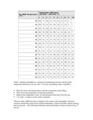
Figure 8. PDF of cloud size as a function of height shown for three different simulation times. Mean and
standard deviations are shown by the white and yellow lines, respectively.
150 km x 150 km, 100 m grid size, 6 h

Grid-size dependence in a large domain LES
•RICO trade wind cumulus case: 19 Jan 2005
•Control simulation: 100 m horizontal grid size, 40 km x
40 km domain, 24 h simulation
•Grid-size dependence simulations: 500 m, 1000 m,
2000 m, 4000 m horizontal grid sizes, otherwise
unchanged from control
•Next: stereo images of clouds at 12 h

100 m

500 m

1000 m

2000 m

4000 m

100 m

500 m

1000 m

2000 m

4000 m

100 m
Figure 12:

Avg’d to 500 m
log 10
of Liquid Water Path (g/m 2 ), hour 12
40
35
3
30
2.5
25
2
y (km)
20
1.5
15
10
1
5
0.5
0
0 5 10 15 20 25 30 35 40
x (km)

Avg’d to 1000 m
log 10
of Liquid Water Path (g/m 2 ), hour 12
40
35
3
30
2.5
25
2
y (km)
20
1.5
15
10
1
5
0.5
0
0 5 10 15 20 25 30 35 40
x (km)

1000 m
log 10
of Liquid Water Path (g/m 2 ), hour 12
40
35
3
30
2.5
25
2
y (km)
20
1.5
15
10
1
5
0.5
0
0 5 10 15 20 25 30 35 40
x (km)

1
Cloud Fraction
0.9
0.8
0.7
cloud fraction
0.6
0.5
0.4
0.3
100 m
500 m
0.2 1000 m
2000 m
4000 m
0.1
0 200 400 600 800 1000 1200 1400
time (min)
Figure 1:

last 6 hrs 100 m 500 m 1000 m 2000 m 4000 m
cloud fraction 0.18 0.28 0.58 0.87 0.94
LWP (g/m 2 ) 23.9 26.7 46.0 69.1 96.7
precip rates (mm/hr) 0.003 0.022 0.050 0.038 0.070
Table 1: Statistics from the last 6 hrs

5000
4500
4000
Water Vapor Mixing Ratio
100 m
500 m
1000 m
2000 m
4000 m
3500
height (m)
3000
2500
2000
1500
1000
500
0
0 2 4 6 8 10 12 14 16
water vapor mixing ratio (g/kg)
Figure 3:

5000
4500
4000
Cloud Water Mixing Ratio
100 m
500 m
1000 m
2000 m
4000 m
3500
height (m)
3000
2500
2000
1500
1000
500
0
0 0.02 0.04 0.06 0.08 0.1 0.12 0.14 0.16 0.18 0.2
cloud water mixing ratio (g/kg)
Figure 2:

5000
4500
4000
Rain Water Mixing Ratio
100 m
500 m
1000 m
2000 m
4000 m
3500
height (m)
3000
2500
2000
1500
1000
500
0
0 1 2 3 4 5 6 7
rain water mixing ratio (g/kg)
x 10 !3
Figure 4:

Proposed Evaluation Methods
•Observational datasets
•High-resolution cloud properties from satellites:
MODIS, ISCCP, etc
•Vertical structure of clouds: CloudSat, ARM MMCR,
TRMM
•High-resolution hourly precipitation from rain gage
and unbiased radar
•Surface mesonet observations of T, RH, p, u, v
•Aircraft-based measurements during field
experiments