View - Martin Kröger - ETH Zürich

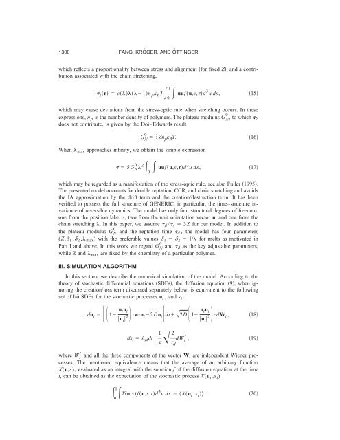
1300 FANG, KRÖGER, AND ÖTTINGER
which reflects a proportionality between stress and alignment for fixed Z, and a contribution
associated with the chain stretching,
2 r c1n p k B T
0
1
uuf u,s,rd 3 uds,
15
which may cause deviations from the stress-optic rule when stretching occurs. In these
expressions, n p is the number density of polymers. The plateau modulus G N
0 , to which 2
does not contribute, is given by the Doi–Edwards result
G N
0
3
5 Zn p k B T. 16
When max approaches infinity, we obtain the simple expression
5G N
0
2
0
1
uuf u,s,rd 3 uds,
17
which may be regarded as a manifestation of the stress-optic rule, see also Fuller 1995.
The presented model accounts for double reptation, CCR, and chain stretching and avoids
the IA approximation by the drift term and the creation/destruction term. It has been
verified to possess the full structure of GENERIC, in particular, the time–structure invariance
of reversible dynamics. The model has only four structural degrees of freedom,
one from the position label s, two from the unit orientation vector u, and one from the
chain stretching . In this paper, we assume d / s 3Z for our model. In addition to
0
the plateau modulus G N and the reptation time d , the model has four parameters
(Z, 1 , 2 , max ) with the preferable values 1 2 1/ for melts as motivated in
0
Part I and above. In this work we regard G N and d as the key adjustable parameters,
while Z and max are fixed by the chemistry of a particular polymer.
III. SIMULATION ALGORITHM
In this section, we describe the numerical simulation of the model. According to the
theory of stochastic differential equations SDEs, the diffusion equation 9, when ignoring
the creation/loss term discussed separately below, is equivalent to the following
set of Itô SDEs for the stochastic processes u t , and s t :
du t 1 u t u t
u t 2 •–u t 2Du tdt2D 1 u t u t
u t 2 •dW t ,
ds t ṡ tot dt 1 2 d
dW t ,
18
19
where W t and all the three components of the vector W t are independent Wiener processes.
The mentioned equivalence means that the average of an arbitrary function
X(u,s), evaluated as an integral with the solution f of the diffusion equation at the time
t, can be obtained as the expectation of the stochastic process X(u t ,s t )
1
0 Xu,sfu,s,td 3 uds Xu t ,s t .
20