Single Particle Analysis Tutorial - Xmipp

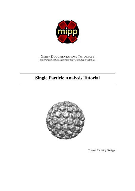
XMIPP DOCUMENTATION: TUTORIALS 

(http://xmipp.cnb.csic.es/twiki/bin/view/Xmipp/Tutorials) 

Single Particle Analysis Tutorial 

Thanks for using Xmipp

Xmipp Documentation 

SPA Tutorial 

Contents 

1 General introduction 4 

1.1 Download and Install . . . . . . . . . . . . . . . . . . . . . . . . . . . . . . . 4 

1.2 Welcome to Xmipp! . . . . . . . . . . . . . . . . . . . . . . . . . . . . . . . . 4 

1.3 Formats . . . . . . . . . . . . . . . . . . . . . . . . . . . . . . . . . . . . . . 5 

1.3.1 Metadata Files . . . . . . . . . . . . . . . . . . . . . . . . . . . . . . 5 

1.3.2 EMX Files . . . . . . . . . . . . . . . . . . . . . . . . . . . . . . . . 6 

1.3.3 2D images, 3D volumes, 2D stacks and 3D stacks . . . . . . . . . . . . 6 

1.4 Standardized protocols . . . . . . . . . . . . . . . . . . . . . . . . . . . . . . 7 

2 Your first 3D reconstruction in Xmipp 8 

2.1 Download data and getting started . . . . . . . . . . . . . . . . . . . . . . . . 8 

2.2 Preprocessing . . . . . . . . . . . . . . . . . . . . . . . . . . . . . . . . . . . 10 

2.3 Particle Picking . . . . . . . . . . . . . . . . . . . . . . . . . . . . . . . . . . 16 

2.4 Particles . . . . . . . . . . . . . . . . . . . . . . . . . . . . . . . . . . . . . . 19 

2.5 Align+Classify . . . . . . . . . . . . . . . . . . . . . . . . . . . . . . . . . . 22 

2.6 Initial model . . . . . . . . . . . . . . . . . . . . . . . . . . . . . . . . . . . . 23 

2.7 Projection Matching . . . . . . . . . . . . . . . . . . . . . . . . . . . . . . . . 24 

3 Concluding remarks 29 

2



Intended audience 

This demo provides a general introduction to Xmipp 3.0 (X-window based Microscopy Image 

Processing Package). It is designed to introduce 3D image processing in electron microscopy 

to people without any prior knowledge of Xmipp, only limited knowledge about 3D-EM image 

processing, and with basic computer skills. 

We’d like to hear from you 

We have tested and verified the different steps described in this demo to the best of our knowledge, 

but since our programs are in continuous development you may find inaccuracies and 

errors in this text. Please, let us know about any error you find, as well as your suggestion for 

future editions by writing to xmipp@cnb.csic.es. 

3



1 General introduction 

1.1 Download and Install 

The first step before start working on your projects is to download and install Xmipp. You can 

download Xmipp from download. Details about installation can be found in how_to_install. 

1.2 Welcome to Xmipp! 

Xmipp was introduced to the scientific society more than a decade ago (Marabini et al., 1996). 

Originally it was written in C, but in 2004 it was completely re-implemented in a hierarchical 

structure of C++ libraries (Sorzano et al., 2004). In its current state (De la Rosa-Trevín et al., 

2013), Xmipp contains more than 200 stand-alone programs. 

Let’s have a first look at the Xmipp package. Open a Unix-like shell, and type: 

xmipp_ [+TAB] 

to see a list of all available Xmipp commands. You will see there are more than two hundreds 

different programs. Any Xmipp program may be called from the command line, and if you do 

not give any options, a limited description of its parameters is shown. Just try typing the name 

of any of them, for example: 

xmipp_reconstruct_wbp 

gives the following output to the screen: 

PROGRAM 

xmipp_reconstruct_wbp 

USAGE 

Generate 3D reconstruction from projections using the Weighted 

BackProjection algorithm. 

SEE ALSO 

angular_projection_matching, angular_discrete_assign, 

angular_continuous_assign 

OPTIONS 

-i 

selection file with input images and Euler angles 

[-o ] 

filename for output volume 

[-doc ] 

Ignore headers and get angles from this docfile 

[-radius ] 

Reconstruction radius. int=-1 means radius=dim/2 

The volume will be zero outside this radius 

[-sym ] 

Enforce symmetry 

[-weight] 

Use weights stored in image headers or the input 

metadata 

4



Common options 

[-gui] 

Show a GUI to launch the program. 

[-more] 

Show additional options. 

EXAMPLES 

xmipp_reconstruct_wbp -i images.sel -o reconstruction.vol 

This is the program to perform a 3D reconstruction using an algorithm called weighted backprojection. 

In case you want to obtain information about a Xmipp command but you do not know 

the exact program name you can use 

xmipp_apropos 

that searches for Xmipp programs that are related to some keywords, for example, 

xmipp_apropos -i reconstruct 

A complete list of the available programs may be found on the ListOfPrograms at the Xmipp 

(Wiki) website. The links on that page points to more detailed manual pages for each of the 

programs. This list can also be obtained in the console without 

xmipp_apropos -l 

Some programs are numerical-only and will run in the shell (i.e. xmipp_reconstruct_wbp 

program mentioned above). Other programs have a graphical interface (like xmipp_browser, 

the program to visualize images, volumes, self-organizing maps etc.), i.e. they will launch an 

additional window. There are several programs that have an implementation for parallel execution 

(using message-passing interface, MPI). The names of parallel programs always start with 

xmipp_mpi_. 

1.3 Formats 

1.3.1 Metadata Files 

In Xmipp metadata information (that can be thought as “data about data”) is transferred between 

programs using metadata files. Metadata files are handled by the metadata class. Metadata 

files uses the STAR (Self-defining Text Archiving and Retrieval) format. In a nutshell, the 

STAR format is a plain text format (i.e., human-readable) that defines tag-value pairs with few 

rules on the composition of the file: Xmipp metadata standard introduces several constrains to 

ease implementation. You can see an example of a metadata file and additional information in 

MetadataFiles. 

Metadata files are used to keep lists of images, lists of micrographs, correspondences between 

images and micrographs (from which micrograph each image has been taken from), lists of 

micrograph coordinates, 2D and 3D alignment parameters, CTF parameters, ... You can think of 

a Metadata file as a table in which you can add as many columns as you like. Each column has 

its own meaning. The list of columns available can be seen by typing xmipp_apropos -l 

-t labels. 

5



1.3.2 EMX Files 

Xmipp is commited to support EMX exchange format. Information related with this format can 

be seen here EMX 

1.3.3 2D images, 3D volumes, 2D stacks and 3D stacks 

Xmipp supports the following image file formats/extensions: 

For further information, please take a look to ImageFormats. 

Note that Xmipp also has specific functionality for format conversions (just type xmipp_image_convert). 

An important difference between Xmipp and other packages is that Xmipp avoids interpolating 

the images by storing geometrical information (for instance, 2D shifts, 3D Euler angles, ...) 

in metadata files. The original images are never touched during 2D or 3D alignment. Instead, 

metadata alignment or classification files are written containing all the geometrical information 

needed for constructing 2D or 3D models. Note that in Xmipp 2.4 this geometrical information 

was normally stored in the Spider image header. However, in Xmipp 3.0, the image header is 

not read and all geometrical information must be kept in metadatas. You can extract the image 

header to produce a metadata or viceversa using the program xmipp_image_header. Alternatively, 

you may use xmipp_transform_geometry (with the option --apply_transform) 

to produce interpolated images that can be used by other packages. xmipp_showj has an option 

to visualize metadatas and images with or without the geometrical information (Display→Apply 

geometry). 

For 3D volumes and 2D Stacks, Xmipp supports several file formats (see table above). Stacks 

of volumes are supported through Spider stacks. Additionally, any “header+raw data” format 

is supported through the # syntax (#xDim,yDim,[zDim],offset,datatype,[r]). In 

this syntax, after writing the filename, you describe the size of the image or volume, the offset in 

bytes to reach the raw data and the datatype. You can additionally indicate whether the endianess 

is reversed or not with respect to the machine default. For instance, let us assume we have an 

image with a format not supported by Xmipp. It has a header of 1040 bytes, the image size 

is 2048x2048 of unsigned 16 bits integers, and the endianness is reversed with respect to the 

machine, we may read this file by using for instance 

xmipp_showj -i myfile.myext#2048,2048,1,1040,uint16,r 

6



1.4 Standardized protocols 

The multitude of standalone Xmipp programs allows a broad functionality. Just by typing command 

line instructions, the user may devise its own data processing strategy. However, for novice 

users it may be hard to find out which program to use at each stage, while the more experienced 

users may repeat certain sequences of command-line instructions many times. Therefore, a 

higher-level layer has been added to Xmipp in the form of executable python scripts for the 

more popular image processing strategies in Xmipp (Scheres et al., 2008). To further ease their 

use, a graphical user-interface (GUI) has been developed (xmipp, xmipp_protocols or 

xp). Also see the GettingStarted Wiki page for more detailed information. 

Clicking the buttons for the distinct processing tasks will copy the standardized python scripts 

to your project directory inside a folder called Runs/, and open a GUI-window that allows to 

edit the parameters in the script headers and subsequent script execution. Besides scripts for job 

execution, also scripts that help in visualizing their results have been developed. 

In this demo, we will mainly work with the standardized python scripts. If you are planning 

on using Xmipp on a regular basis, it is probably a good idea to keep track of which individual 

Xmipp commands were executed by inspecting the log-files that are output by the different 

scripts (by default in a directory called Logs/). 

7



2 Your first 3D reconstruction in Xmipp 

Single Particle Analysis: Depending on the nature of each sample, different strategies 

must be chosen in order to obtain a 3D reconstruction. If the sample contains a single object, 

electron tomography should be chosen. Electron tomography allows 3D reconstruction of a 

single object after acquisition of tilt series. Conversely, when the sample is composed of multiple 

copies of the same object, such as proteins and macromolecular complexes, the strategy 

of data collection and 3D reconstruction is different and aims at the computation of a 3D average 

map. When the particles lack any particular symmetry, an approach named single particle 

analysis can be applied. This method consists in obtaining for each electron microscopy image, 

multiples projections of identical objects at different orientations. Therefore, to make a threedimensional 

reconstruction we combine these projections from a large number of particles in 

different orientations (Sorzano et al., 2007). In Fig. 1 we show a diagram that illustrates the 

single particle technique. 

Figure 1: Illustration of the basic principle of single particle analysis 

In this demo, we have used the single particle analysis approach to obtain a 3D reconstruction 

of a Bovine Papillomavirus. The EM images have been collected at 300 kV and a calibrated 

magnification of 56,588, giving a pixel size on the specimen of 1.237 Å (Wolf et al., 2010). 

Data have been kindly provided by ( Dr. Grigorieff’s Lab.) 

2.1 Download data and getting started 

Before proceed with this tutorial be sure that you have Xmipp (version 3.0 or newer) properly 

installed. Details about installation can be found in how_to_install. 

The data you will work on may be downloaded and extracted using the following commands: 

wget -nc \ 

http://xmipp.cnb.csic.es/Downloads/XmippDoc/3.0/xmipp3_intro.tgz 

tar -xvzf xmipp3_intro.tgz 

8



You may also see the “solution”, i.e., the same project with all protocols runs and a final 

reconstruction at 

wget -nc \ 

http://xmipp.cnb.csic.es/Downloads/XmippDoc/3.0/xmipp3_intro_solved.tgz 

After download and extract the data, you should have a folder named BPV_Project. This 

will be the project folder and working directory for executing all steps of this tutorial. Enter in 

the project folder by typing: 

cd BPV_Project 

Inside this folder you will find the file BPV_scale_filtered_windowed.vol and another 

folder InputData containing three sample micrographs in .mrc format. You can take a 

look of one micrograph as follows (See Fig 2): 

xmipp_showj InputData/BPV_1386.mrc 

To create the project and launch the main GUI you should type: 

xmipp_protocols 

After this you will be asked to confirm project creation: 

You are in directory: /gpfs/fs1/home/bioinfo/jvargas/BPV Do you want 

to CREATE a NEW PROJECT in this folder? [Y/n] Y 

Figure 2: Visualization of an input micrograph. 

9



Just type y, and the GUI main window will be launched (see Fig.3). The left panel contains 

different protocols grouped in categories. Clicking on a group will display a menu with protocols 

that can be selected to launch the corresponding GUI. You can see more about protocols GUI 

here . 

Figure 3: Xmipp protocols main GUI. 

2.2 Preprocessing 

• Import Micrographs 

The first step for obtaining the 3D reconstruction is to import our micrographs to our Xmipp 

project. To import the images press first on Micrographs button and then on Import 

Micrographs. After doing this, we will see the Import Micrographs GUI Fig. 4 

Modify the parameters of the Import Micrographs according to the ones shown in Fig. 

4. In the ’Micrographs directory’ you must indicate the folder where your micrograph files are 

stored. In ’Files to process’ the micrographs to process (if we use *.mrc, we are saying that we 

want to process all micrographs of type .mrc inside the folder InputData). Note that the icon 

permits detecting the files to process automatically. You can use a job queuing system if desired. 

This is useful on many large computer clusters, but if you are working on your own computer 

you will probably not have a queueing system. When you have completed the form, click on 

the Save & Execute button. After executing the protocol, it will appear in the main Xmipp 

GUI the following new information Fig. 5. 

If we press in the Analyze results button it will appear a new pop-up GUI that shows 

us the different imported micrographs Fig. 6 

10



Figure 4: Xmipp Import Micrographs GUI 

Figure 5: Xmipp GUI after processing Import Micrograph protocol 

11



Figure 6: Imported micrographs in the Xmipp project 

Figure 7: Visualization of Xmipp logs and stderr and stdout outputs. 

We also can view the logs, outputs and errors of the different Xmipp programs launched by 

the protocol pressing on the Output Files button Fig. 7 

12



• Screen Micrographs 

After importing the micrographs to your Xmipp project, you can perform the next processing 

step that consists in Screen Micrographs (Micrographs-> Screen Micrographs). 

This protocol is responsible of the CTF estimation process. In order to estimate the CTF, we 

will need some parameters describing the frequency region to be analyzed. The parameters 

shown in Fig. 8 are the adequate ones for this experiment. 

Figure 8: Xmipp Screen Micrographs GUI 

When the protocol finishes, you will have the CTF estimation results and you can observe the 

aberrations that occur in the microscope during image formation. This may be useful in order to 

discard bad micrographs. 

To observe the results of the CTF estimation press the Analyse Results button. This 

will launch a window as shown in Figs. 9 and 10. 

The CTFs of good micrographs typically have multiple concentric rings, extending from the 

image center towards its edges. Bad micrographs may lack rings or have very few rings that 

Figure 9: Output visualization of Xmipp Screen Micrographs protocol that shows the CTF of all the 

micrographs and different parameters. 

13



Figure 10: The CTF and PSD profiles can be computed for any angle. Open this window by clicking 

with the right-click button in Fig. 9 and choose “Show CTF profile”. 

hardly extend from the image center. A reason to discard micrographs may be the presence of 

strongly asymmetric rings (astigmatism) or rings that fade in a particular direction (drift), see 

Fig.11. You can see from Fig. 9 that the all the CTFs of this demo are from micrographs of good 

quality, so we do not need to discard any of them. 

Sometimes, the CTF estimation algorithm may fail to find the rings even if they can be seen 

by eye. If this is the case, you may help the algorithm to find the rings by clicking with the 

mouse right button and pressing “Recompute CTF” in the corresponding row of the Output 

visualization of Xmipp Screen Micrographs protocol (Fig. 9). A graphical interface will help 

you to correctly identify the CTF Fig.12. In this GUI you must provide the first CTF zero and 

press Recalculate CTF button. 

• Downsample Micrographs 

If you want to perform a downsampling of your micrographs press Micrographs-> Downsampling 

Figure 11: CTF of good, astigmatic and drift micrographs 

14



Figure 12: Recompute CTF GUI 

Micrographs. A GUI as the one shown in Fig. 13 will appear. 

Note that we have set in this demo a downsampling factor of 5, which would be too large for 

an experimental case, but it will reduce the processing time in further steps. A new directory 

inside the Xmipp Project folder has been created called Micrographs. Inside this directory 

there are three new folders named Imported, Downsampled and Screen, where the data 

and metadata of the different protocol runs are stored. You may browse the project data with 

Figure 13: Downsample micrographs interface. 

15



Figure 14: You may use Xmipp Browser to navigate in the project data. 

Xmipp Browser (see Fig. 14). 

2.3 Particle Picking 

Now we are ready to pick the particles. Click in Particle picking->Manual/Supervised 

Picking button. This will launch a window as shown in Fig. 15. Then, press Save & 

Execute, and a window as shown in Fig. 16 will appear. Select a ’Size’ of 110 and disable the 

’Rectangle’ option. 

In order to select particles: 

Figure 15: Manual/Supervised Picking GUI 

16



Figure 16: GUI for Xmipp Manual Particle Picking 

• Use Shift+Middle Mouse Button in the overview window to Zoom-in and Zoomout. 

• Mark particles with the left mouse button in the zoom windows. You may move its position 

by clicking the left mouse button on the selected particle and drag it to the new 

position. 

• Use Shift+Left Mouse Button over a selected particle in order to remove it. 

• You can apply filters to the micrographs, so that you may see the particles better. Filters 

are added into a queue, so whenever you change the visualized area, they are applied 

again. Select the menu filter in the overview window and add as many filters as you like. 

You can clean the filter queue, if you want to return to the original image. 

• Don’t forget to save the coords before you exit. 

We are going to perform an automatic picking. For doing so, we have to train the particle 

picking algorithm by manually picking some particles. Pick manually a region of the micrograph 

as shown in Fig. 17. The program asks you if you have picked all the particles in the yellow 

region because it understands that whatever you have not picked, it is not a particle. Thus, the 

algorithm learns what is a particle and what is not a particle. Once you have picked all particles 

within a region, press “Yes” and the automatic picking algorithm will automatically pick the rest 

of the micrograph. The automatic picking will look like 18. Now you can remove the particles in 

bad areas or wrongly picked particles (choose the Eraser and remove the particles; alternatively, 

press shift and left-click on the bad particles). Move to the next micrograph, once you are done 

with the current one. 

17



Figure 17: GUI for Xmipp Manual Particle Picking after picking a small region 

Figure 18: Results after picking 

18



2.4 Particles 

Close the Automatic Picking GUI, and click on Particles->Extract Particles 

button. This will launch the GUI of the next protocol that will allow you to extract, normalize 

and correct the CTF-phase of your picked particles, among other processes. Modify the parameters 

of the Extract Particle Protocol according to the parameters shown in Fig. 

19. 

1. The protocol extracts the particles from the micrographs using the coordinates determined 

in the previous step (particle picking). You must indicate the name of the coordinate 

family (by default DefaultFamily) and the Particle Box size in pixels (in this case 110 px). 

2. If the Normalize flag is set to Yes (recommended), the particles are normalized to have 

zero mean and a standard deviation of unity for the background pixels. 

3. If the Phase flipping is set to Yes (recommended), the protocol corrects the CTF-phase of 

your particles. 

4. If the Invert contrast is set to Yes then bright regions become dark regions and the opposite. 

This flag should be set so that the extracted particles are white over a dark background. 

Figure 19: GUI of Extract Particles protocol 

19



Figure 20: Analyze results window of Xmipp Extract Particle protocols. On the left we show the different 

extracted particles, and on the right we show the Zscore result. 

The protocol also sorts the particles based on general statistics assigning to each particle a Zscore 

value. Particles with low Zscore are reliable and the ones with large Zscore are outliers. Press 

Save & Execute in Fig. 19 and then Analyse Results button in the main Xmipp GUI 

to check the extracted and normalized images (see Fig. 20). 

If we want to disable some particles because they are outliers, click on the icon and 

then click in the menu bar Display->Render images. A GUI as the one shown in Fig. 

21, will appear. Note that you can sort the particles taking into account their Zscore. To disable 

a particle press Right button on it and select Disable. In our case, the particles are suffient 

good and we are not goint to disable any particle. 

We can perform some additional preprocessing steps to the extracted particles. For doing 

that, click on Particles->Other->Preprocess Particles and change the default 

values to the ones shown in Fig. 22. In this protocol, we have just used the applied a bandpass 

filter. 

Figure 21: Analyse results window of Xmipp Extract Particle protocols. 

20



Observe that this protocol has created a directory called Images/ in the projectdir. 

Figure 22: Xmipp Preprocess Particles protocols. 

21



2.5 Align+Classify 

Now, we want to combine the information contained in all our (very noisy) particles to create 

an average image with high signal to noise ratio. However, we only can combine images that 

are similar. That is, particles that represent different projection directions or that are projections 

from different 3D objects must be separated from each other before averaging. In order to solve 

this problem, several 2D-classification tools have been developed in Xmipp. We are going to use 

the CL2D classification method (Sorzano et al., 2010). In order to launch the CL2D classification 

protocol click on Align+Classify->CL2D and set the parameters as the ones shown in Fig. 

23 (use the dataset Default_family from Images/Extracted/run_001). 

In Fig. 24 we show the eight classes obtained 

We may assign all of them to a single group: choose all class representatives, right-click 

and save the associated images, seen Fig. 25). We recommend to save the group in the same 

classification directory (in this case CL2D/run_001/extra/level_02) under a name of 

the form “images_*.xmd” (for instance, images_selection.xmd). 

Figure 23: Xmipp CL2D protocol parameters. 

22



Figure 24: Xmipp classes obtained by the CL2D protocol. 

Figure 25: Save class after classification. 

2.6 Initial model 

We need now to construct an initial 3D model for this structure. You may have a previous 

volume from other studies. If not, you may try to construct it from scratch. In this tutorial we 

will use RANSAC to construct the model. RANSAC takes a set of images (preferrably classes 

23



Figure 26: Parameters for RANSAC. 

since they are a summary of the dataset), randomly assigns angles to a subset of them, make a 

3D reconstruction and check whether it is a good volume or not by comparing it to the rest of 

images. 

The idea is to take very few classes to assign the random angles. To have a good angular 

coverage, we perform a dimensionality reduction and take samples wisely in the projected space. 

In this case, we have very few classes to perform the dimensionality reduction. So we will 

directly take only 4 classes in the subset. Fill the parameters as in Fig. 26. It takes subsets of 

4 images. It assigns random angles to the 4 and reconstruct a volume. Then, it compares this 

volume to the rest of the classes. A class is said to be an inlier if its correlation is larger than 0.5 

(one of the parameters in the form). This process is repeated 100 times. The best 5 volumes are 

refined using projection matching with 5 iterations. 

2.7 Projection Matching 

As you have already noted, having the right angles of each projection is crucial for making a 3D 

reconstruction. However, in 3DEM you don’t know a priori the angles and you have to estimate 

them as part of the problem. The most popular way of estimating them is by comparing somehow 

the projections of a volume that is similar to the volume to be reconstructed (initial model) with 

the images obtained from the microscope. A possible approach consists in generating equidistant 

projections from the initial model. The experimental data set is then compared (for example, by 

cross correlation) to each reference projection. A “similarity” coefficient (for example, cross- 

24



Figure 27: Xmipp Projection Matching protocol parameters I. 

correlation coefficient) is generated between each experimental particle and reference projection. 

Each individual experimental particle is matched to the reference projection that gave the highest 

“similarity” coefficient. Therefore, it is assumed that this experimental particle was projected 

with the same Euler angles as the reference projection. Normally RANSAC provides reasonable 

initial volumes. In this case, we can take any of the RANSAC volumes as the initial model. 

In order to lauch the projection matching protocol click on Model Refinement->Projection 

Matching and set the parameters as the ones shown in Figures 27, 28 and 29 and press Save 

& Execute button. (Choose the set of images saved before and obtained after the preprocess 

particles step). 

Finally, in order to visualize the obtained results click on Analyze Results button. You 

will see a GUI as the one shown in Fig. 30 

Press on in the field ’Display reconstructed volume’ and you will see the reconstructed 

volume, that it is shown in Fig. 31. 

Probably, you are interested in visualizing your volumen using advanced visualizing and analysis 

packages as Chimera chimera.. If you have installed Chimera, you can visualize your reconstructed 

volume using it (Fig. 32) either by opening the output directory and right-clicking 

or by using the Analyze results menu. 

25



Figure 28: Xmipp Projection Matching protocol parameters II. 

26



Figure 29: Xmipp Projection Matching protocol parameters III. 

27



Figure 30: Xmipp Projection Matching results GUI. 

Figure 31: Slices views of the reconstructed volume. 

28



Figure 32: Visualization with Chimera of the reconstructed volume. 

3 Concluding remarks 

Summarizing, the steps we have followed to perform this 3D reconstruction have been (see Fig. 

33): 

• At the micrograph level: 

– Importing the micrographs to let Xmipp know of them. 

– Screening them to check out their quality. 

– Downsampling them (just for making this tutorial amenable to small computers). 

• At the particle level: 

– Manual, supervised and automatic particle picking. 

– Extracting the particles, inverting their contrast and normalizing them. 

– Screening the particles to detect wrongly detected particles. 

• At the 2D analysis level: 

– Exploratory analysis to detect major trends (and outliers). 

• At the 3D analysis level: 

– 3D Refinement of an initial model 

This workflow is rather common in all single-particle analysis. The main two variations on 

this structure is in the 2D analysis (using different algorithms), and how to build the initial 

structure (in this example we started from a low-pass filtered icosahedral virus). However, these 

two variations do not substantially change the reconstruction workflow. Something different is 

analyzing the 3D heterogeneity. This topic is covered in a different tutorial. 

29



Figure 33: Image processing workflow followed in this example 

Finally, please, remember that our funding depends on your citations to our work. Therefore, 

if Xmipp has been useful in your research, please, cite our papers. A detailed list of relevant 

references may be found on the Xmipp Wiki ListOfReferences. 

Have fun!! 

The Xmipp team 

References 

De la Rosa-Trevín, J. M., Otón, J., Marabini, R., Zaldívar-Peraza, A., Vargas, J., Carazo, J. M., 

and Sorzano, C. O. S. (2013). Xmipp 3.0: one step forward in scientific computing for electron 

microscopy. 184:321–328. 

Marabini, R., Masegosa, I. M., M. C. San Martín, S. M., Fernández, J. J., L. G. de la Fraga, C. V., 

and Carazo, J. M. (1996). Xmipp: An image processing package for electron microscopy. J. 

Struct. Biol., 116:237–240. 

Scheres, S. H. W., Nunez, R.nez-Ramírez, R., Sorzano, C. O. S., Carazo, J. M., and Marabini, R. 

30



(2008). Image processing for electron microscopy single-particle analysis using xmipp. Nat 

Protoc, 3(6):977–990. 

Sorzano, C. O. S., Bilbao-Castro, J. R., Shkolnisky, Y., Alcorlo, M., Melero, R., Caffarena- 

Fernández, G., Li, M., Xu, G., Marabini, R., and Carazo, J. M. (2010). A clustering approach 

to multireference alignment of single-particle projections in electron microscopy. J Struct 

Biol, 171(2):197–206. 

Sorzano, C. O. S., Jonic, S., Cottevieille, M., Larquet, E., Boisset, N., and Marco, S. (2007). 3d 

electron microscopy of biological nanomachines: principles and applications. Eur Biophys J, 

36(8):995–1013. 

Sorzano, C. O. S., Marabini, R., Carazo, J. M., Velázquez-Muriel, J., Bilbao-Castro, J. R., 

Fernández, J. J., and Pascual-Montano, A. (2004). Xmipp: A new generation of the opensource 

image processing package for electron microscopy. J. Struct. Biol., 148:194–204. 

Wolf, M., Garcea, R. L., Grigorieff, N., and Harrison, S. C. (2010). Subunit interactions in 

bovine papillomavirus. Proc Natl Acad Sci U S A, 107(14):6298–6303. 

31

Single Particle Analysis Tutorial - Xmipp

Create successful ePaper yourself

Delete template?

Save as template?