XMIPP introductory demo

1 General introduction1.1 Welcome to XMIPP!XMIPP was introduced to the scientific society more than a decade ago (Marabini et al., 1996).Originally it was written in C, but in 2004 it was completely re-implemented in a hierarchicalstructure of C++ libraries (Sorzano et al., 2004). In its current state, XMIPP contains more than100 stand-alone programs.Let’s have a first look at the XMIPP package. Open a Unix-like shell, and type:xmipp_ [+TAB]to see a list of all available XMIPP commands. You will see there are more than a hundreddifferent programs. Any XMIPP program may be called from the command line, and if you donot give any options, a limited description of its parameters is shown. Just try typing the nameof any of them, for example:xmipp_reconstruct_wbpgives the following output to the screen:2104:Argument -i not found or invalid argumentFile: libraries/data/args.cpp line: 508Usage: WBP -i : selection file with input images[ -o : filename for output volume[ -radius ] : Reconstruction radius[ -sym ] : Enforce symmetryetc etc.This is the program to perform a 3D reconstruction using an algorithm called weighted backprojection.A complete list of the available programs may be found on the ListOfPrograms.at theXMIPP (Wiki) website. The links on that page points to more detailed manual pages for each ofthe programs.Some programs are numerical-only and will run in the shell (i.e. xmipp_reconstruct_wbpprogram mentioned above). Other programs have a graphical interface (like xmipp_show, theprogram to visualize images, volumes, self-organizing maps etc.), i.e. they will launch an additionalwindow. There are several programs that have an implementation for parallel execution(using message-passing interface, or MPI). The names of parallel programs always start withxmipp_mpi_.1.2 File formats1.2.1 2D imagesXMIPP uses the (single-file) SPIDER file format for 2D images. This is a relatively well-knownformat in the field and guarantees that users may interchange their data with other packages.3

Note that XMIPP also has functionality for file format conversions (just type xmipp_convert_[+TAB] to see a listing).An important difference with SPIDER is that XMIPP does use the information about the Eulerangles and translations stored in the headers of the 2D images. The idea behind this is that onenever stores a rotated/translated image (with its interpolation artefacts) on disc. Instead, onekeeps the original image as it was windowed from the micrograph, and stores the alignmentparameters in the header of the images. For example, an image that has been aligned usingxmipp_align2d, will have its optimal alignment parameters stored in its header. This headeris then read by xmipp_show, which will display the image in the corresponding orientation.Note that one may have a look at, or change the header information using programsxmipp_header_resetxmipp_header_assignxmipp_header_printxmipp_header_extractYou may visualize an image (rotated and translated according to the information in its header)using:xmipp_show -img my_image.xmpIf you want to see the original image (ignoring the header), type:xmipp_show -img my_image.xmp -dont_apply_geo1.2.2 3D volumesFor 3D volumes, XMIPP also uses the SPIDER file format. Currently XMIPP ignores the headerinformation of 3D volumes. You may visualize a volume (in slices along z, x and y) using:xmipp_show -vol my_volume.vol my_volume.volx my_volume.voly1.2.3 Selection filesXMIPP currently does not use any image stacks. Instead, it uses so-called selection files (selfiles)which are ASCII lists of filenames pointing to the relevant individual images (in single-fileSPIDER format). A typical selfile looks like this:images/ser00001.xmp 1images/ser00002.xmp -1images/ser00003.xmp 1where a “1” in the second column means an active image, and a “-1” means a deactivated image.You can make a selfile using the following command (all images will be active by default):4

xmipp_selfile_create "my_experiment_2/Images/*/*xmp" >data.selThen, one can calculate the average of all images in this selfile using:xmipp_average -i data.seland visualize the resulting average and standard deviation imagesxmipp_show -img data.sig.xmp data.med.xmpOr one can visualize all (active) images in the selfile using:xmipp_show -sel data.sel1.2.4 Document filesOptimal alignment parameters may be saved in so-called document files (docfiles). A docfile isalso ASCII and may look like this:; Headerinfo columns: rot (1), tilt (2), psi (3), Xoff (4), Yoff (5); images/def006/ser14169.cor1 5 243.52942 70.00000 228.25000 4.00000 -8.00000; images/def008/ser25067.cor2 5 102.85714 10.00000 98.25000 2.00000 -4.00000; images/def028/ser90677.cor3 5 110.76923 20.00000 278.25000 -1.00000 3.00000This is also a standard SPIDER format. Any line starting with a “;” is a comment. Datalinescontain numbers only, where the first column is a continuous numbering, the second column indicatesthe number of data points on that line, and the rest of the columns contain the data points.The first line of the file (with the “; Headerinfo” statement) indicates that this is a XMIPPstyledocfile. In XMIPP. the comments are used to store the filenames of the correspondingimages on the line above each dataline.You could extract the header information from all images in a selfile, and store it in a docfileusing:xmipp_header_extract -i data.sel -o my_first_alignment.docOr, the other way around, you could put the alignment parameters from a docfile back into theimage headers:xmipp_header_assign -i my_first_alignment.docNote that it is not necessary to indicate a -o option, as the information about the image namesis stored inside the (XMIPP-style) docfile itself.5

1.2.5 Other file formatsWe briefly mention some of the other file formats encountered in XMIPP.• data-format: An ASCII text format, used by many classification programs, so that besidesimages one may also classify rotational spectra, or any numerical array. See xmipp_convert_img2data.• sym-format: There are two ways of describing symmetry in XMIPP. The recommendedone is via point group acronyms (see the symmetry Wiki), the second one is via a symmetryparameter file (see xmipp_symmetrize).• ctfparam-format: ASCII files describing the CTF parameters of individual images or micrographs.See xmipp_fourier_filter.• ctfdat-format: A two-column ASCII-file with the names of images in the first column andthe names of CTF-parameter file in the second column. See xmipp_ctf_correct_phase.1.3 Standardized protocolsThe multitude of stand-alone Xmipp programs allows a broad functionality. Just by typingcommand line instructions, the user may devise its own data processing strategy. However, fornovice users it may be hard to find out which program to use at each stage, while the more experiencedusers may repeat certain sequences of command-line instructions many times. Therefore,a higher-level layer has recently been added to Xmipp in the form of executable pythonscripts for the more popular image processing strategies in XMIPP [Scheres et al., Nature Protocols,submitted]. To further ease their use, a graphical user-interface (GUI) has been developed(xmipp_protocols). Also see the GettingStartedWithProtocols Wiki page for more detailedinformation.Clicking the buttons for the distinct processing tasks will copy the standardized python scriptsto your directory, and open a GUI-window that allows to edit the parameters in the script headersand subsequent script execution. (The GUI actually functions as a limited editor of the scriptheader. If you don’t like GUI’s or you don’t have the required python-tk installation, you mayalso edit the script headers using a normal text editor, and execute the script via the commandline.) Besides scripts for job execution, also scripts that help in visualizing their results havebeen developed.In this demo, we will mainly work with the standardized python scripts. If you are planningon using XMIPP on a regular basis, it is probably a good idea to keep track of which individualXMIPP commands were executed by inspecting the log-files that are output by the differentscripts (by default in a directory called Logs/).6

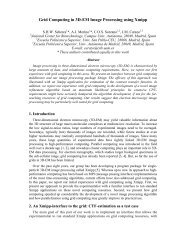
2 Your first 3D reconstruction in XMIPPRandom Conical Tilt reconstruction: To make a three-dimensional reconstruction ofelectron microscopy images one needs to combine projections from a large number of identicalobjects in different orientations. In this demo, the experimental projections have been obtainedby tilting the specimen inside the electron microscope following a collection geometry knownas random conical tilt (Radermacher, 1987). The only constraint imposed by this technique isthat the macromolecules must tend to lay onto the grid showing one or a few preferential views.Although this requirement may seem restrictive, it is fairly usual for biological molecules tointeract with the film support producing a collection of preferential views.The random azimuthal (in-plane) rotations make that the imaged macromolecules presentmany different views when we tilt the micrograph in the microscope. This set of views isformally equivalent to a conical tilt series with the cone angle equal to the tilt angle and theazimuthal angle set at random (Fig. 1). Two micrographs of each area of interest are taken. Thefirst one, which is tilted, provides the views used for the three-dimensional reconstruction, whilethe second one, which is not tilted, is employed to calculate the relative in-plane rotation anglesby cross-correlation techniques. Implicit to the method is the assumption that all projectionsderive from copies of identical three-dimensional objects, or that it is possible to classify themprior to the 3D-reconstruction.Therefore our task is to: select pairs of images in the different micrographs, align and classifythe untilted views, and make a 3D reconstruction with the tilted views.2.1 What are we working withIn this practical session we will work with images of the bacteriophage SPP1 hexameric helicaseG40P. Núñez-Ramírez et al. (2006). This protein interacts with the carbon support, resultingin a strong preference for frontal views, which makes it a suitable sample to be analysed byRandom Conical Tilt. From the literature we know that this protein is able to arrange into twodifferent states with different rotational symmetry, 3-fold and 6-fold. After hours of work in themicroscope (RCT data collection may be cumbersome!) you have pairs of tilted and untiltedmicrographs. That is, pairs of micrographs of the same area taken with different angles, one at0º and the other at 55º. We collected our data on photographic film, which was developed andsubsequently scanned yielding our micrographs in TIFF format. If you have downloaded andextracted the tarball mentioned on the first page of this document, you should have two of thesepairs (called pair1 and pair2) in the directory called my_experiment/Micrographs.2.2 Preprocess micrographsWe typically use a separate directory for each project/experiment (called the projectdir). Go tothe projectdir, in this case my_experiment:cd my_experimentto launch the GUI type:7

Figure 1: Illustration of the basic principle of the random conical tilting reconstruction scheme.(a) view of a specimen with randomly oriented particles lying flat in the plane of thespecimen; (b) tilted view of the same specimen. The projections of the specimen whichcan be extracted from the tilted image form a conical tilt series shown in (c), whichis equivalent to a tilt series of a single particle with random projection directions, alllying on the surface of a cone.8

Figure 2: Xmipp Protocols main menuxmipp_protocolsIf xmipp_protocols was never executed before in this directory, you will be asked+ Xmipp_protocols was never executed before in this directory.+ Make sure you run xmipp_protocols only in your project directory.+ You are in directory: /home/user/my_experiment+ Do you want to setup Xmipp protocols here? [y/n]:Just type y, and the master GUI will be launched (see Fig.2). The master GUI is the mainmenu of xmipp_protocols. Clicking on any of the available tasks will launch the GUI for thecorresponding protocol. To preprocess the tilted pair micrographs, click in the PreprocessMicrographs button. This will launch a pop-up window in which you can modify the relevantparameters and submit the job.Modify the parameters of the Preprocessing Micrographs according to the onesshown in Fig. 3. In the global parameters you must indicate where your micrograph files arestored, what extension is used, and where the protocol will write the output files. This protocolperforms several steps:1. Conversion of TIFF to raw format.9

2. Downsampling: we will reduce the size of the raw files 3 times in this example, i.e. wewill bin 3x3 pixels.3. CTF estimation. For this, we will need some information about the microscope (settings)you used. The parameters shown in Fig. 3 are the adequate ones for this experiment.Because CTF estimation takes approximately 10 minutes per micrograph, we have alreadyperformed this step for you, and the results are already in your directory structure.Therefore, give No for the option “Perform CTF estimation?”When you have completed the form, click on the Save & Execute button. A pop-up windowwill ask you is you want to use a job queuing system. This is useful on many large computerclusters, but if you are working on your own computer you will probably not have a queueingsystem, so answer No. The job will be executed immediately, and you may follow its output inthe terminal window from where you launched the GUI.When the protocol finishes, you will have your micrographs in the appropriate file format towork with. From the CTF estimation results (that were already calculated beforehand) you canobserve the aberrations that occur in the microscope during image formation. This may be usefulin order to discard bad micrographs.To observe the results of the CTF estimation press the Analyse Results button. This willlaunch a window as shown in Fig. 4. The CTFs of good micrographs typically have multipleconcentric rings, extending from the image center towards its edges. Bad micrographs may lackany rings or only have very few rings that hardly extend from the image center. A reasons todiscard micrographs may be the presence of strongly asymmetric rings (astigmatism) or ringsthat fade in a particular direction (drift), see Fig.5. Sometimes, the CTF estimation algorithmmay fail to find the rings even if they can be seen by eye. If this is the case, you may help thealgorithm to find the rings by clicking with the mouse right button and pressing “RecomputeCTF”. A graphical interface will help you to correctly identify the CTF.In our example the first and the third micrographs are tilted images. Tilted images typicallyhave an ellipse-shaped, very narrow CTF that is not very useful to indicate aberrations in theimage formation.This protocol has created a new directory named Preprocessing. Open a second terminaland look inside this directory with:ls PreprocessingHere you will find a directory for each of the micrographs, a selfile with all the active micrographs(called all_micrographs.sel), a selfile with the estimated CTFs (called all_ctfs.sel),and an exact copy of the executed script (called xmipp_protocol_preprocess_micrographs_backup.pywhich serves for backup purposes). In the case of Random Conical Tilt, we need another file thatcannot be created by the protocols. It is a selfile similar to all_micrographs.sel, but it hasthree columns, indicating which images are tilt pairs. This information will typically be storedin the notes you made during your microscopy session. We will call this file all_pairs.sel,and it looks like this:pair1_untilted/down3_pair1_untilted.raw pair1_tilted/down3_pair1_tilted.raw 110

Figure 3: Xmipp Preprocessing Micrographs GUI11

Figure 4: Output visualization of Xmipp Preprocessing Micrographs protocol. The all_ctfs.selwindow shows the CTF of all the micrographs. In this case is shown the CTFs of atilting pair. The first one is very poor defined and ellipse-shaped because it correspondsto the tilted images, whereas the second one is the CTF of the untilted micrograph.Figure 5: CTF of good, astigmatic and drift micrographs12

pair2_untilted/down3_pair2_untilted.raw pair2_tilted/down3_pair2_tilted.raw 1Where the first column contains the untilted image and the second column the tilted imageof each pair. The third column contains a normal selfile-like flag. Now, create your ownall_pairs.sel in the Preprocessing/ folder using you favorite text editor. For example,type:nedit all_pairs.sel &2.3 Manual Particle SelectionClose the Preprocessing GUI, go back to the main menu and click in the Manual ParticleSelection button. This will launch a window as shown in Fig. 6. Introduce the name ofthe micrograph selfile (in this case all_pairs.sel), and indicate that your micrographs aretilt pairs. Then, press Save & Execute, and a window as shown in Fig. 7 will appear.Click on Mark! to select particles in each pair of micrographs. This will launch an overviewwindow containing both micrographs and two zoom windows, one showing part of the untiltedmicrographs and the other showing part of the tilted micrograph (see Fig. 8).In order to select particles:• Arrange the zoom windows, such that the untilted micrograph is on the left side of yourscreen and the tilted one is on the right side. Perhaps you may want to enlarge the sizeof the zoom windows and make the overview window smaller (depending on the size ofyour screen). Just drag the window’s corners to do so.• Click with the mouse left button on the overview window for selecting the part of themicrograph in which you are interested (it will appear magnified in the respective zoomwindows). Use Ctrl+ and Ctrl- in the overview window to Zoom-in and Zoom-outrespectively.• Mark particles with the left mouse button in the zoom windows: First select a particlein the untilted image. This will suggest a corresponding point in the tilted micrograph.You may move its position by clicking the left mouse button on the desired position in thetilted image. You have now selected your first pair.• Initially the suggestions will be far off, but if you have correctly identified several pairs,they should improve. To explicitly recompute the transformation matrix select File->Saveangles (it is a good idea to do first File->Save coords, just in case something goeswrong). IMPORTANT: click a few pairs (at least four) before computing the transformationmatrix. Note that once the correct transformation has been found, the program shouldaccurately predict the position of the tilted particle after identifying the untilted one. Ifthis is not the case, you have probably included some incorrect pairs.• Click with the mouse right button over a selected particle in order to remove it or move it.13

Figure 6: Manual Particle Selection GUI• You can apply filters to the micrographs, so that you may see the particles better. Filtersare added into a queue, so whenever you change the visualized area, they are appliedagain. Select the menu filter in the overview window and add as many filters as you like.You can clean the filter queue, if you want to return to the original image.• By default particle are marked with a small circle. Some people like larger circles (adjustedto the size of their particles) or squares better. You may change this using theFile->Change mark radius and File->Change mark type menu options.• VERY IMPORTANT! Don’t forget to save the coords in BOTH micrographs before youexit. You can save the angles in one of the File menu of the two micrographs indistinctly.For many specimens, in particular for particles embedded in vitrified ice and of relativelysmall size (100-500 kDa), particle selection is a major obstacle for single particle analysis. Forthese cases, automated procedures usually perform much worse than manual picking. Therefore,a careful interactive selection of the particles, although being time-consuming, will generally14

Figure 7: GUI for Xmipp Manual Particle PickingFigure 8: Screen-shot of xmipp_micrograph_mark. The overview windows are placed at the topand the zoom windows at the bottom. The untilted micrograph is on the left and thetilted micrograph on the right15

Figure 9: A field of evenly distributed particles is shown on the left panel. On the right panelsthere are examples of micrographs with too many or heterogeneous particles. Barrepresents 50 nm.facilitate subsequent image processing steps. Some micrographs that were not discarded inthe CTF estimation, may be discarded at this stage, as a too high particle density or a strongheterogeneity in the particle population may hinder the selection process. Some examples aregiven in Fig. 9.By pressing the File->Save coords button in each window, the program saves a positionfile for each micrograph. Pressing File-> Save angles button saves a so-called angle file(with information about the transformation matrix) for each tilt pair. The position files are insidethe corresponding micrograph directory and the angle file is saved inside the correspondinguntilted micrograph directory. You can see them typingls */*.posls */*.angThe angles file looks like:# alpha_u alpha_t gamma75.783 74.6211 55.9613The tilt angle is the third value and should be (for this particular example) about 55º while thefirst two values (alpha_u and alpha_t) are the angles between the tilt axis and the y-axis for theuntilted and tilted image respectively. These values should be, for this particular example, about75º. As you select more and more particles the accuracy of these values should increase. (If youdo not get values close to these ones you have probably selected incorrect pairs.)2.4 Preprocess particlesClose the Manual Particle Selection GUI, and click on the Preprocess particlesbutton of the main menu to continue. This will launch the GUI of the next protocol that will allowyou to extract, normalize and correct the CTF-phase of your picked particles. Modify theparameters of the Preprocess Particle Protocol according to the parameters shownin Fig. 10.16

Figure 10: GUI of xmipp_protocol_preprocess_particles17

1. The protocol extracts the particles from the micrographs using the coordinates determinedin the previous step. You must indicate the name of the coordinate family (by defaultCommon) and the image dimension in pixels (in this case 80).2. The particles are normalized to have zero mean and a standard deviation of unity for thebackground pixels. You must define the background pixels as those outside a circle ofgiven radius (35 pixels in this case). Ramping background correction, black dust removaland white dust removal are optional flags to correct for ramping backgrounds and/or whiteor black outlier pixels (possibly dust particles).3. Finally, the protocol corrects the CTF-phase of your particles and/or sorts them based ongeneral statistics to identify outliers. For our example we do not perform these two finalsteps because they are not adequate for tilted images.Press the Analyse Results button to check the extracted and normalized images (see Fig.11). Play a little with the pop-up windows (right-click on the window to pop them). In particulartry Options->View Average and SD images. NOTE: before obtaining an averageimage you will need to select a set of images that you want to average (click on the desiredimages and press the space bar or double-click them with the left mouse button).This protocol has created a directory called Images/ in the projectdir, which contains all theextracted images sorted by micrographs. You can see that for each micrograph a sub-directoryhas been created by typing:cd ..ls -l Images/And you can see all individual particle files by typing:ls -l Images/*/*The protocol has also created two new selfiles in the projectdir (all_images_untilted.seland all_images_tilted.sel), which contain all the untilted and tilted images correspondingly.2.5 A much larger data setNow, we want to combine the information contained in all our (very noisy) particles to createan average image with high signal to noise ratio. However, we only can combine images thatare similar. That is, particles that represent different projection directions or that are projectionsfrom different 3D objects must be separated from each other before averaging. In order to solvethis problem, several 2D-classification tools have been developed in Xmipp. The most popularones are both based on maximum-likelihood principles and are called xmipp_kerdensomand xmipp_ml_align2d.Two micrographs do not provide enough particles for reliable classification and alignment.Therefore, we have previously executed the Preprocess Micrographs, Manual Particle18

Figure 11: Analyse results window of xmipp preprocess particle protocols. On the top is shownthe GUI with different options of visualization. In our case just click yes in the firstquestion. Below are shown the untilted and tilted images.19

Picking and Preprocess Particles using a much large number of micrograph pairs.of micrographs on the same sample used in the previous steps. To work with these data, closeall GUI windows, and go to the directory my_experiment_2/ by typing:cd ../my_experiment_2/Here you will find the same directory structure that you have already encountered in the previoussections.This experiment comprises approximately 3,000 image pairs. You may visualize themby typing:xmipp_show -sel all_images_untilted.sel all_images_tilted.sel &Note that these images have been windowed much smaller than before (50x50 pixels instead of80x80 pixels). This would not be normal practice, but has been done to speed up this demo.Launch the GUI from this new projectdir, by typing xmipp_protocols as before.2.6 Rotational Spectra ClassificationWe have important prior knowledge that the G40P helicase arranges into two different quaternarystructures with different rotational symmetry. This allows us to use the Rotational Power Spectraclassification protocol to separate the distinct states based on their symmetry.Press the Rotational Spectra Classification button to start the correspondingGUI, and introduce the parameters as shown in Figures 12 and 13. Upon pressing the Save &Execute button, this protocol will perform several steps:1. 2D alignment by cross-correlation of all particles. You must introduce some parameter forthe 2D alignment, like the number of iterations and the inner and outer radius (in pixels)that will be taken into account.2. Place the center of symmetry of the resulting average image in the center of the image.3. Calculate a rotational spectrum for each of the aligned images.4. Classify the rotational spectra by a neural network algorithm called kerdenSOM. Thisself-organizing map algorithm outputs a two-dimensional map of so-called code vectors(which are averages of multiple rotational spectra) that represent the distribution of thevariability in the data. The organization of the map is reflected in the fact that similar codevectors are close to each other, while different code vectors tend to be separated. It is up tothe user to identify distinct classes, each of which may comprehend several (neighboring)code vectors. The smoothness of the map is determined by so-called regularization parameters,and the algorithm proceeds from an initially high value (-reg0) to a lower value(-reg1) in a user-defined number of steps (-steps). Too high regularization values resultin too smooth output maps that do not explain the variability in the data, while too lowvalues yield maps that are not organized. Typically, one repeats this calculation multipletimes with different annealing parameters, in order to optimize the output map.20

Figure 12: xmipp Rotational Spectra Classification GUI. Part one.21

Figure 13: xmipp Rotational Spectra Classification GUI. Part two.22

Figure 14: Analyse results window of xmipp Rotational Spectra Classification.After the protocol has finished, press the Analyse Results button to visualize its output.The protocol will show you the selfile with the aligned images, the average image of this selfile,the individual rotational spectra of all the images and the KerdenSOM output map (see Fig. 14).The output map acts as a summary of the structural variability in the data, providing a convenienttool to interactively select different classes from large amounts of data. Each image in the outputmap (code vector) represents a group of the initial data items with similar characteristics. In theupper right corner of every code vector you can see a number, which is the number of inputspectra that were assigned to that code vector.You can save selfiles with the images belonging to selected codevector by clicking withthe right mouse button in the window. Select File->Save assigned images in aselfile and save the file wherever you want with the browser. Select Options in the samemenu to analyse your results in different ways. You can visualize the original images assignedto each code vector, or their corresponding average, modify the spectra visualization, change thespectra scale, etc.....Try to find the region of code vectors that have a maximum in the sixth harmonic, and theregion of code vectors that have a maximum at the third harmonic, and calculate the averageimage of the images assigned to these codevector.23

2.7 ML2D alignmentSince group selection may be a tricky step in Rotational Spectra Classification,we have selected the two types of frontal views of G40P for you: one of 6-fold symmetry and theother one of 3-fold symmetry. The selection files that contains these two groups of images arecalled simC6.sel and simC3.sel, and they are also stored in the projectdir. Now you willindependently align the images of one of these groups: simC6.sel. For this purpose we willuse the xmipp_ml_align2d program. This is a powerful and very general tool for simultaneousimage classification and alignment, but in this case we will only use it to align the images ofthe classes selected in the previous step. To run the corresponding protocol, click the ML2Dclassification button in the main menu. This will launch the ML2D classification GUI.Fill it according to the parameters shown in Fig. 15. Note that the number of classes to beused will just be one, as we will use this protocol only for alignment, and not for classification.Also make sure to select No in the question about the mirror transformation in the alignment,as selecting Yes will not work for the subsequent Random Conical Tilt experiment. If you usethis protocol on larger data sets (and with more than one class), you may need a considerableamount of CPU time. Therefore, you may want to use a multi-processor machine in such cases.In this practice you will use relatively few images (~3,000) and only one reference, so you willnot need to execute it in parallel.When the protocol has finished press the Analyse Results button and the visualize_ml2dwindow will pop-up (see Fig. 16). Mark Yes in all the questions and press Save & Execute.This will launch several windows.1. A window with the class averages of each iteration.2. A window with the class average of the last iteration.3. A plot indicating the fraction of particles that belongs of each class and the fraction onmirror inside each class. This information will not be very useful for our data, because weonly used 1 class and did not check for mirrors.4. Some plots illustrating the convergence behavior of the algorithm.2.8 Random Conical Tilt ReconstructionYou are now ready to perform your first 3D reconstruction! You have used the untilted imagesto classify and align the frontal views. Now you will use the in-plane rotations of the untiltedimages, together with the tilt angle determined during the manual picking process, to performa 3D reconstruction with the tilted images. We will do this using the data in simC6.sel andthereby calculate a 3D reconstruction for the 6-fold symmetric structure of G40P. To start thecorresponding protocol press the Random Conical Tilt button in the main menu window.Fill its GUI with the parameters shown in Fig. 17. You must indicate the selfiles with the untiltedand the tilted images, and the number(s) of the class(es) identified by ML2D. (If you would haveused ML2D to both align and classify your images, you could calculate a 3D reconstructionfor each of the classes. In our example we have only used one class, so just type 1). NOTE:As the frontal views of the particles have symmetry you can apply it in the reconstruction.24

Figure 15: ML2D classification GUI25

Figure 16: output ML2D classification GUI. This visualization protocol show the results ofml_align2d protocol.26

Press Show Expert Options and in Additional WBP Parameteres write -symc6. Then Press Save & Execute.The protocol consists of several steps:1. Prepare all images of the selected class(es), apply the alignment information in the headersof the untilted images to the headers of the tilted images and precenter the latter ones.2. Perform a 3D reconstruction with the centered tilted images. This option can be performedusing the faster option WBP or the potentially more accurate option ART.3. Low-pass filter the reconstructed volume(s).When the protocol finishes you can visualize its results by pressing the Analyse Resultsbutton. This GUI offers several options for visualization (see Fig. 18). You can check theuntilted aligned images, the average of this images and the different 3D reconstruction. In theupper part of the GUI you can select which of the maps you want to visualize, whereas in thelower part you must select the way in which you want to visualize them. You can visualize themap by slices along the three different axis (X,Y and Z) or by surface rendering in case you haveUCSF Chimera installed in your machine (see Fig. 19).NOTE: In order to speed up the different steps involved in this demo we have masked verytightly the experimental data. In fact, they are saved as 50x50 pixels images instead of the80x80 pixels images used by Núñez-Ramírez et al. (2006). The side effect of this policy is theappearance of artifacts at the volume borders.2.9 KerdenSOM ClassificationNow we will make a little excursion to have a more detailed look at the KerdenSOM algorithm.We will use it to look for additional heterogeneity inside the other class of G40P (simC3.sel).First, you will again need to align the images of this selfile, otherwise the main heterogeneitythat you would find would be in shift and rotation of the images. To align the images you canagain use the ML2D classification protocol (following the instructions as given in section 2.7).Once the images are aligned, press the KerdenSOM classification button in the mainmenu, and fill out the form as shown in Fig. 20. Introduce correctly the directory where youhave perform the alignment by xmipp_ml_align2d, and indicate which class of this run you wantto use (in this case there is only one class!).The protocol comprises two steps:1. Design a mask that defines the region of interest in the average image of all particles. Thisprocess is user-interactive and will launch a graphical tool that will allow you to designmasks of different shape or size. Play with this tool until you have a suitable mask forthese data. Click the right mouse button in the window to pop-up a menu. In the Help->Help! you will find instruction on how to change the size and position of your mask. The27

Figure 17: Random Conical Tilt GUI.28

Figure 18: Output Random Conical Tilt GUI. It is shown the visualization GUI and three of theseveral output window that you can visualize: selfile with the untilted aligned images,the average image of this images and the 3D reconstruction showed by slices in theZ-axis.29

Figure 19: Chimera visualization of the Random Concial Tilt output mapMask types menu allows to change the shape of the mask. We recommend a circularcrown mask that encapsulates the particle. Then just quit the program using the Quitoption in the pop-up menu and the protocol will continue automatically.2. Compute a kerdenSOMAs described in more detail in section 2.6, the output of the algorithm (see Fig. 21) is a collectionof images (code vectors), which represent the main features of variability in our sample. You canselected code vectors by double clicking the left-mouse button or by pressing the space bar. Youcan save selfiles with images belonging to the selected codevectors by clicking with the rightmouse button in the window. Select File->Save assigned images in a selfileand save the file wherever you want with the browser. Select Options in the same menu tocalculate the average image and standard deviation of the images assigned to the selected codevectors.The relevant question to answer with this SOM is: “is there any remaining structural variability?”.2.10 Want more?We have followed a particular data processing work flow that was suitable for the particular casein this demo (RCT data of a molecule that always falls in the same orientation on the grid andthat shows differences in rotational symmetry that may be used for its classification). If you30

Figure 20: KerdenSOM Classification GUI31

Figure 21: Output KerdenSOM Classification protocol GUI. In the lower part is shown the KerdenSOMmap in which there are codevector that represent a group of individual imageswith similar characteristics. The two insets are the average images of the groupof images assigned to the two codevector highlighted32

would like to continue with these data, we suggest you repeat the last two protocols with theother symmetry architecture of G40P. That is, find the 3D reconstruction of the 3-fold structureof G40P (simC3.sel) by Random Conical Tilt and try to find remaining heterogeneities inthe 6-fold group of G40P (simC6.sel) using KerdenSOM. Remember that you have alreadyaligned both classes using the ML2D classification protocol, so you may skip that part. Note thatyou could also use the kerdenSOM to obtain a smaller (more homogeneous) class and performa RCT reconstruction for those particles.33

3 Concluding remarksThe Preprocessing stage is common for most data sets, but the work flow through the subsequentprotocols highly depends on the questions you want to answer. An overview of the possibleworkflows is given in Figure 22. Note that protocols indicated in orange may be executed inparallel on multi-processor (super-) computers. A list of some of the most popular work flows isgiven below.• In this demo we have performed RCT reconstruction of particles that have a strong preferentialtop view and that can be classified based on their rotational symmetry. We haveperformed this work flow: [Rotational Spectra Classification -> ML2D classification ->RCT reconstruction].• In the more general case of RCT reconstruction, particles fall in many different orientationson the grid and rotational spectra may not be used for classification. In this case onewould simultaneously align and classify the distinct projection directions using ML2Dclassification (with multiple classes), and then perform a RCT 3D reconstruction for eachof the classes separately: [ML2D classification -> RCT reconstruction]. In theory, thisshould give several different rotated versions of the same 3D structure (except for missingcone artefacts, flattening etc.). Currently, we do not have a standardized protocol to alignthese 3D volumes, but you may use the stand-alone program xmipp_align_volumesfor that.• 2D analysis of structurally heterogeneous data (i.e. data comprising projections of differentproteins/complexes, exhibiting different projection directions or distinct conformations)is generally performed using [ML2D classification]. In many cases, this alreadyresults in a satisfactory separation of the (2D) structural heterogeneity. However, one mayalways perform a check for additional variability using a subsequent kerdenSOM classification.[ML2D classification -> kerdenSOM classification]. In particular, the ability touse a focused mask has been very useful in the past to classify small changes that occur ina specific, localized areas (we did this in section 2.9).• Once we have an initial 3D reconstruction (obtained through RCT or by other means),we may choose to separate structural heterogeneity (e.g. in the form of distinct conformations)through [ML3D classification]. The resulting classes (which are hopefullyhomogeneous) may then be refined separately as explained in the next step.• If we have an initial 3D reconstruction and our data are structurally homogeneous, thenwe may refine the initial 3D map using either [Projection matching refinement] or [Multiresolutionrefinement].Finally, please remember that our funding depends on your citations to our work. Therefore, ifXMIPP has been useful in your research, please cite our papers. A detailed list of relevantreferences may be found on the XMIPP Wiki ListOfReferences.Have fun!!The Xmipp team34

Figure 22: Flow chart of possible data processing strategies35

ReferencesMarabini, R., Masegosa, I. M., M. C. San Martín, S. M., Fernández, J. J., L. G. de la Fraga, C. V.,and Carazo, J. M. (1996). Xmipp: An image processing package for electron microscopy. J.Struct. Biol., 116:237–240.Núñez-Ramírez, R., Robledo, Y., Mesa, P., Ayora, S., Alonso, J. C., Carazo, J. M., and Donate,L. E. (2006). Quaternary polymorphism of replicative helicase g40p: Structural mapping anddomain rearrangement. J Mol Biol.Radermacher, M. (1987). Three-dimensional reconstruction from a single-exposure, randomconical tilt series applied to the 50s ribosomal subunit of escherichia coli. J.Microsc, 146:113–136.Sorzano, C. O. S., Marabini, R., Carazo, J. M., Velázquez-Muriel, J., Bilbao-Castro, J. R.,Fernández, J. J., and Pascual-Montano, A. (2004). Xmipp: A new generation of the opensourceimage processing package for electron microscopy. J. Struct. Biol., 148:194–204.36