An Introduction to Plasma Physics and its Space Applications
An Introduction to Plasma Physics and its Space Applications
An Introduction to Plasma Physics and its Space Applications

Create successful ePaper yourself
Turn your PDF publications into a flip-book with our unique Google optimized e-Paper software.
<strong>An</strong> <strong>Introduction</strong> <strong>to</strong> <strong>Plasma</strong> <strong>Physics</strong><br />
<strong>and</strong> <strong>its</strong> <strong>Space</strong> <strong>Applications</strong><br />
Dr. L. Conde<br />
Department of Applied <strong>Physics</strong><br />
ETS Ingenieros Aeronáuticos<br />
Universidad Politécnica de Madrid<br />
March 5, 2014
These notes are not intended <strong>to</strong> replace any of the excellent textbooks (as Refs.<br />
[1, 2, 3, 4, 7] ) cited in the bibliography, but <strong>to</strong> free <strong>to</strong> those attending this course<br />
of the thankless task of taking notes. The reader will find that are a very preliminary<br />
version that is far from being concluded. Some citations in the text <strong>to</strong> the<br />
references are still incomplete <strong>and</strong> the english requires of a major revision. I am<br />
responsible for all errors <strong>and</strong>/or omissions.<br />
I <strong>to</strong>ok the liberty of borrowing some original figures <strong>and</strong> graphs from cited references<br />
<strong>to</strong> illustrate certain points. Also <strong>to</strong> allow <strong>to</strong> these students the calculations of<br />
relevant quantities using actual experimental data. Additionally, I also make use<br />
of two pho<strong>to</strong>graphs of a solar eclipse from NASA that I found in the Wikipedia<br />
article on the solar chromosphere. My thanks <strong>to</strong> the authors for sharing these<br />
materials as well as for their unintentional collaboration.<br />
L. Conde
Contents<br />
1 <strong>Introduction</strong> 1<br />
1.1 Ionized gases <strong>and</strong> plasmas . . . . . . . . . . . . . . . . . . . . . . . . . . . . . . 1<br />
1.2 Properties of plasmas . . . . . . . . . . . . . . . . . . . . . . . . . . . . . . . . . 2<br />
1.3 The ideal Maxwellian plasma . . . . . . . . . . . . . . . . . . . . . . . . . . . . 2<br />
1.4 The Maxwellian plasma under an external electric field . . . . . . . . . . . . . . 5<br />
1.5 The plasma parameters . . . . . . . . . . . . . . . . . . . . . . . . . . . . . . . 7<br />
1.5.1 The Debye length . . . . . . . . . . . . . . . . . . . . . . . . . . . . . . . 7<br />
1.5.2 The plasma frequency . . . . . . . . . . . . . . . . . . . . . . . . . . . . 9<br />
1.5.3 The plasma <strong>and</strong> coupling parameters . . . . . . . . . . . . . . . . . . . . 10<br />
1.6 Magnetized plasmas . . . . . . . . . . . . . . . . . . . . . . . . . . . . . . . . . 12<br />
2 The plasmas in space <strong>and</strong> in the labora<strong>to</strong>ry. 15<br />
2.1 The plasma state of condensed matter . . . . . . . . . . . . . . . . . . . . . . . 15<br />
2.2 <strong>Plasma</strong>s in astrophysics . . . . . . . . . . . . . . . . . . . . . . . . . . . . . . . 17<br />
2.3 Geophysical plasmas . . . . . . . . . . . . . . . . . . . . . . . . . . . . . . . . . 18<br />
2.4 Labora<strong>to</strong>ry plasmas . . . . . . . . . . . . . . . . . . . . . . . . . . . . . . . . . . 19<br />
3 Bibliography, texbooks <strong>and</strong> references 22<br />
3.1 Textbooks . . . . . . . . . . . . . . . . . . . . . . . . . . . . . . . . . . . . . . . 22<br />
3.2 Bibliography on space plasmas . . . . . . . . . . . . . . . . . . . . . . . . . . . 23<br />
3.3 References on gas discharge physics . . . . . . . . . . . . . . . . . . . . . . . . . 23<br />
3.4 Additional material . . . . . . . . . . . . . . . . . . . . . . . . . . . . . . . . . . 23<br />
4 The elementary processes <strong>and</strong> the plasma equilibrium 25<br />
i
Escuela de Ingeniería Aeronáutica y del Espacio<br />
Universidad Politécnica de Madrid<br />
4.1 The collision cross section . . . . . . . . . . . . . . . . . . . . . . . . . . . . . . 26<br />
4.2 The <strong>to</strong>tal <strong>and</strong> differential cross sections. . . . . . . . . . . . . . . . . . . . . . . 27<br />
4.3 Cross section <strong>and</strong> impact parameter . . . . . . . . . . . . . . . . . . . . . . . . 29<br />
4.4 The a<strong>to</strong>mic collisions in plasmas . . . . . . . . . . . . . . . . . . . . . . . . . . 30<br />
4.4.1 The electron collisions with neutrals . . . . . . . . . . . . . . . . . . . . 32<br />
4.4.1.1 The elastic collisions . . . . . . . . . . . . . . . . . . . . . . . . 32<br />
4.4.1.2 Inelastic collisions . . . . . . . . . . . . . . . . . . . . . . . . . 32<br />
4.4.2 Ion collisions with neutrals . . . . . . . . . . . . . . . . . . . . . . . . . 38<br />
4.4.3 Pho<strong>to</strong>processes . . . . . . . . . . . . . . . . . . . . . . . . . . . . . . . . 38<br />
4.4.4 The collisions of charged particles . . . . . . . . . . . . . . . . . . . . . . 41<br />
4.4.4.1 The electron <strong>and</strong> ion recombination . . . . . . . . . . . . . . . 41<br />
4.4.4.2 The Coulomb collisions . . . . . . . . . . . . . . . . . . . . . . 42<br />
4.5 Numerical estimates . . . . . . . . . . . . . . . . . . . . . . . . . . . . . . . . . 42<br />
4.6 The equilibrium states of a plasma . . . . . . . . . . . . . . . . . . . . . . . . . 44<br />
4.6.1 Multithermal equilibrium . . . . . . . . . . . . . . . . . . . . . . . . . . 45<br />
4.6.2 The local equilibrium . . . . . . . . . . . . . . . . . . . . . . . . . . . . . 46<br />
5 The physical models for plasmas 47<br />
5.1 The kinetic description of plasmas . . . . . . . . . . . . . . . . . . . . . . . . . 49<br />
5.1.1 The Boltzmann collision integral . . . . . . . . . . . . . . . . . . . . . . 53<br />
5.2 The transport fluid equations . . . . . . . . . . . . . . . . . . . . . . . . . . . . 56<br />
5.2.1 The averages of the distribution function. . . . . . . . . . . . . . . . . . 57<br />
5.2.2 The equation of continuity. . . . . . . . . . . . . . . . . . . . . . . . . . 60<br />
5.2.3 The momentum transport equation. . . . . . . . . . . . . . . . . . . . . 61<br />
5.2.4 The energy transport equation. . . . . . . . . . . . . . . . . . . . . . . . 63<br />
5.2.5 The closure of the fluid transport equations . . . . . . . . . . . . . . . . 64<br />
5.2.6 The friction coefficients . . . . . . . . . . . . . . . . . . . . . . . . . . . 66<br />
5.2.6.1 Elastic collisions. . . . . . . . . . . . . . . . . . . . . . . . . . 68<br />
5.2.6.2 Ionizing collisions. . . . . . . . . . . . . . . . . . . . . . . . . 69<br />
6 The boundaries of plasmas: the plasma sheaths. 70<br />
6.1 <strong>Introduction</strong>. . . . . . . . . . . . . . . . . . . . . . . . . . . . . . . . . . . . . . 70<br />
6.2 The collisionless electrostatic plasma sheath. . . . . . . . . . . . . . . . . . . . . 70<br />
6.2.1 Bohm Criterion. . . . . . . . . . . . . . . . . . . . . . . . . . . . . . . . 72<br />
6.2.2 Child-Langmuir current. . . . . . . . . . . . . . . . . . . . . . . . . . . . 74<br />
ii
1<br />
<strong>Introduction</strong><br />
1.1 Ionized gases <strong>and</strong> plasmas<br />
In essence, a plasma is a gas where a fraction of <strong>its</strong> a<strong>to</strong>ms or molecules are ionized. This<br />
mixture of free electrons, ions <strong>and</strong> neutral gas a<strong>to</strong>ms (α = i, e, a) is denominated a fully<br />
ionized plasma when all neutral gas a<strong>to</strong>ms are ionized <strong>and</strong> partially ionized otherwise.<br />
In the thermodynamic equilibrium of a gas <strong>its</strong> a<strong>to</strong>ms have a Maxwell Boltzmann velocity<br />
distribution determined by the temperature T of the system. This latter is usually expressed<br />
in un<strong>its</strong> of energy k B T in <strong>Plasma</strong> <strong>Physics</strong>. In these conditions, the average velocity of these<br />
neutral particles is,<br />
V a,T h =<br />
( 8 kB T<br />
π m a<br />
) 1/2<br />
Then, for growing temperatures the kinetic energy of an increasing fraction of the a<strong>to</strong>ms lies<br />
over the ionization threshold E I of the the neutral gas. The collisions of these energetic<br />
particles may produce the ionization of a neutral gas a<strong>to</strong>m. Consequently, the degree of<br />
ionization <strong>and</strong> the thermal temperature of the neutral gas are closely related magnitudes.<br />
This is why the plasma state is frequently associated with high temperature gases, because<br />
they reach an equilibrium state where <strong>its</strong> a<strong>to</strong>ms become fully or partially ionized.<br />
Nevertheless, the detailed derivation of the explicit relation between the equilibrium temperature<br />
T <strong>and</strong> the ionization degree of a gas will not be carried out here. The classical result<br />
is the Saha equation,<br />
n e n i<br />
n a<br />
≃ 2.4 × 10 21 T 3/2 exp(−E I /k b T )<br />
where n e , n i <strong>and</strong> n a respectively are the number of electrons, ions <strong>and</strong> neutral a<strong>to</strong>ms per<br />
volume unit.<br />
However, the above expression predicts very low ionization degrees even for high temperatures.<br />
Therefore, the thermodinamic equilibrium of partially ionized gases only take place<br />
for extremely high temperatures. This restrictive condition is seldom found in nature <strong>and</strong><br />
1
Escuela de Ingeniería Aeronáutica y del Espacio<br />
Universidad Politécnica de Madrid<br />
most plasmas in nature <strong>and</strong> in the labora<strong>to</strong>ry are physical systems far from thermodynamic<br />
equilibrium. The energy is lost by different physical mechanisms as the emission of visible<br />
light, electric current transport, ...etc. These energy losses are sustained by external energy<br />
contributions as external radiation, electromagnetic fields, ... etc.<br />
1.2 Properties of plasmas<br />
More precisely, the plasma state of matter 1 can be defined as the mixture of positively charged<br />
ions, electrons <strong>and</strong> neutral a<strong>to</strong>ms which constitutes a macroscopic electrically neutral medium<br />
that responds <strong>to</strong> the electric <strong>and</strong> magnetic fields in a collective mode. These physical systems<br />
have the following general properties:<br />
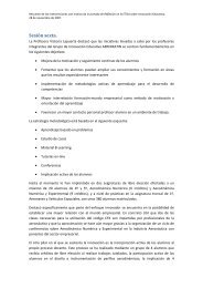
g(E)<br />
• The charged particles interact through long distance electromagnetic forces <strong>and</strong> the<br />
number of positive <strong>and</strong> negative charges is equal, so that the medium is electrically<br />
neutral.<br />
• In the following, the electromagnetic interaction will be regarded as instantaneous, we<br />
will not cope with relativistic effects. The electromagnetic forces experienced by charged<br />
particles can be approximated by the Lorentz force.<br />
0.6<br />
0.4<br />
0.2<br />
0.0<br />
k B T = 1.0 eV<br />
k B T = 1.5 eV<br />
k B T = 2.0 eV<br />
0 4 8<br />
Energy (eV)<br />
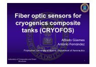
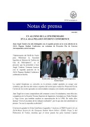
Figure 1.1: The Maxwell Boltzmann<br />
energy distribution function g(E) for<br />
different temperatures k B T .<br />
A particular feature of plasmas is the collective response<br />
<strong>to</strong> external perturbations. In ordinary gases,<br />
the fluctuations of the pressure, energy, ...etc. are<br />
propagated by collisions between the neutral a<strong>to</strong>ms.<br />
This requires the close approach of the colliding particles.<br />
In addition <strong>to</strong> this short scale interaction, the<br />
long range electromagnetic forces in plasmas also propagate<br />
the perturbations affecting the motion of large<br />
number of ions <strong>and</strong> electrons. Therefore, the response<br />
<strong>to</strong> the perturbations of electromagnetic fields is collective,<br />
involving huge numbers of charged particles.<br />
Obviously, the multicomponent plasmas are constituted<br />
by a mixture of different kinds of a<strong>to</strong>ms. Additionally,<br />
the dusty plasmas also include charged solid<br />
microparticles. The large mass <strong>and</strong> electric charge acquired<br />
by these dust grains introduce new properties<br />
in these physical systems.<br />
For simplicity, we will limit in the following <strong>to</strong> one component classical plasmas composed<br />
by electrons <strong>and</strong> single charged ions.<br />
1.3 The ideal Maxwellian plasma<br />
Let us briefly recall some properties of the equilibrium Maxwell Boltzmann energy distribution<br />
for a neutral gas composed by a single kind of a<strong>to</strong>ms with mass m. It may be shown that this<br />
1 Note that such statement is frequently, used but is somehow misleading because the different states of<br />
condensed matter may be found in thermodynamic equilibrium.<br />
2
Curso 2013-2014 <strong>An</strong> introduction <strong>to</strong> <strong>Plasma</strong> <strong>Physics</strong>, ...<br />
distribution describes a gas in the thermodynamic equilibrium state at the temperature k B T .<br />
This distribution may be expressed as,<br />
m<br />
f(v) = (<br />
2πk B T )3/2 exp (− m v2<br />
2k B T ) (1.1)<br />
where v is the particle velocity. This velocity distribution only depends on v = |v| <strong>and</strong> the<br />
integral over all possible velocities gives,<br />
∫ +∞<br />
−∞<br />
f(v) dv =<br />
∫ +∞<br />
−∞<br />
f(v) (4π v 2 ) dv = 1<br />
In the equilibrium the number n o number of particles by unit volume is uniform <strong>and</strong>,<br />
∫ +∞<br />
−∞<br />
n o f(v) dv = n o<br />
Therefore dn = n o f(v) dv represents the density of particles with velocities between v <strong>and</strong><br />
v + d v. Equivalently, dP = f(v) dv is the probability of finding a particle with this velocity<br />
range by volume unit. Using the particle kinetic energy E = mv 2 /2 in the Eq. (1.1) <strong>and</strong><br />
integrating,<br />
∫ ∞<br />
0<br />
g(E) dE = 1 where, g(E) = 2 √ π<br />
√<br />
E<br />
(k B T ) 3/2 e−E/k BT<br />
(1.2)<br />
This energy distribution function g(E) is equivalent <strong>to</strong> f(v) in Eq. (1.1) <strong>and</strong> is represented<br />
in Fig. (1.1) for different temperatures k B T .<br />
As is evidenced in Fig. (1.1), the distribution becomes broader as the temperature increases<br />
<strong>and</strong> dn = n o g(E) dE represents the number of particles with kinetic energy between E <strong>and</strong><br />
E +dE. The broadening of Fig. (1.1) shows the increment in the number of energetic particles<br />
for increasing k B T .<br />
The physical magnitudes are obtained from the equilibrium distributions (1.1) <strong>and</strong> (1.2)<br />
as averages. The kinetic energy by particle is e i is,<br />
e i =< 1 2 mv2 >= 1 ∫ +∞<br />
f(v) ( 1 n o 2 mv2 ) dv = 1 ∫ ∞<br />
f(v) ( 1 n o 2 mv2 ) (4π v 2 ) dv = 3 2 k BT<br />
−∞<br />
<strong>and</strong> the internal energy of this monoa<strong>to</strong>mic gas is therefore E i = n o e i . Note in Fig. (1.1) hat<br />
while <strong>its</strong> maximum value is e max = k B T/2 the average kinetic energy by particle e c = 3 k B T/2<br />
is slightly higher.<br />
Other different average speeds are currently defined for the Maxwell Boltzmann distribution<br />
function. As the thermal velocity, v T h = √ 2k B T/m which may be used <strong>to</strong> rewrite Eq.<br />
(1.1) as,<br />
1<br />
f(v) = (<br />
π 3/2 vT 3 ) exp ( −v 2 /v 2 )<br />
T h<br />
h<br />
0<br />
3
Escuela de Ingeniería Aeronáutica y del Espacio<br />
Universidad Politécnica de Madrid<br />
The average speed is defined as ¯v =< |v| > <strong>and</strong>,<br />
¯v =< √ v · v >=<br />
∫ +∞<br />
0<br />
(<br />
f(v) v (4π v 2 8kB T<br />
) dv =<br />
π m<br />
(1.3)<br />
Since the Maxwell Boltzmann distribution only depends<br />
on |v| the average along a fixed direction,<br />
) 1/2<br />
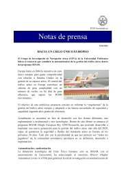
φ (x)<br />
Ions<br />
<strong>Plasma</strong><br />
Electrons<br />
< v x >=< v y >=< v z >= 0<br />
This reflects the fact that in the equilibrium of an ideal<br />
gas there is no privileged direction for the particle<br />
speed. On the contrary, the average,<br />
Distance<br />
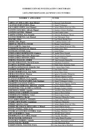
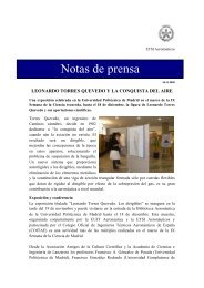
Figure 1.2: Polarization of a plasma<br />
cloud under an external electric field<br />
E = −∇φ(x).<br />
X<br />
< |v x | >=<br />
( 2kB T<br />
π m<br />
) 1/2<br />
= 1 2 ¯v<br />
represents the average speed of particles crossing an imaginary plane drawn perpendicular <strong>to</strong><br />
the x direction within the gas bulk. The r<strong>and</strong>om flux of particles Γ crossing such surface is,<br />
Γ = 1 2 n < |v x| >= 1 4 n o ¯v<br />
where the fac<strong>to</strong>r 1/2 accounts for the two possible directions of incident particles.<br />
As for neutral gases, the Maxwell Boltzmann distributions (1.2) <strong>and</strong> (1.2) may be used <strong>to</strong><br />
describe the thermodynamic equilibrium state of an ideal plasma 2 . This physical situation is<br />
roughly characterized by:<br />
1. The energy distribution function of each specie (ions electrons <strong>and</strong> neutral a<strong>to</strong>ms) is a<br />
Maxwellian with a common kinetic temperature k B T for all species. This latter is also<br />
the temperature of the thermodynamic equilibrium state of the plasma.<br />
2. In order <strong>to</strong> preserve the bulk electric charge neutrality, the ion <strong>and</strong> electron volume densities<br />
n io ≃ n eo = n o are equals. This property is denominated the plasma quasineutrality<br />
<strong>and</strong> results in a negligible electric field E ≃ 0 in the plasma bulk.<br />
3. The plasma potential φ(r) ≃ φ o is therefore uniform in space, so that no currents nor<br />
transport of particles takes place in a Maxwellian plasma.<br />
4. The kinetic temperatures k B T are also uniform in space <strong>and</strong> are usually expressed in<br />
energy un<strong>its</strong>. They are currently measured in electron volts (eV ) in <strong>Plasma</strong> <strong>Physics</strong><br />
because of the large energies involved (1 eV = 11,605 K).<br />
A rising temperature increments the average kinetic energy <strong>and</strong> the energy distribution<br />
function becomes wider as shown in Fig. (1.1). The limit k B T = 0 for a cold plasma corre-<br />
2 The use of the term ideal should be remarked. The requisites for the thermodynamic equilibrium of a plasma<br />
are extremely restrictive <strong>and</strong> plasmas essentially in stationary states far from the thermodynamic equilibrium.<br />
4
Curso 2013-2014 <strong>An</strong> introduction <strong>to</strong> <strong>Plasma</strong> <strong>Physics</strong>, ...<br />
sponds <strong>to</strong> a monoenergetic particle population <strong>and</strong> <strong>its</strong> energy distribution could be approximated<br />
by a Dirac delta function. In this case, all particles have exactly the same velocity <strong>and</strong><br />
there is no energy spread around a mean value, contrary <strong>to</strong> the case k B T ≠ 0 corresponding<br />
<strong>to</strong> a finite temperature plasma.<br />
Therefore, in the ideal plasma in thermodynamic equilibrium the kinetic temperature k B T<br />
is the same for all species, while the electron <strong>and</strong> ion thermal speeds differ,<br />
v e,T h = √ 2 k B T/m e <strong>and</strong>, v i,T h = √ √<br />
2 k B T/m i = v e,T h me /m i<br />
The ion velocity v i,T h is lower than the electron thermal speed, because of their different<br />
masses. As we will see later, when the plasma is far from thermodinamic equilibrium the<br />
temperatures of the species k B T e are also different <strong>and</strong> is frequently found that k B T i ≪ k B T e .<br />
1.4 The Maxwellian plasma under an external electric field<br />
In order <strong>to</strong> introduce some basic properties<br />
we will consider an ideal, fully ionized<br />
plasma of ion <strong>and</strong> electrons. The initial<br />
charged particle densities n io , n eo <strong>and</strong><br />
temperature k B T are constant in time <strong>and</strong><br />
uniform in space.<br />
This initial equilibrium is perturbed by<br />
an external 3 , one dimensional electric field<br />
E = −∇φ(r). After reaching an stationary<br />
state, both charged species separate as<br />
shown in Fig. (1.2). The electrons (blue<br />
dots) are attracted <strong>to</strong>wards the high potential<br />
side whereas the ions (red dots) move on<br />
the opposite direction.<br />
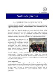
Particle densities n α (x) / n αo<br />
2.0<br />
1.0<br />
0.0<br />
2.0 eV<br />
5.0 eV<br />
n e (x)<br />
k B T = 1.0 eV<br />
k B T = 1.0 eV<br />
ϕ(x)<br />
–1.0 –0.5 0.0 0.5 1.0<br />
Distance<br />
5.0 eV<br />
2.0 eV<br />
n i (x)<br />
Electric potential<br />
profile<br />
The disturbance introduced by the electric<br />
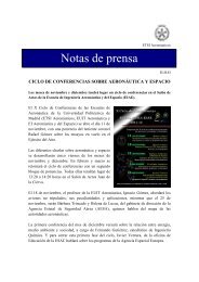
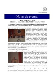
potential profile φ(x) brings the plasma Figure 1.3: The applied electric potential φ(x),<br />
out of equilibrium <strong>and</strong> produces a one dimensional<br />
spatial profile of the electron n e (x) tion of the distance X.<br />
electron n e (x) <strong>and</strong> ion n i (x) densities as a func-<br />
<strong>and</strong> ion n i (x) densities. However, the strength of this external electric field is not <strong>to</strong>o strong,<br />
so that the charge separation along the plasma potential profile φ(x) is not complete. The<br />
electrostatic energy (∼ e φ(x)) is of the same order than the thermal energy (∼ k B T ) of ions<br />
<strong>and</strong> electrons <strong>and</strong> therefore both charge species coexist along the spatial profile φ(x).<br />
In these conditions the energy of each charged particle (α = i, e) is E α = m α v 2 /2 +q α φ(r)<br />
where q α = ±e <strong>and</strong> the Maxwellian energy distribution (Eq. 1.1) for each specie is,<br />
m α<br />
f α (v) = (<br />
2πk B T )1/2 exp<br />
Integrating over v α we obtain for ions,<br />
(<br />
− m α vα 2 )<br />
+ 2 q α φ(r)<br />
2k B T<br />
2.0<br />
1.0<br />
0.0<br />
Electric potential ϕ(x) (Volts)<br />
(1.4)<br />
3 This point is emphasized because this potential profile φ(x) is essentially produced by an external electric<br />
field, the contribution of charged particles is neglected.<br />
5
Escuela de Ingeniería Aeronáutica y del Espacio<br />
Universidad Politécnica de Madrid<br />
n i (x) = n io exp (− e φ(x)<br />
k B T ) (1.5)<br />
<strong>and</strong> for electrons,<br />
n e (x) = n eo exp ( e φ(x)<br />
k B T ) (1.6)<br />
In Fig. (1.3) are represented the plasma potential profile φ(x) (black solid line, right axis<br />
between -0.5 V <strong>and</strong> 1.5 V) <strong>and</strong> the corresponding densities of charged particles given by Eqs.<br />
(1.5) <strong>and</strong> (1.6), which reproduces the situation depicted in the scheme of Fig. (1.2).<br />
Since the values for φ(x) in Fig. (1.3) are moderate <strong>and</strong> similar <strong>to</strong> the plasma temperatures<br />
k B T ≃ 1-5 eV both charged species coexist in the range −1 ≤ x ≤ 1. The electron densities<br />
n e (x)(blue curves) increase for φ(x) < 0 (x < 0) when k B T grows <strong>and</strong> the same effect takes<br />
place for ions for φ(x) > 0 (x > 0).<br />
The electron densities n e (x) (blue curves) dominate for positive potentials (x > 0 <strong>and</strong><br />
φ(x) > 0) where ions are rejected whereas the opposite situation occurs for x < 0 where<br />
φ(x) < 0. At the point x = 0 the electric potential is null <strong>and</strong> the Eqs. (1.5) <strong>and</strong> (1.6)<br />
recover the equilibrium particle densities n eo = n io . In the figure (1.3) the spatial profiles for<br />
electrons <strong>and</strong> ions are not equivalent with respect <strong>to</strong> the vertical dashed line at x = 0 because<br />
the electric potential φ(x) is asymmetric.<br />
This increment of n e (x) for x < 0 (equivalently, n i (x) for x > 0) with the plasma temperature<br />
takes place because the Maxwellian electron (ion) energy distribution g e (E) (for ions<br />
g i (E)) becomes broader when k B T grows as shows the Fig. (1.1). For points close <strong>to</strong> x ≃ −0.5<br />
an increasing fraction of electrons have enough thermal energy <strong>to</strong> overcome the electrostatic<br />
potential energy e φ(x). The situation is similar for the ions at the point x ≃ 0.5.<br />
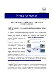
n e<br />
n i<br />
E X E X<br />
+<br />
δ X<br />
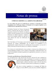
Figure 1.4: The space fluctuation<br />
of the electron n e (x)<br />
<strong>and</strong> ion n i (x) densities produce<br />
a local electric field E x<br />
in the plasma.<br />
In the case of a cold plasma k B T ≃ 0 the charged particles<br />
have no thermal energy. They only move under the external<br />
electric field <strong>and</strong> both species separate in space. On the contrary,<br />
in a finite temperature plasma (k B T >0) <strong>and</strong> despite the<br />
charged particle α is rejected when q α φ(x) < 0, a fraction of<br />
them have thermal energy enough <strong>to</strong> jump the electric potential<br />
barrier. For finite temperatures the thermal energy competes<br />
with the magnitude of the electrostatic energy of the plasma<br />
electric potential profile.<br />
The thermal energy of charged particles considered in Eqs.<br />
(1.5) <strong>and</strong> (1.6) brings a relevant property of plasmas: Their<br />
ability <strong>to</strong> shield out the electromagnetic perturbations. When<br />
moderate electric fields are externally applied or low amplitude<br />
electric fluctuations occur in the plasma bulk, the thermal motion<br />
of charged particles shields the perturbations as in Fig.<br />
6
Curso 2013-2014 <strong>An</strong> introduction <strong>to</strong> <strong>Plasma</strong> <strong>Physics</strong>, ...<br />
(1.3) by electrons <strong>and</strong> ions with energy enough <strong>to</strong> overcome the potential barrier.<br />
1.5 The plasma parameters<br />
The physical description of a plasma requires of a characteristic time <strong>and</strong> length scales <strong>and</strong><br />
additionally, a minimum number of charged particles by unit volume. These parameters are<br />
related with the attenuation of the small amplitude fluctuations of the equilibrium state of<br />
the plasma.<br />
As indicated in Fig. (1.4), when an small charge fluctuation δq = e δ(n i − δn e ) occurs<br />
in a plasma in equilibrium, the local positive <strong>and</strong> negative charged particle densities n i (x)<br />
<strong>and</strong> n i (x) become slightly different along the perturbation length δX. This departure from<br />
quasineutrality produces an intense electric field in the plasma bulk that moves the charged<br />
particles. In the absence of other forces, the motion of charges in the plasma tends <strong>to</strong> cancel<br />
the perturbation <strong>and</strong> <strong>to</strong> res<strong>to</strong>re the local electric neutrality as the Fig. (1.4) suggests.<br />
The space fluctuations are damped out along a characteristic distance λ D denominated Debye<br />
length. This characteristic distance might be also unders<strong>to</strong>od as the length scale along the<br />
spatial average of electric charge in the plasma is cancelled. Only longitudes L > λ D over the<br />
Debye length are usually considered in <strong>Plasma</strong> <strong>Physics</strong> because for distances below L < λ D<br />
the electric fields are local, very variable <strong>and</strong> they are regarded as microscopic.<br />
By other h<strong>and</strong>, the damping of the charge fluctuations takes place during a time scale<br />
τ pe which defines the electron plasma frequency f pe = 1/τ pe . The minimum time of response<br />
against local time dependent fluctuations corresponds <strong>to</strong> the faster particles (electrons) <strong>and</strong><br />
turns <strong>to</strong> be the shortest time scale possible in the plasma.<br />
Finally, the electric charge shielding processes in the plasma bulk require of a number of<br />
free charges <strong>to</strong> cancel the fluctuations of the local electric field. So we need <strong>to</strong> have a minimum<br />
density of charged particles <strong>and</strong> this determines the so called plasma parameter 4 . In the Table<br />
(1.1) are compared the typical values <strong>and</strong> magnitudes for different plasmas in nature <strong>and</strong> in<br />
the labora<strong>to</strong>ry.<br />
1.5.1 The Debye length<br />
We consider again a quasineutral (n e = n i = n o ) plasma where a small plasma potential<br />
fluctuation φ(r) is produced by the electric charge δρ ext = q δ(r), where δ(r) is the Dirac<br />
delta function. Thus, q only introduces small changes in the electric potential φ(r) ≪ 1 close<br />
<strong>to</strong> the origin r = 0.<br />
The electric charge fluctuations becomes,<br />
δρ sp = e [n i (r) − n e (r)]<br />
<strong>and</strong> therefore, the locally perturbed charge density is,<br />
δρ = δρ ext + δρ sp = q δ(r) + e [n i (r) − n e (r)]<br />
4 Useful expressions for the characteristic length, time <strong>and</strong> plasma parameter are summarized in Table (1.2).<br />
7
<strong>Plasma</strong> Potential ϕ(r)<br />
Escuela de Ingeniería Aeronáutica y del Espacio<br />
Universidad Politécnica de Madrid<br />
We left open in this case the possibility of having different temperatures for electrons k B T e<br />
<strong>and</strong> for ions k B T i 5 . However, we assume that the electric potential fluctuation introduced<br />
by the charge disturbance q is small when compared with the thermal energies of charged<br />
particles |e φ(r)/k B T α | ≪ 1 (with α = e, i). Then, we may approximate the Eqs. (1.5) <strong>and</strong><br />
(1.6) by,<br />
Λ D<br />
1<br />
r exp(−r/Λ D)<br />
q e −1<br />
4πǫ o Λ D<br />
Radial distance r<br />
Figure 1.5: Exponential damping<br />
for the space fluctuations of<br />
φ(x) along distances in the order<br />
of Λ D .<br />
λ Di =<br />
(<br />
n α (r) ≃ n o 1 ± e φ(r) )<br />
k B T α<br />
Substituting in the Poisson equation,<br />
(1.7)<br />
∇ 2 φ = − δρ = − 1 [<br />
]<br />
δρ ext + e2 n o<br />
φ(r) + e2 n o<br />
φ(r)<br />
ɛ o ɛ o k B T i k B T e<br />
For the plasma potential fluctuations φ(r) we obtain,<br />
(<br />
∇ 2 − 1 )<br />
Λ 2 φ(r) = − q δ(r) where,<br />
D<br />
ɛ o<br />
1<br />
Λ 2 D<br />
= 1<br />
λ 2 + 1<br />
Di<br />
λ 2 De<br />
The characteristic lengths λ Di <strong>and</strong> λ De respectively are the<br />
ion <strong>and</strong> electron Debye lengths,<br />
√ √<br />
ɛo k B T i<br />
ɛo k B T e<br />
e 2 , λ De =<br />
n o e 2 n o<br />
<strong>and</strong> both have un<strong>its</strong> of distance. Assuming spherical symmetry the plasma potential φ(r) is<br />
the solution of the differential equation,<br />
∂ 2 φ<br />
∂r 2 + 2 r<br />
∂φ<br />
∂r − φ<br />
Λ 2 D<br />
Then, introducing, φ(r) = a f(r)/r where a is constant,<br />
a<br />
r<br />
= − q ɛ o<br />
δ(r)<br />
( d 2 f<br />
dr 2 − 1 )<br />
Λ 2 f = − q δ(r)<br />
D<br />
ɛ o<br />
Therefore, for r > 0 a > 0 this equation reduces <strong>to</strong>,<br />
d 2 f<br />
dr 2 − 1<br />
Λ 2 f = 0 with solutions f(r) = exp(± r/Λ D )<br />
D<br />
The solution proportional <strong>to</strong> exp(r/Λ D ) is unphysical because the spatial perturbations would<br />
be amplified in this case. In order <strong>to</strong> recover the potential for a point charge when r/Λ D ≪ 1.<br />
we have a = q/(4πɛ o ). Finally, the electric potential for r > 0 is,<br />
φ(r) =<br />
q e −r/Λ D<br />
4πɛ o r<br />
5 As we shall see, this is a frequent situation in nonequilibrium labora<strong>to</strong>ry plasmas<br />
8
Curso 2013-2014 <strong>An</strong> introduction <strong>to</strong> <strong>Plasma</strong> <strong>Physics</strong>, ...<br />
As shown in Fig. (1.5) the perturbation introduced in the plasma potential exponentially<br />
decays along the distance at a rate 1/Λ D . Equivalently, the local charge perturbation q<br />
becomes shielded out by a cloud of opposite charge with a radius proportional <strong>to</strong> Λ D .<br />
Equilibrum<br />
σ = 0<br />
λ D<br />
Ions<br />
Electrons<br />
σ = −e n o δ X<br />
The electron <strong>and</strong> ion Debye lengths measure the contri-<br />
bution of each charged specie <strong>to</strong> this shielding <strong>and</strong> are only<br />
equals when k B T e = k B T i . Because of electron temperature is<br />
usually higher k B T e ≫ k B T i the electron Debye length is then<br />
larger <strong>and</strong> is often considered as the plasma Debye length.<br />
δ X<br />
The Debye length considers the thermal effect, <strong>and</strong> relies<br />
on the charged particle temperatures k B T α <strong>and</strong> density n o of<br />
the plasma. The Debye shielding is more efficient for rising<br />
plasma densities n o whereas a growing thermal energy k B T α<br />
enlarges the region perturbed by the charge fluctuation q.<br />
The Debye shielding is realistic when the magnitude of the<br />
Figure 1.6: The electric field perturbation introduced by the electric charge q is moderate.<br />
produced by a fluctuation of the<br />
local charge density along the<br />
distance δX.<br />
When | q φ/k B T | > 1 additional terms needs <strong>to</strong> be considered<br />
in the power expansion of Eq. (1.7) for n α (r) <strong>and</strong> hence, the<br />
Poisson equation becomes nonlinear <strong>and</strong> the above approximation<br />
is no longer valid. Under these conditions, intense electric fields might develop in the<br />
plasma volume extended over many Debye lengths, as well as complex plasma structures as<br />
are the denominated plasma double layers.<br />
These structures are shown in Fig. (2.5) <strong>and</strong> are composed of different concentric plasma<br />
shells separated by abrupt changes in luminosity. These boundaries corresponds <strong>to</strong> plasma<br />
potential jumps (double layers) separating the different plasmas of the structure<br />
1.5.2 The plasma frequency<br />
The shorter time scale of the plasma response <strong>to</strong> time dependent external perturbations is<br />
related the fast oscillations of electrons around the heavy ions. This process is illustrated in<br />
Figs. (1.4), (1.6) <strong>and</strong> (1.7) in one dimension where are shown the local departures from the<br />
equilibrium electric neutrality (quasineutrality) of an ideal plasma along the small distance<br />
s = ∆X.<br />
These deviations takes place in Fig. (1.7) along an infinite plane perpendicular <strong>to</strong> the<br />
X direction. This produces the electric field E x that is calculated as shown in Fig. (1.7),<br />
where the negative charge of electrons Q = −e n o A ∆x is within the pillbox of area A <strong>and</strong><br />
∆x of height. The electric field in the plasma bulk at the bot<strong>to</strong>m of the pillbox is null<br />
(n eo = n io <strong>and</strong> hence E = 0) as well as the components of E parallel <strong>to</strong> the plane. We have<br />
−A E x = −e n o A ∆x/ɛ o by using the Gauss theorem <strong>and</strong> therefore,<br />
E x = e ɛ o<br />
n o ∆X<br />
The equation of motion for the electrons inside the upper pillbox results,<br />
m e<br />
d 2<br />
dt 2 ∆X = − e ɛ o<br />
n o ∆X<br />
hence,<br />
d 2 ∆X<br />
dt 2<br />
+ e n o<br />
m e ɛ o<br />
∆X = 0<br />
9
Escuela de Ingeniería Aeronáutica y del Espacio<br />
Universidad Politécnica de Madrid<br />
<strong>and</strong> therefore the electrons perform harmonic oscillations with frequency,<br />
ω pe =<br />
√<br />
n o e 2<br />
m e ɛ o<br />
The electrons oscillate around the ions with a frequency<br />
ω pe which is called electron plasma frequency<br />
f pe = ω pe /(2π) 6 . Similar arguments apply for ions<br />
<strong>and</strong> the ion plasma frequency f pi is also defined for<br />
the positive charges. The ratio between the electron<br />
<strong>and</strong> ion frequencies is,<br />
f pi = f pe<br />
√<br />
me<br />
m i<br />
≪ f pe<br />
Ions<br />
Electrons<br />
A<br />
E xΔX<br />
<strong>Plasma</strong> n i<br />
=n e<br />
=n o<br />
Figure 1.7: The electric field E z produced<br />
by a small local charge fluctuation<br />
along the small distance ∆X.<br />
<strong>and</strong> f pe is usually called plasma frequency. It should be underlined that both ion <strong>and</strong> electron<br />
plasma frequencies only rely on the equilibrium charged particle density n o <strong>and</strong> are independent<br />
on the temperature k B T α of the charged particle species.<br />
The electron plasma frequency provides the shortest time scale τ pe = 1/f pe for the propagation<br />
of perturbations in the plasma. So that, the motion of ions could be regarded as frozen<br />
when compared with the faster electron motion over the time scale τ pe > τ > τ pi = 1/f pi .<br />
The frequency f pe determines the fast time scale of the plasma, where the lighter particles<br />
(electrons) respond <strong>to</strong> the time dependent fluctuations of the local electric field.<br />
We may also interpret the time scale associated <strong>to</strong> the plasma frequency τ pe as proportional<br />
<strong>to</strong> the time that a thermal electron (with velocity V T e = √ 2k B T e /m e ) travels along a Debye<br />
length,<br />
τ pe = 1 ≃ λ ( )<br />
D ɛo m 1/2<br />
e<br />
≃<br />
f pe V T e 2 n e e 2 = √ 1<br />
2 fpe<br />
1.5.3 The plasma <strong>and</strong> coupling parameters<br />
Finally, in order <strong>to</strong> shield out the perturbations of the electric field an ideal plasma requires<br />
of a number of electric charges inside an sphere with radius of a Debye length. This defines<br />
the electron plasma parameter as,<br />
N De = n e<br />
4<br />
3 π λ3 De<br />
as well as the equivalent definition of N Di for ions. The collective behavior of plasmas requires a<br />
large number of charged particles <strong>and</strong> then N De ≫1, otherwise the Debye shielding would no be<br />
an statistically valid concept. Usually N De ≫ N Di because the ion <strong>and</strong> electron temperatures<br />
frequently are k B T e ≫ k B T i <strong>and</strong> therefore λ De ≫ λ Di .<br />
The plasma parameter is also related with the coupling parameter Γ = E el /E th which<br />
compares the electrostatic potential energy of nearest neighbors E el with the thermal energy<br />
E th ∼ k B T . The potential energy of two repelling charged particles (α = e, i) is,<br />
6 Sometimes ω pe is also called Langmuir frequency as in Ref. [2].<br />
10
Curso 2013-2014 <strong>An</strong> introduction <strong>to</strong> <strong>Plasma</strong> <strong>Physics</strong>, ...<br />
E(r, v α ) = 1 2 m α v 2 α −<br />
e2<br />
4πɛ o r<br />
U(r)<br />
r c<br />
r c<br />
Their minimum distance of approach r c (see Fig. 1.8) takes<br />
place when E(r c , v α ) = 0 <strong>and</strong> using the thermal speed<br />
v T α = √ 2k B T/m α of the equilibrium plasma we have on<br />
average,<br />
r c =<br />
e 2<br />
4πɛ o k b T<br />
r<br />
The coupling parameter Γ is the ratio between r c <strong>and</strong> the<br />
average separation r d between particles provided by the<br />
plasma density r d ∼ n −1/3<br />
o ,<br />
U(r c<br />
) = E k<br />
Γ = r c<br />
= e2 n 1/3<br />
o<br />
r d 4πɛ o k B T ∼ < E el ><br />
< E th ><br />
Respectively we have,<br />
Figure 1.8: The minimum distance<br />
of approach r c between two<br />
repelling charged particles.<br />
< E el >∼<br />
e 2<br />
4 π ɛ o r d<br />
<strong>and</strong>, < E th >∼ k B T<br />
for the average electrostatic <strong>and</strong> thermal energies. When<br />
Γ = r c /r d is large, the electric interaction dominates <strong>and</strong> the kinetic energies are small compared<br />
with the electrostatic energy of particles. The relation with the plasma parameter is<br />
found by,<br />
Γ = e2 n 1/3<br />
o<br />
4π ɛ o k B T = 1<br />
4 π × n o e 2<br />
4π ɛ o k B T × n1/3 o = 1<br />
4 π × n o e 2<br />
4π ɛ o k B T × n−2/3 o = 1<br />
4 π × 1<br />
[n o λ 3 D ]2/3<br />
We might introduce the number N D ∼ n o λ 3 D<br />
proportional <strong>to</strong> the number of charged particles<br />
contained in<strong>to</strong> an sphere of radius λ D <strong>and</strong> results,<br />
Γ ∼ 1<br />
4 π<br />
1<br />
(n o λ 3 D )2/3 ∼ 1<br />
4 π<br />
1<br />
N 2/3<br />
D<br />
The coupling parameter Γ is large in a strongly coupled plasma where N D ≪ 1 <strong>and</strong> the Debye<br />
sphere is scarcely populated. In the opposite case of a weakly coupled Γ ≪ 1 we have N D ≫ 1<br />
<strong>and</strong> a large number of particles are contained within the Debye sphere.<br />
<strong>An</strong> alternative way <strong>to</strong> underst<strong>and</strong> the meaning of the plasma parameter the ratio |e φ/k B T |<br />
already employed in Eqs. (1.5) <strong>and</strong> (1.6). Since the average distance between two repelling<br />
plasma particles is r d ∼ n −1/3<br />
o <strong>and</strong> the electric potential φ(r d ) = e/(4 π ɛ o r d ) we have,<br />
11
Escuela de Ingeniería Aeronáutica y del Espacio<br />
Universidad Politécnica de Madrid<br />
<strong>Plasma</strong> n o k B T f pe λ De Γ N D<br />
Fusion reac<strong>to</strong>r 10 15 10 4 3.0 × 10 11 2.4 × 10 −3 1.45 × 10 −4 5.4 × 10 7<br />
Laser plasmas 10 20 10 2 9.0 × 10 13 7.4 × 10 −7 0.67 1.7 × 10 2<br />
Glow discharge 10 8 2 9.0 × 10 7 0.1 3.0 × 10 −3 5 × 10 5<br />
Arc discharge 10 14 1 9.0 × 10 10 8.0 × 10 −5 0.67 1.7 × 10 2<br />
Earth ionosphere 10 6 5 × 10 −2 9.0 × 10 6 0.2 2.9 × 10 −2 2.0 × 10 4<br />
Solar corona 10 6 10 2 9.0 × 10 6 7.4 1.45 × 10 −5 1.7 × 10 9<br />
Solar atmosphere 10 14 1 9.0 × 10 10 7.4 × 10 −5 0.67 1.7 × 10 2<br />
Interestelar plasma 1 1 9.0 × 10 3 740 1.45 × 10 −5 1.7 × 10 9<br />
Table 1.1: Typical values of plasma densities n o in cm −3 , the temperatures k B T e are in eV,<br />
the plasma frequencies f pe in s −1 while the electron Debye lengths λ De are in cm. The plasma<br />
parameter Γ is dimensionless <strong>and</strong> N D is the number of charges contained in<strong>to</strong> a Debye sphere.<br />
Γ ∼ e φ<br />
k B T = e 2<br />
× 1<br />
4 π ɛ o r d k B T = 1<br />
4 π × e2<br />
ɛ o k B T × n1/3 o = 1<br />
4 π × 1<br />
[n o λ 3 ∼ 1<br />
D ]2/3 4 π × 1<br />
N 2/3<br />
D<br />
The amount of charges contained within a sphere of radius λ D , or equivalently, the value<br />
of N D , has <strong>to</strong> be high if the approximation previously used <strong>to</strong> derive the Debye length was<br />
correct.<br />
As we see, strongly coupled plasmas are dense <strong>and</strong> cold while weakly coupled plasmas are<br />
more diffuse <strong>and</strong> warm. The ideal Maxwellian plasmas are weakly coupled <strong>and</strong> a large number<br />
of charged particles are affected by fluctuations with typical lengths over the Debye length.<br />
1.6 Magnetized plasmas<br />
In magnetized plasmas the local magnetic field is high enough <strong>to</strong> alter the trajec<strong>to</strong>ries of the<br />
charged particles. In the nonrelativistic approximation the charges q α (α = e, i) in the plasma<br />
are accelerated by the Lorentz force,<br />
F α = q α n α (E + v q ∧ B)<br />
in the frame of reference where the magnetic field lines of B remains at rest. Note that in a<br />
magnetized plasma moving with speed v q the electric field E = −v q ∧ B is not affected by<br />
the Debye screening <strong>and</strong> is null the frame that moves with the plasma bulk.<br />
The force experienced by the charges in a magnetized plasma is zero in the direction<br />
parallel <strong>to</strong> B while along the perpendicular direction the charges make circular orb<strong>its</strong> with a<br />
ciclotron frequency or girofrequency,<br />
12
Curso 2013-2014 <strong>An</strong> introduction <strong>to</strong> <strong>Plasma</strong> <strong>Physics</strong>, ...<br />
Ω α = q α B<br />
m α<br />
The Larmor radius or giroradius of a charged particle α is the ratio between the component<br />
of the velocity v ⊥ perpendicular <strong>to</strong> the magnetic file lines <strong>and</strong> the girofrequency Ω α ,<br />
R lα = v ⊥<br />
Ω α<br />
This magnitude is estimated using l α where v ⊥ the particle thermal speed V T,α = √ 2k B T α /m α<br />
is employed in place of v ⊥ <strong>and</strong> then,<br />
l α = V √<br />
T α<br />
me<br />
<strong>and</strong> therefore, l e = l li<br />
Ω α m i<br />
Therefore, the plasma is said magnetized when lα is comparable with the relevant length scale<br />
L <strong>and</strong> unmagnetized otherwise. In accordance <strong>to</strong> the magnitude of B we found situations<br />
where l e /L ∼ 1 while l i /L ≪ 1 so that electrons are magnetized while ions are not. However,<br />
when we refer <strong>to</strong> a magnetized plasma we usually mean that both species, ions <strong>and</strong> electrons<br />
are magnetized.<br />
13
Escuela de Ingeniería Aeronáutica y del Espacio<br />
Universidad Politécnica de Madrid<br />
Velocities<br />
Definition<br />
Expression<br />
Electron thermal V T e = √ 8 k B T e /π m e V T e = 6.71 × 10 7 √ k B T e cm/s<br />
Ion thermal V T i = √ 8 k B T i /π m i V T i = 1.56 × 10 √ 6 k B T i /A cm/s<br />
Electron with energy E V e = √ 2 E/m e V e = 5.9 × 10 √ 7 E cm/s<br />
Ion sound speed C is = √ 2 k B T e /m i C is = 1.54 × 10 5 √ k B T e cm/s<br />
<strong>Plasma</strong> parameters<br />
Debye length λ D = √ ɛ o k B T e /e 2 n e λ D = 740 × √ k B T e /n e cm<br />
Electron plasma frequency ω pe = √ n e e 2 /ɛ o m e f pe = 9.0 × 10 3 √ n e Hz<br />
Ion plasma frequency ω pi = √ n i e 2 /ɛ o m i f pi = 4.9 × A √ n i Hz<br />
Larmor radius for electrons l e = V T e /Ω e l e = 2.38 √ k B T e / B cm<br />
Larmor radius for ions l i = V T i /Ω i l i = 4.38 × 10 3 ( √ k B T i /A) / B cm<br />
<strong>Plasma</strong> parameter Γ = 1/(4 π λ 2 D n2/3 ) Γ = 1.45 × 10 −5 (n 1/3 /k B T e ) cm<br />
N D<br />
N D = 4 π<br />
3 n λ3 D<br />
N D = 1.7 × 10 9 (k B T ) 3/2 / √ n<br />
Collisions<br />
Mean free path. λ pb = 1/(σ pb n b ) See section 4.1 in page 26.<br />
Collision frequency ν pb = σ pb n b V pb See section 4.1 in page 26.<br />
Table 1.2: The results are in CGS un<strong>its</strong> except the energies <strong>and</strong> temperatures (k B T e , k B T i )<br />
that are in electron volts, A is the a<strong>to</strong>mic number. The collision cross section is σ pb <strong>and</strong> V pb the<br />
relative speed of colliding species.<br />
14
2<br />
The plasmas in space <strong>and</strong> in the labora<strong>to</strong>ry.<br />
2.1 The plasma state of condensed matter<br />
The physical parameters introduced before allow us <strong>to</strong> refine the early definition of the plasma<br />
state of matter of page 2. The Debye length λ D introduced before provides the physical length<br />
scale for a plasma, <strong>and</strong> an upper bound for the plasma time scale τ = fpe<br />
−1 is introduced by the<br />
electron plasma frequency. The collective plasma response requires of a critical number density<br />
of charged particles introduced by the plasma parameter N D . Additionally, the coupling<br />
parameter Γ compares the thermal <strong>and</strong> electrostatic energies. In Table (1.2) are summarized<br />
these previous definitions of the different plasma parameters as well as their shorth<strong>and</strong><br />
expressions. In first place let us summarize the main characteristics of classical plasmas.<br />
• The plasma is an electrically neutral medium. The average charge density is null over<br />
macroscopic volumes with typical sizes larger than λ 3 D<br />
. This requires an average equal<br />
number of positive <strong>and</strong> negative densities of charged particles inside a Debye sphere.<br />
• The typical longitudes L considered will be always are larger than the Debye length<br />
L ≫ λ D . Therefore, the characteristic distances L sh for the Debye electric shielding are<br />
L sh ≃ λ D ≪ L are also smaller L ≫ L sh .<br />
• The number of electrons (<strong>and</strong> ions) N D contained within a sphere of radius λ D must<br />
be large enough <strong>to</strong> allow the Debye shielding the internal <strong>and</strong> external low amplitude<br />
fluctuations of electromagnetic fields.<br />
• In accordance <strong>to</strong> the magnitude of the magnetic field, the plasmas are classified as<br />
magnetized or unmagnetized. In magnetized plasmas the Larmor radius R l of electrons<br />
(or ions) is smaller than the characteristic distance L < R l .<br />
The plasmas are frequently produced by the partial ionization of a neutral gas. In accordance<br />
<strong>to</strong> the ionization degree the plasmas are termed as fully ionized when the neutral<br />
a<strong>to</strong>m densities n a are negligible compared with the charged particle densities n a , n e ≫ n a <strong>and</strong><br />
partially ionized otherwise. In weakly ionized plasmas the neutral a<strong>to</strong>m densities n a , n e ≪ n a<br />
are larger than those of charged particles.<br />
15
Escuela de Ingeniería Aeronáutica y del Espacio<br />
Universidad Politécnica de Madrid<br />
Log (n) cm -3<br />
25<br />
20<br />
15<br />
10<br />
4 3<br />
n o πλ D < 1<br />
3<br />
Flames<br />
H 2 O<br />
Air (STP)<br />
High<br />
Pressure<br />
Arcs<br />
Alkaline<br />
Metal<br />
<strong>Plasma</strong>s<br />
Shock<br />
Tubes<br />
Low<br />
Pressure<br />
<strong>Plasma</strong>s<br />
Discharge<br />
Tubes<br />
Laser<br />
Theratrons<br />
λ i-i<br />
λ<br />
e-e<br />
Focus<br />
Fusion<br />
Experiments<br />
> 1 cm<br />
Fusion<br />
Reac<strong>to</strong>r<br />
5<br />
Ionosphere<br />
Solar<br />
Wind<br />
Solar<br />
Corona<br />
Interplanetary<br />
<strong>Plasma</strong><br />
λ D<br />
>1 cm<br />
0<br />
-2 -1 0 1 2 3 4 5<br />
Log (k B<br />
T) eV<br />
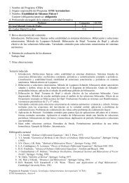
Figure 2.1: The characteristic densities <strong>and</strong> temperatures of different plasmas in nature <strong>and</strong><br />
produced in the labora<strong>to</strong>ry.<br />
16
Curso 2013-2014 <strong>An</strong> introduction <strong>to</strong> <strong>Plasma</strong> <strong>Physics</strong>, ...<br />
Since only Coulomb collisions between charged particles are relevant in fully ionized plasmas,<br />
the collisional processes with neutral a<strong>to</strong>ms introduce additional features.<br />
• Partially ionized plasmas are said collisional when the mean free path λ ≪ L for the<br />
relevant collisional processes are much smaller than the dimensions L of the medium.<br />
• The elastic <strong>and</strong> inelastic collisions between neutrals <strong>and</strong> charged particles in collisional<br />
plasmas give rise <strong>to</strong> a large number of physical processes as ionization, light emission,<br />
...etc.<br />
The plasmas can be roughly characterized by <strong>its</strong> kinetic temperature k B T <strong>and</strong> charged<br />
particle density density n. In Fig. (2.1) are classified a number of those found in nature <strong>and</strong><br />
also produced in the labora<strong>to</strong>ry. As we can see, the possible values for the particle densities in<br />
this figure covers twenty orders of magnitude (from 1 up <strong>to</strong> 10 25 charges by cubic centimeter).<br />
The corresponding temperature range is extended along seven orders of magnitude (from 10 −2<br />
up <strong>to</strong> 10 5 eV ).<br />
In order <strong>to</strong> grasp the huge extent of these scales it would be enough <strong>to</strong> introduce in the<br />
diagram of Fig. (2.1) the point corresponding <strong>to</strong> the water at room temperature n ≃ 2.1×10 22<br />
cm −3 , <strong>and</strong> for the ordinary air; the Loschmidt number n ≃ 2.7×10 19 cm −3 at STP conditions.<br />
The particle densities of air <strong>and</strong> liquid water only differ by a fac<strong>to</strong>r 10 3 . Between the ordinary<br />
water <strong>and</strong> the density of a white dwarf star this fac<strong>to</strong>r raises up <strong>to</strong> 10 15 , much shorter than<br />
the plasma density range of Fig. (2.1).<br />
2.2 <strong>Plasma</strong>s in astrophysics<br />
The cold k B T ∼ = 10 −2 − 10−1 eV interestellar plasma has a very low density of 10 −5 cm −3<br />
<strong>and</strong> does not appear in Fig. (2.1). This concentration as low as 0.1 charged particle by cubic<br />
meter leads Debye lengths in the order of 8 meters, that are used <strong>to</strong> scale the plasma equations.<br />
Thus, because of the huge distances involved the equations of magne<strong>to</strong>hidrodynamics could<br />
still be used <strong>to</strong> describe the plasma transport over galactic distances.<br />
Figure 2.2: The Sun chromosphere observed during an eclipse<br />
17
Escuela de Ingeniería Aeronáutica y del Espacio<br />
Universidad Politécnica de Madrid<br />
The plasma inside the Sun core where thermonuclear reactions take place has an estimated<br />
temperature about k B T ∼ = 10 5 eV <strong>and</strong> the densities are n ∼ 10 25 . At the solar corona the<br />
temperature decreases down <strong>to</strong> k B T ∼ = 10 − 10 2 eV <strong>and</strong> the density n ∼ 10 5 decreases about<br />
15 orders of magnitude over the surface of the Sun.<br />
The stellar atmospheres are constituted by a gases hot enough <strong>to</strong> be fully ionized <strong>and</strong> the<br />
plasma at the Sun chromosphere could be observed during solar eclipses as in Fig. (2.2). This<br />
plasma is later accelerated by different physical mechanisms <strong>to</strong> form the solar flares <strong>and</strong> the<br />
solar wind that reach the Earth ionosphere following the interplanetary magnetic field lines<br />
[3].<br />
The solar wind is constituted by an stream of charged <strong>and</strong> energetic particles coming from<br />
the the sun. The typical solar wind parameter are n = 3 − 20 cm −3 , k B T i < 50 eV <strong>and</strong><br />
k B T e ≤ 100 eV. The drift velocities of these charged particles close <strong>to</strong> the Earth are about<br />
300-800 Km s −1 . This flow of charged particles reaches the Earth orbit <strong>and</strong> interacts with the<br />
geomagnetic field forming a complex structure denominated magne<strong>to</strong>sphere that protects the<br />
Earth surface from these high energy particle jets. The average properties of the interplanetary<br />
plasma in our solar system solar corona <strong>and</strong> solar wind are also in Fig. (2.1) [3].<br />
2.3 Geophysical plasmas<br />
V i<br />
V e<br />
Ions<br />
B<br />
Electrons<br />
Magnetic field<br />
2R T<br />
Earth<br />
The interplanetary plasma <strong>and</strong> the solar wind interact<br />
with the geomagnetic field <strong>to</strong> for a complex structure. The<br />
geomagnetic field is a centered magnetic dipole ∼ 1/r 3<br />
up <strong>to</strong> distances about two Earth radii (R T = 6.371 Km)<br />
inclined 11 o with respect <strong>to</strong> the planet axis. For distances<br />
over 2 R T interacts with the solar wind <strong>and</strong> gives raise <strong>to</strong><br />
a complex structure denominated magne<strong>to</strong>sphere [3, 5]<br />
The basic physical mechanism is outlined in Fig. (2.3).<br />
Figure 2.3: The deviation of The Earth magnetic field decreases with the distance in the<br />
charged particles by the geomagnetic<br />
field.<br />
comes from the sun. The Lorentz force resulting from the<br />
direction <strong>to</strong>wards the dayside where a stream of particles<br />
perpendicular geomagnetic field deviates the flux charged particles around the Earth. The<br />
weak local magnetic field is in turn affected by this current of charged particles resulting<br />
a complex structure of magnetic field <strong>and</strong> electric currents around the Earth. Within the<br />
magne<strong>to</strong>sphere are located the Van Allen belts around the Earth that are constituted by<br />
energetic particles trapped by the geomagnetic field [3, 5]<br />
At the North <strong>and</strong> south poles, the Earth magnetic field is connected with the Sun magnetic<br />
field lines. The particles moving with parallel velocity <strong>to</strong> the field lines do not experience a<br />
deflecting force <strong>and</strong> precipitate <strong>to</strong>wards the Earth surface. The stream of charged particles<br />
is aligned with the local geomagnetic field <strong>and</strong> this is the origin of polar auroras which are<br />
strongly influenced by the solar activity. The existence of magne<strong>to</strong>spheres around the planets<br />
is a common feature in the solar system that prevents the energetic particles from reach most<br />
of the surface of planets [3, 6].<br />
All the planets in the solar system have a ionosphere connecting the high altitude atmosphere<br />
with the outer space. They have different characteristic in accordance <strong>to</strong> the particular<br />
18
Curso 2013-2014 <strong>An</strong> introduction <strong>to</strong> <strong>Plasma</strong> <strong>Physics</strong>, ...<br />
Altitude (Km)<br />
1000<br />
500<br />
300<br />
200<br />
100<br />
−<br />
e<br />
+ O + He<br />
He<br />
O<br />
H + N +<br />
N 2<br />
NO + O 2<br />
O +<br />
N + 2<br />
Ar<br />
2<br />
10 3 10 4 10 5 10 6 10 7 10 8<br />
Density ( part. / cm 3 )<br />
Figure 2.4: The altitude dependent chemical composition of the Earth ionosphere from Ref. [16].<br />
properties of the planetary magnetic field <strong>and</strong> the chemical composition of <strong>its</strong> atmosphere. The<br />
Earth’s ionosphere is a weakly ionized plasma present between 50 <strong>and</strong> 1000 Km of altitude<br />
below the magne<strong>to</strong>sphere ver the neutral atmosphere. The altitude dependent particle density<br />
relies on the sun activity <strong>and</strong> also on the night/day cycle. The orbiting spacecrafts move<br />
immersed in<strong>to</strong> this cold (k B T ≤ 0.1 eV <strong>and</strong> tenuous plasma with densities of n = 10 3 − 10 7<br />
cm −3 <strong>and</strong> a altitude dependent chemical composition as shown in Fig. (2.4) [6, 7, 16].<br />
In Table (2.1) are the main properties of ionospheric plasma for different altitudes. Here<br />
n e,i are respectively the electron <strong>and</strong> ion densities, λ D the Debye length, <strong>and</strong> the average mass<br />
of the ion is ¯m i . The temperatures are respectively T e,i <strong>and</strong> the collisional mean free paths<br />
λ e,i . The typical orbital speed is V o , the local gas pressure P a <strong>and</strong> T a the gas temperature [16]<br />
2.4 Labora<strong>to</strong>ry plasmas<br />
The plasmas produced in the labora<strong>to</strong>ry or for technological applications are also appear in the<br />
scheme of Fig. (2.1) covering from cold discharge plasmas up <strong>to</strong> the experiments in controlled<br />
fusion.<br />
The electric discharges in gases are the most traditional field of plasma physics investigated<br />
by I. Langmuir, Tonks <strong>and</strong> their co-workers since 1920. In fact, the nobel laureate<br />
Irvin Langmuir coined the term plasma in relation <strong>to</strong> the peculiar state of a partially ionized<br />
gas. Their original objective was <strong>to</strong> develop for General Electric Co. electric valves that could<br />
withst<strong>and</strong> large electric currents. However, when these valves were electrically connected<br />
low pressure glow discharges triggered inside. The low pressure inert gases become partially<br />
ionized, weakly ionized plasmas.<br />
19
Escuela de Ingeniería Aeronáutica y del Espacio<br />
Universidad Politécnica de Madrid<br />
Figure 2.5: A labora<strong>to</strong>ry experiment with an argon electric glow discharge (left) <strong>and</strong> an stable<br />
structure of different plasmas separated by double layers (right).<br />
Two examples of a low pressure argon discharge plasmas are in Fig. (2.5). The typical low<br />
pressure discharges are weakly ionized plasmas with densities between 10 6 - 10 14 cm −3 <strong>and</strong><br />
temperatures of k B T ∼ = 0.1 − 10 eV in the scheme of Fig. (2.1). In our everyday life these<br />
electric discharges are widely used in a large number of practical applications, as in metal arc<br />
welding, fluorescent lamps, ...etc.<br />
The relatively cold plasmas (k B T e = 0.05-0.5 eV) of high pressure arc discharges are employed<br />
in metal welding <strong>and</strong> are dense quite dense; up <strong>to</strong> 10 20 . On the opposite lim<strong>its</strong> are<br />
flames which in most cases cannot be strictly considered as a plasma because of their low<br />
ionization degree.<br />
The physics of the discharge plasmas <strong>and</strong> <strong>its</strong> applications constitutes a branch of <strong>Plasma</strong><br />
<strong>Physics</strong> <strong>and</strong> Refs. [10] <strong>and</strong> [13] are two comprehensive books on this subject.<br />
The plasma thrusters are employed for space propulsion <strong>and</strong> they impart momentum <strong>to</strong><br />
an spacecraft by means an accelerated plasma stream where the ions are accelerated along a<br />
fixed direction. Contrary <strong>to</strong> classical chemical thrusters, may be continuously working <strong>and</strong><br />
the specific impulse of these devices is quite better than chemical thrusters. More than 700<br />
models have been flown in particular for deep space exploration <strong>and</strong> orbit station keeping.<br />
The plasmas of these devices are produced by low pressure electric discharges with densities<br />
up <strong>to</strong> 10 14 <strong>and</strong> temperatures in the range 1-2 eV. The basic <strong>Plasma</strong> <strong>Physics</strong> involved in space<br />
propulsion <strong>and</strong> new developments are discussed in Refs. [14, 15].<br />
The themonuclear controlled fusion is the more promising application of plasma physics<br />
since 1952. The controlled thermonuclear reaction of deuterium <strong>and</strong>/or tritium a<strong>to</strong>ms <strong>and</strong><br />
is intended in order <strong>to</strong> produce waste amounts of energy. The reaction cross sections are<br />
appreciable for energies of reacting particles over 5 KeV. This would require <strong>to</strong> produce an<br />
stable plasma with temperatures in the range of 10 KeV. The plasma heating <strong>and</strong> confinement<br />
of such hot plasma still remains a unsolved problem <strong>and</strong> active field of research. We can see<br />
in Fig. (2.1) the plasma densities reached <strong>to</strong>day in these experiments are around 10 10 − 10 13<br />
cm −3 with the temperatures k B T e<br />
∼ = 10 2 − 10 3 eV.<br />
20<br />
The design <strong>and</strong> operation of the future plasma fusion reac<strong>to</strong>r is a scientific <strong>and</strong> technological
Curso 2013-2014 <strong>An</strong> introduction <strong>to</strong> <strong>Plasma</strong> <strong>Physics</strong>, ...<br />
Altitude (Km) 150 200 400 800 1200<br />
V o m/s 7.83 × 10 3 7.80 × 10 3 7.68 × 10 3 7.47 × 10 3 7.26 × 10 3<br />
N i,e cm −3 3.0 × 10 5 4.0 × 10 5 1.0 × 10 6 1.0 × 10 5 1.0 × 10 4<br />
k B T i K 700 1100 1600 2200 2600<br />
k B T e K 1000 2000 2800 3000 3000<br />
¯m i uma 28 24 20 14 10<br />
λ D cm 0.40 0.49 0.37 1.20 3.78<br />
λ e,i cm 5.0 × 10 5 1.0 × 10 5 1.0 × 10 5 1.0 × 10 6 1.0 × 10 7<br />
P a Torr 3.75 × 10 3 7.5 × 10 −10 1.5 × 10 −11 - -<br />
T a K 635 859 993 - -<br />
Table 2.1: The characteristics of ionospheric plasmas for different altitudes from Ref. [16]. The<br />
ion k B T i <strong>and</strong> electron k B T e temperatures are in Kelvin degrees, the average ion mass ¯m i is in<br />
a<strong>to</strong>mic mass un<strong>its</strong> <strong>and</strong> the local pressure in Torrs.<br />
challenge that requires intense international collaboration. Such a reac<strong>to</strong>r must work with<br />
plasmas where n = 10 13 − 10 16 cm −3 <strong>and</strong> k B T ∼ = 0.5-1.0 ×10 4 eV.<br />
21
3<br />
Bibliography, texbooks <strong>and</strong> references<br />
There are excellent textbooks on the <strong>Physics</strong> of <strong>Plasma</strong>s <strong>and</strong> these notes are not intended <strong>to</strong><br />
replace them. They serve as a support for the lectures <strong>and</strong> therefore, it seems advisable <strong>to</strong><br />
provide a complementary bibliography for the reader.<br />
3.1 Textbooks<br />
The following books are general texts of <strong>Plasma</strong> <strong>Physics</strong>. The first one is very popular at<br />
elementary level while the others contain chapters with more advanced <strong>to</strong>pics.<br />
• <strong>Introduction</strong> <strong>to</strong> plasma physics <strong>and</strong> controlled fusion. Vol 1: <strong>Plasma</strong> physics. 2nd ed. F.F.<br />
Chen. Plenum Press New York, USA (1984).<br />
• <strong>Introduction</strong> <strong>to</strong> plasma physics. R.J. Golds<strong>to</strong>n <strong>and</strong> P.H. Rutherford. Institute of <strong>Physics</strong><br />
Bris<strong>to</strong>l, UK (1995).<br />
• Physique de <strong>Plasma</strong>s. Jean-Marcel Rax. Dundod, Paris, France (2007).<br />
The following references are introduc<strong>to</strong>ry books <strong>to</strong> <strong>Plasma</strong> <strong>Physics</strong> with an special emphasis<br />
on astrophysical <strong>and</strong> space problems. The first is a comprehensive collection of articles covering<br />
many fields of interest <strong>and</strong> the second is a textbook on the <strong>Physics</strong> of <strong>Space</strong> <strong>Plasma</strong>s. Finally,<br />
the last one is of elementary level <strong>and</strong> includes sections with applications of fluid dynamics in<br />
astrophysics <strong>and</strong> <strong>its</strong> connections with plasma physics.<br />
• <strong>Introduction</strong> <strong>to</strong> <strong>Space</strong> <strong>Physics</strong>, edited by M.G. Kivelson <strong>and</strong> C.T. Russel.<br />
University Press, New York, (1995).<br />
Cambridge<br />
• <strong>Physics</strong> of <strong>Space</strong> <strong>Plasma</strong>s, an <strong>Introduction</strong>, GK Parks. Addison Wesley, Redwood City<br />
CA. USA, (1991).<br />
• <strong>Physics</strong> of Fluids <strong>and</strong> <strong>Plasma</strong>s. <strong>An</strong> <strong>Introduction</strong> for Astrophysicists. A. Rai Choudhuri.<br />
Cambridge University Press, Cambridge U.K. (1998).<br />
22
Curso 2013-2014 <strong>An</strong> introduction <strong>to</strong> <strong>Plasma</strong> <strong>Physics</strong>, ...<br />
3.2 Bibliography on space plasmas<br />
These references cover two particular <strong>to</strong>pics of interest in this course. The first is a through<br />
reference regarding the structure <strong>and</strong> properties of the Earth ionosphere. The orbiting spacecrafts<br />
<strong>and</strong> satellites move in<strong>to</strong> <strong>and</strong> also interact with this particular medium, these issues are<br />
discussed in the two additional references.<br />
• The Earth’s Ionosphere: <strong>Plasma</strong> <strong>Physics</strong> <strong>and</strong> Electrodynamics. M.C. Kelley. International<br />
Geophysical Series, Academic Press, San Diego CA, USA (1989).<br />
• A review of plasma Interactions with spacecraft in low Earth orbit. D. Hastings, J Geophys.<br />
Res. 79, (A13), 1871-1884, (1986).<br />
• <strong>Space</strong>craft environment interactions. S.D. Hastings. Cambridge University Press, Cambridge,<br />
UK (2004).<br />
3.3 References on gas discharge physics<br />
The following references on the physics of electric discharges are indispensable <strong>to</strong> calculate<br />
numeric estimates of transport coefficients, ionization rates, ... etc.<br />
• Basic data of plasma physics: The fundamental data on electrical discharge in gases. S.C.<br />
Brown. American Vacuum Society Classics American Institute of <strong>Physics</strong>, New York,<br />
USA (1994).<br />
• Gas discharge physics. Y.P. Raizer. Springer-Verlag, Berlin, Germany (1991).<br />
3.4 Additional material<br />
One can be found easily in servers across the internet lots of information regarding <strong>to</strong>pics<br />
covered in this course. Some of them also include free useful computer codes codes. This is<br />
not an exhaustive list but provides some reference web pages.<br />
• On the <strong>Physics</strong> of <strong>Plasma</strong>s:<br />
http://plasma-gate.weizmann.ac.il/direc<strong>to</strong>ries/plasma-on-the-internet/<br />
This web page contains links <strong>to</strong> practically all large groups of <strong>Plasma</strong> <strong>Physics</strong> around<br />
the world. It covers software, references, conferences, ...etc <strong>and</strong> remains continuously<br />
updated.<br />
• <strong>Space</strong> <strong>Physics</strong> Groups at NASA:<br />
http://xd12srv1.nsstc.nasa.gov/ssl/PAD/sppb/<br />
NASA has a wide range of activities in physics from space <strong>and</strong> a full division dedicated<br />
<strong>to</strong> <strong>Plasma</strong> <strong>Physics</strong> issues.<br />
23
Escuela de Ingeniería Aeronáutica y del Espacio<br />
Universidad Politécnica de Madrid<br />
• Naval Research Labora<strong>to</strong>ry:<br />
http://wwwppd.nrl.navy.mil<br />
The naval research labora<strong>to</strong>ry in the U.S. has a division of plasma physics which publishes<br />
a free <strong>and</strong> well-known NRL plasma physics formulary of commonly used formulas.<br />
• <strong>Plasma</strong> Simulation Group. Berkeley University:<br />
http://ptsg.eecs.berkeley.edu<br />
This group dedicated <strong>to</strong> the development of PIC codes <strong>to</strong> simulate plasmas <strong>and</strong> gaseous<br />
discharges. The codes These codes have a good graphical interface are open <strong>and</strong> can be<br />
downloaded from this server for free.<br />
24
4<br />
The elementary processes <strong>and</strong> the plasma equilibrium<br />
In ordinary fluids the energy <strong>and</strong> momentum is transported by the short range molecular<br />
collisions of the neutral particles. Their properties determine the transport coefficients of the<br />
neutral gas, as <strong>its</strong> viscosity or thermal conductivity. These a<strong>to</strong>mic <strong>and</strong> molecular encounters<br />
also are the relaxation mechanism that brings the system from a perturbed state back in<strong>to</strong> a<br />
new equilibrium.<br />
Most plasmas (see Fig. 2.1) of interest in space are weakly coupled, the average kinetic<br />
energy of particles dominates <strong>and</strong> is much larger than their electrostatic energies. These<br />
plasmas are constituted by electrons, a<strong>to</strong>ms, molecules <strong>and</strong> eventually charged dust grains,<br />
in a dynamic equilibrium where a large number of collisional processes between the plasma<br />
particles take place. As for ordinary fluids, the collisions at a<strong>to</strong>mic <strong>and</strong> molecular level also<br />
determine both, the transport properties <strong>and</strong> the relaxation of perturbations <strong>to</strong>wards the<br />
equilibrium state.<br />
The a<strong>to</strong>mic <strong>and</strong> molecular encounters determine the response of fluids <strong>and</strong> plasmas <strong>to</strong><br />
external perturbations. They also couple the motions of the different particle species that<br />
contribute <strong>to</strong> the transport properties. Additionally, the long range Coulomb forces in plasmas<br />
are involved in collisions between charged <strong>and</strong> neutral species.<br />
The physical <strong>and</strong> chemical properties of plasmas in nature are determined by the characteristics<br />
of the elementary processes at a<strong>to</strong>mic <strong>and</strong> molecular level, <strong>and</strong> the number of possible<br />
collisional processes is huge. In Tables (4.3) <strong>and</strong> (4.1) are shown the more relevant involving<br />
the ions, electrons <strong>and</strong> neutral a<strong>to</strong>ms or molecules. The chemical nature of the parent<br />
neutral gas (or gas mixture) influences the plasma properties. While most ions are produced<br />
by electron impact in noble gases as Argon the formation of negative ions is important in<br />
electronegative gases as is the molecular oxygen O 2 .<br />
The degree of ionization in the plasma also determines the relevant molecular processes. In<br />
weakly ionized plasmas, the concentration of charged particles n e <strong>and</strong> n i are much lower than<br />
the neutral a<strong>to</strong>m background density n a ≫ n e , n i ; the ratio n e /n a could be as low as 1/10 5 .<br />
Therefore, the collisions between charged particles <strong>and</strong> neutrals dominate. On the contrary,<br />
in fully ionized plasmas the long range Coulomb collisions between charged particles are the<br />
relevant collisional processes.<br />
Not all possible of a<strong>to</strong>mic collisions are equal likely <strong>and</strong> the relevance of a particular<br />
25
Escuela de Ingeniería Aeronáutica y del Espacio<br />
Universidad Politécnica de Madrid<br />
molecular process introduces additional length <strong>and</strong> times scales characterized by <strong>its</strong> mean free<br />
path <strong>and</strong> collision frequency. In this section are introduced some simple concepts from kinetic<br />
theory in order <strong>to</strong> relate the properties of a<strong>to</strong>mic <strong>and</strong> molecular collisions with the transport<br />
properties of low density plasmas. In the following we will restrict ourselves <strong>to</strong> binary collisions<br />
that involve two particles. These are dominant in weakly coupled plasmas while those with<br />
more than two particles are important in denser strongly coupled plasmas. This connection<br />
between the transport properties <strong>and</strong> the properties of molecular <strong>and</strong> <strong>and</strong> a<strong>to</strong>mic collisions<br />
is throughly discussed in the classical Refs. [17] <strong>and</strong> [18] <strong>and</strong> a modern approach is found in<br />
Ref. [19].<br />
4.1 The collision cross section<br />
A<br />
A<br />
Γ A<br />
= n A<br />
V A<br />
A<br />
A<br />
B<br />
B<br />
B<br />
B<br />
B<br />
A<br />
A<br />
C<br />
A<br />
The classical concept of collision cross section could<br />
be traced back <strong>to</strong> the early a<strong>to</strong>mic models of Thomson<br />
<strong>and</strong> Rutherford <strong>and</strong> considers the typical velocity<br />
of particles v large enough so that their quantum<br />
wavelengths λ = h/m v are negligible. In this classical<br />
picture the particles are represented by spherically<br />
symmetric centers of force <strong>and</strong> the quantum effects as<br />
well as <strong>its</strong> internal structure are neglected.<br />
S<br />
The basic concept may be introduced using the<br />
D<br />
scheme of Fig. (4.1). The flux Γ A = n A V A of monoenergetic<br />
incident particles pass through the surface S<br />
Figure 4.1: The one dimensional <strong>and</strong> collide with the B target particles. The particles<br />
stream of particles A across the surface A <strong>and</strong> B only react or are scattered when reaching a<br />
S with particles B.<br />
minimum distance R o or -equivalently- when lie within<br />
the equivalent surface σ o = πRo. 2 The number of such collision events Q AB produced by a<br />
single molecule B by time unit is,<br />
dQ AB<br />
dt<br />
= ˙Q AB = σ o × Γ A = σ o × (n a V A ) (4.1)<br />
representing the number of A particles that cross σ o by time unit. Thus, the <strong>to</strong>tal cross section<br />
σ o may be defined as the ratio,<br />
σ o = ˙Q AB<br />
Γ A<br />
= ˙Q AB<br />
n a V A<br />
(4.2)<br />
Next, the number q AB of collisions by volume <strong>and</strong> time un<strong>its</strong> is obtained from by multiplying<br />
Eq. (4.1) by the number density n B of particles,<br />
d q AB<br />
dt<br />
= n B ˙Q AB = σ o n b n a V A<br />
When the particles A are lost by the reaction A + B → C + D the rate ṅ A = − ˙q AB <strong>and</strong>,<br />
dn A<br />
dt<br />
= −σ o n A n B V A < 0 while for the C <strong>and</strong> D particles, ṅ C = n˙<br />
D = −ṅ A > 0<br />
26
Curso 2013-2014 <strong>An</strong> introduction <strong>to</strong> <strong>Plasma</strong> <strong>Physics</strong>, ...<br />
Therefore, we obtain a differential equation for n A that can be integrated in time,<br />
m p<br />
V p<br />
> θ<br />
π<br />
2<br />
σ = π R 2<br />
dn A<br />
n A<br />
= −(σ o n B V A ) dt which gives, n A (t) = n Ao e −ν t > 0<br />
where,<br />
ν = σ o n B V A<br />
Figure 4.2: Dispersed particles<br />
under large θ > π/2 <strong>and</strong> small<br />
θ < π/2 scattering angles.<br />
θ<br />
is the collision frequency. This magnitude represents the<br />
number of collisions of a given process by unit time. We<br />
may also introduce the length ν = V A /λ which gives collision<br />
mean free path,<br />
λ = 1/(σ o n B )<br />
representing the average length that the A particle travels between two successive collisions<br />
among the background of particles n B . Alternatively, using dx A = V A dt we also obtain,<br />
n A (x) = n Ao e −x/λ<br />
The equations for n A (x) <strong>and</strong> n A (t) respectively represents the attenuation in the number of<br />
particles with the beam depth x, <strong>and</strong> the decay in number with time. The collision cross<br />
section is involved in λ <strong>and</strong> ν <strong>and</strong> measures the characteristic time <strong>and</strong> length.<br />
The cross section σ o ∼ π R 2 o essentially measures the extent of the region with average<br />
radius R o where A <strong>and</strong> B interact. Note that in addition <strong>to</strong> the reactions the collisions also<br />
scatter the particles along large θ > π/2 or small θ < π/2 deflection angles as in Fig.(4.2). For<br />
two hard spheres with radius d A <strong>and</strong> d B the cross section is,<br />
σ o = πR 2 o with, R o = 1 2 (d A + d B )<br />
When a particles experience different kinds of collisions with cross sections σ <strong>to</strong>t = σ 1 +σ 2 +. . .<br />
the <strong>to</strong>tal collision frequency in above equation becomes ν <strong>to</strong>t = ν 1 + ν 2 + . . . .<br />
4.2 The <strong>to</strong>tal <strong>and</strong> differential cross sections.<br />
In the general, the cross section essentially depends on the relative velocity |v A − v B | = |g| = g<br />
of the colliding species <strong>and</strong> therefore the could no be considered as a constant value. Equivalently,<br />
on the kinetic energy E of the incoming particle in the frame where the target remains<br />
at rest (labora<strong>to</strong>ry frame). The incident particles also could be scattered along large or small<br />
scattering angles θ as in Fig. (4.2) or –because of the internal properties of colliding particles–<br />
along a privileged direction. This situation is depicted in the schemes of (4.3) <strong>and</strong> (4.4).<br />
As a first step we generalize the Eq. (4.1) by considering the number ∆ ˙Q AB of collision<br />
events by time unit between the A particles within the interval of velocity ∆v A as,<br />
∆ ˙Q AB<br />
∆v A<br />
∼ d ˙Q AB<br />
dv A<br />
27
Escuela de Ingeniería Aeronáutica y del Espacio<br />
Universidad Politécnica de Madrid<br />
Therefore, for a particular collisional process, the energy dependent <strong>to</strong>tal cross section is<br />
defined as,<br />
d ˙Q AB = n A σ T (|v A − v B |) |v A − v B | dv A (4.3)<br />
As in the Eq. (4.1) d ˙Q AB represents the number of collision events produced by a target<br />
molecule B for velocities of the incoming A particles between v A <strong>and</strong> v A + dv A . The <strong>to</strong>tal<br />
cross section may be also introduced by generalizing the Eq. (4.2) as the ratio,<br />
σ T (|v A − v B |) = (d ˙Q AB /dv A )<br />
Γ A<br />
= (d ˙Q AB /dv A )<br />
n A |v A − v B |<br />
The <strong>to</strong>tal cross section σ T (|v A − v B |) characterizes the energy dependent scattering of A<br />
particles irrespective of their dispersion angles.<br />
X<br />
Z<br />
B<br />
V A<br />
θ<br />
A<br />
A<br />
dθ<br />
dϕ<br />
Figure 4.3: The scheme of an<br />
a<strong>to</strong>mic collision.<br />
σ AB (|v A − v B |) = (d ˙Q AB /dv A dΩ)<br />
Y<br />
However, in accordance <strong>to</strong> their internal states, the incident<br />
particle A could be scattered over a preferred direction<br />
along the angle θ. The differential cross section<br />
σ AB (g, θ) accounts for this anisotropic scattering as indicated<br />
in Fig. (4.3).<br />
The incident particle moves along the Z axis <strong>and</strong> is<br />
scattered by the particle at rest located at the origin. The<br />
dispersion is independent of the angle φ 1 <strong>and</strong> the trajec<strong>to</strong>ry<br />
of the incoming particle <strong>and</strong> the Z axis are contained<br />
in the plane indicated in Fig. (4.3). Again, as in Eq. (4.1)<br />
the number collision events Q AB by time unit of A particles<br />
emerging within the solid angle dΩ = sin θ dθ dφ,<br />
d ˙Q AB (θ, g) = n A σ AB (g, θ) |v A − v B | sin θ dθ dφ (4.4)<br />
Again, the differential cross section could be also introduced<br />
using the Eq. (4.2) as the ratio,<br />
Γ A<br />
= (d ˙Q AB /dv A dΩ)<br />
n A |v A − v B |<br />
This represents the ration between the number of particles by time unit that appear over the<br />
solid angle dΩ after collide over the flux of incoming A particles.<br />
The integration over the angles dφ <strong>and</strong> dφ of Fig. (4.3) recovers the <strong>to</strong>tal cross section,<br />
therefore,<br />
dσ T (|v A − v B |) = σ AB (θ, |v A − v B |) dΩ<br />
σ T (|v A − v B |) =<br />
<strong>and</strong> we obtain the Eq. (4.3),<br />
∫ 2π ∫ 0<br />
0<br />
π<br />
σ AB (θ, |v A − v B |) sin θ dθ dφ<br />
1 The collisions may also depend on φ of Fig. (4.3) <strong>and</strong> the cross section would be as σ(E, θ, φ), but this<br />
situation is caused by the existence of internal states in the colliding molecules, however is unusual in a<strong>to</strong>mic<br />
28
Curso 2013-2014 <strong>An</strong> introduction <strong>to</strong> <strong>Plasma</strong> <strong>Physics</strong>, ...<br />
∫ π<br />
σ T (|v A − v B |) = 2π<br />
0<br />
σ AB (|v A − v B |, θ) sin θ dθ<br />
The values for the cross section are essentially determined in experiments where are analyzed<br />
the dispersion of an incident particle beam by a target material 2 . Additionally, the<br />
values for σ AB (θ, |v A − v B |) could be theoretically calculated by means of physical models<br />
that predicts the dispersion angles of particles observed in the experiments.<br />
In Figs. (4.6), (4.5) <strong>and</strong> (4.10) are some useful experimental values for the <strong>to</strong>tal cross<br />
section for the collisions of interest in labora<strong>to</strong>ry plasmas. These are discussed in [10] <strong>and</strong> [13]<br />
in the context of the physics of electric discharges. The differential cross sections for elastic<br />
collisions between low energy electrons <strong>and</strong> neutral Argon a<strong>to</strong>ms are in Fig. (4.7). Finally, the<br />
differential cross sections in relation with transport properties in plasmas are also discussed<br />
in Refs. [20, 21].<br />
4.3 Cross section <strong>and</strong> impact parameter<br />
The concepts of impact parameter <strong>and</strong> cross section are closely related <strong>and</strong> useful in a<strong>to</strong>m <strong>and</strong><br />
molecular collision experiments. For simplicity in the following we will consider the elastic<br />
dispersion of A particles by the B targets, but similar arguments apply <strong>to</strong> reactive collisions.<br />
In the classical experiments of particle scattering, the measurements essentially relate the<br />
so called impact parameter b(θ, E) <strong>and</strong> the energy E of the incident particle <strong>and</strong> <strong>its</strong> dispersion<br />
angle θ. This situation is depicted scheme of Fig. (4.4) in the frame where the target particle<br />
B remains at rest. We consider the symmetry around the angle φ <strong>and</strong> the incoming particle<br />
A moves again with relative speed g = v A − v B . After the collision event, the particle A is<br />
scattered along the angle θ with respect of <strong>its</strong> initial direction.<br />
The number of incoming particles by time unit entering in<strong>to</strong> the dashed annular surface<br />
δS = b db dφ of Fig. (4.4) is,<br />
( ) dnA<br />
= n A |g| δS = n A |g| (b db dφ)<br />
dt<br />
in<br />
where b is denominated the impact parameter. These particles are found after the encounter<br />
at the distance r from the dispersion center B within the spherical sec<strong>to</strong>r 2π r sin θ dθ.<br />
According <strong>to</strong> Eq. (4.4) the number of A particles emerging from the collision within the solid<br />
angle dΩ = sin θ dθ dφ may be expressed as,<br />
( ) dnA<br />
= n A |g| σ AB (θ, g) sin θ dθ dφ<br />
dt<br />
out<br />
Here, the differential cross section is σ AB (g, θ) <strong>and</strong> is adjusted <strong>to</strong> give,<br />
then,<br />
( ) dnA<br />
=<br />
dt<br />
in<br />
( ) dnp<br />
dt<br />
out<br />
<strong>and</strong> molecular encounters in gases.<br />
2 In the next section is discussed the useful Eq. (4.7) relating the cross section with the impact parameter.<br />
(4.5)<br />
29
Escuela de Ingeniería Aeronáutica y del Espacio<br />
Universidad Politécnica de Madrid<br />
(n AB |g|) b db dφ = (n AB |g|) σ AB (g, θ) sin θ dθ dφ (4.6)<br />
σ AB (θ, g) =<br />
b<br />
sin θ<br />
db<br />
∣dθ<br />
∣ (4.7)<br />
A b<br />
Therefore the cross section σ AB (θ, g) measures<br />
the variation of in the flux Γ = n A |g| of A particles<br />
g<br />
B ϕ Z<br />
in the collision along the scattering direction<br />
defined by the angle θ. The absolute value is introduced<br />
because b(E, θ) is usually a decreasing Figure 4.4: The A particle with impact<br />
function of θ, the particles with large impact parameter<br />
parameter b collides with relative velocity<br />
b are scattered along smaller angles θ. g = v A − v B <strong>and</strong> is scattered along the<br />
The theoretical models for molecular collisions direction θ.<br />
provide expressions for b(E, θ) that can be compared with the results of the experiments using<br />
Eq. (4.7). These concepts may be extended <strong>to</strong> reactive encounter. In this case, the particle<br />
found along the line defined by θ is the result of the reaction A + B <strong>and</strong> the Eqs. (4.5) <strong>and</strong><br />
(4.6) the number of molecular reactions.<br />
db<br />
dϕ<br />
<strong>and</strong> we finally obtain the relation between the dif-<br />
ferential cross section <strong>and</strong> the impact parameter,<br />
dΩ<br />
A<br />
θ<br />
4.4 The a<strong>to</strong>mic collisions in plasmas<br />
In plasmas electrons <strong>and</strong> charged particles are not bounded moving freely within the plasma<br />
bulk. The number of different collisional processes in the plasma is huge <strong>and</strong> scale with the<br />
number of particles involved. The more relevant processes for electrons are in Table (4.1) <strong>and</strong><br />
for ions <strong>and</strong> neutral a<strong>to</strong>ms in Table (4.3). All collisional processes could be roughly categorized<br />
[14] as;<br />
• Elastic: The <strong>to</strong>tal kinetic energy of colliding particles is conserved <strong>and</strong> also retain their<br />
charges <strong>and</strong> initial internal states.<br />
• Inelastic: A fraction of kinetic energy is transferred <strong>to</strong> alter the initial internal state of<br />
one (or both) colliding particles. Also <strong>to</strong> produce an additional particle, as in ionizing<br />
collisions.<br />
• Superelastic: A collision where potential energy is transformed in<strong>to</strong> kinetic energy so that<br />
the <strong>to</strong>tal kinetic energy of colliding object is greater after the collision than before 3 .<br />
• Radiative: When a fraction of the kinetic energy is radiated in any range of the electromagnetic<br />
spectrum.<br />
• Charge exchange: The electric charge state of colliding particles is interchanged. <strong>An</strong><br />
electric charge is transferred from one <strong>to</strong> other.<br />
3 This occurs for example in the electron ion recombination.<br />
30
Curso 2013-2014 <strong>An</strong> introduction <strong>to</strong> <strong>Plasma</strong> <strong>Physics</strong>, ...<br />
Figure 4.5: Experimental data of the elastic cross sections <strong>and</strong> collision probabilities between<br />
electrons <strong>and</strong> neutrals for different gases from Ref. [10].<br />
31
Escuela de Ingeniería Aeronáutica y del Espacio<br />
Universidad Politécnica de Madrid<br />
The detailed description of each a<strong>to</strong>mic collision depends of the energy of incident particles<br />
<strong>and</strong> their internal states. Our objective is not <strong>to</strong> review the elementary processes in detail but<br />
we will briefly examine their more relevant features for the low energy range of our interest.<br />
For more details on the theoretical models for cross sections end their experimental data the<br />
reader is referred <strong>to</strong> the literature on this subject. The Refs. [10], [11] <strong>and</strong> [12] discuss in<br />
detail the kinetic of charged particles <strong>and</strong> plasma chemistry.<br />
4.4.1 The electron collisions with neutrals<br />
Electrons are the more mobile particles in a plasma <strong>and</strong> when the gas is partially or weakly ionized,<br />
the collisions between electrons <strong>and</strong> neutral a<strong>to</strong>ms are dominant. Collisions with neutrals<br />
require the close approach of colliding p<strong>and</strong> therefore are of short range. In weakly ionized<br />
plasmas these cross sections are the major contribution <strong>to</strong> the plasma transport coefficients.<br />
4.4.1.1 The elastic collisions<br />
Cross Section (cm -2 )<br />
10 -15<br />
10 -16<br />
10 -17<br />
Elastic<br />
Ionization<br />
Excitation<br />
10 -1 10 0 10 1 10 2<br />
Energy (eV)<br />
Figure 4.6: The <strong>to</strong>tal cross sections of<br />
Argon for elastic <strong>and</strong> inelastic collisions<br />
between electron <strong>and</strong> neutral a<strong>to</strong>ms.<br />
In these collisions there is a negligible exchange (in<br />
the order of δ = (2m e /m a ) of kinetic energy between<br />
the electron <strong>and</strong> the neutral a<strong>to</strong>m. Then, the energy<br />
of colliding particles is practically conserved without<br />
changes in the internal states of the neutral a<strong>to</strong>m,<br />
e − + A → e − + A<br />
The <strong>to</strong>tal elastic cross sections for low electron energies<br />
in are Fig. (4.5) <strong>and</strong> exhibit strong variations<br />
<strong>and</strong> an important angular dependence for the electron<br />
scattering as shows the Fig. (4.7).<br />
The electron energy energy profiles (see Fig. 4.5)<br />
differ within an order of magnitude according <strong>to</strong> the<br />
chemical nature of molecular (N 2 , CO, O 2 ) <strong>and</strong> a<strong>to</strong>mic<br />
(Ar, Kr, Xe) gases. The values are about σ(E) ∼<br />
5.0 − 35.0 × 10 −16 cm −2 for noble gases.<br />
The elastic collisions take place for any energy of the incoming electron <strong>and</strong> the cross section<br />
decreases for large energies. The peak in the cross section for very low energies correspond <strong>to</strong><br />
a quantum mechanical effect denominated Ramssauer effect, which could be appreciated for<br />
Argon at low electron energies in Fig. (4.6).<br />
This growth of the cross section takes place when the characteristic size of the a<strong>to</strong>m<br />
(∼ 10 −8 cm) is in the order of the electron wavelength λ e = h/mv e . In this case the electron<br />
wave function interacts with those of electrons at the external shells of the a<strong>to</strong>m. On practical<br />
grounds the Ramssauer effect is negligible in most plasmas because the typical average electron<br />
energy leads a negligible number of low energy electrons.<br />
4.4.1.2 Inelastic collisions<br />
In the inelastic collisions a fraction of the initial electron kinetic energy is transferred <strong>and</strong><br />
produces changes in the internal state of the target particle. In this category are included<br />
32
Curso 2013-2014 <strong>An</strong> introduction <strong>to</strong> <strong>Plasma</strong> <strong>Physics</strong>, ...<br />
Electron collisions with a<strong>to</strong>ms <strong>and</strong> molecules<br />
Scheme Process Macroscopic effect<br />
1 e − + A + → e − + A + Elastic Coulomb collision between<br />
electron <strong>and</strong> ions<br />
2 e − + A → e − + A<br />
Elastic collision between electron<br />
<strong>and</strong> neutral a<strong>to</strong>ms<br />
3 e − + A → e − + A ∗ Excitation of neutrals by electron<br />
impact<br />
4 e − + AB → e − + AB ∗ ν Vibrational excitation<br />
5 e − + A → 2e − + A + Electron impact ionization<br />
6 e − + A ∗ → 2e − + A + Multistep ionization<br />
7 e − + AB → A + B − Dissociative attachement<br />
8 e − + A + B → AB − Three body attachment<br />
9 e − + AB → 2e − + A + B + Dissociative ionization<br />
10 e − + AB → e + A + B<br />
11 e − + A ∗ → e − + A<br />
Molecule dissociation by electron<br />
impact<br />
De-excitation of neutrals<br />
(quenching)<br />
12 2e − + A + → e − + A ∗ Three body recombination<br />
13 e − + A + → hν + A Radiative recombination<br />
14 e − + AB + → A + B ∗ Dissociative recombination<br />
15 e − + A − → 2e + A<br />
Detachment by electron impact<br />
Transport <strong>and</strong> energy transfer<br />
in highly ionized plasmas<br />
Electron transport <strong>and</strong> diffusion.<br />
Electron mobility<br />
Multiplication of metastable<br />
neutral a<strong>to</strong>ms<br />
Energy tranfer <strong>to</strong> vibrational<br />
levels of molecules<br />
Multiplication of ion <strong>and</strong> electrons<br />
from the ground state.<br />
Ionization of neutral a<strong>to</strong>ms<br />
from an excited state<br />
Production of negative ions in<br />
molecular gases<br />
Production of negative ions in<br />
electronegative gases<br />
Production a<strong>to</strong>mic ions in<br />
electronegative gases<br />
Production of neutral a<strong>to</strong>ms<br />
in molecular gases<br />
Destruction of metastable<br />
neutral a<strong>to</strong>ms<br />
Relevant in dense highly ionized<br />
plasmas<br />
Relevant in dense highly ionized<br />
plasmas<br />
Important in weakly ionized<br />
molecular plasmas<br />
Loss of negative ions in electronegative<br />
gases<br />
Table 4.1: The most relevant electron collisional processes in plasmas for energy exchange (1-4)<br />
production of particles (5-10) <strong>and</strong> losses (11-15). The neutral a<strong>to</strong>m is A, <strong>its</strong> metastable state<br />
A ∗ <strong>and</strong> A + represents the corresponding single charged ion. The molecules or dia<strong>to</strong>mic gases are<br />
indicated as AB.<br />
33
Escuela de Ingeniería Aeronáutica y del Espacio<br />
Universidad Politécnica de Madrid<br />
Low energy electron scattering from Argon<br />
σ( E, θ) × 10 16 cm 2 sr −1<br />
8.0<br />
4.0<br />
0.0<br />
0 30 60 90 120 150 180<br />
<strong>An</strong>gle<br />
5 eV<br />
10 eV<br />
20 eV<br />
30 eV<br />
50 eV<br />
Figure 4.7: Experimental data of the differential cross section for low energy electrons with Argon<br />
a<strong>to</strong>ms from Ref. [8].<br />
the collisions that transfer a fraction of the electron energy <strong>to</strong> the neutral a<strong>to</strong>m in which a<br />
bounded electron jumps in<strong>to</strong> excited state as,<br />
e − + A ∗ → e − + A +<br />
The corresponding cross section depends of the excited state of the neutral a<strong>to</strong>m. This<br />
latter is ionized in the electron impact ionization,<br />
e − + A → 2 e − + A +<br />
when the energy of the incident electron lies over the ionization energy E I of the neutral a<strong>to</strong>m.<br />
The ionization of a neutral produces an electron-ion pair <strong>and</strong> the newly released electron is<br />
called secondary electron.<br />
A plasma stable in time requires of an dynamic equilibrium between the charge production<br />
(ionization) <strong>and</strong> losses (recombination). The number of produced electron-ion pairs needs <strong>to</strong><br />
be equal <strong>to</strong> the number of those lost in order <strong>to</strong> obtain a plasma density constant in time.<br />
These inelastic collisions provide excited neutral a<strong>to</strong>ms <strong>and</strong> ions, <strong>and</strong> the electron impact<br />
ionization is usually the main charge production mechanism in the plasma. Both require of a<br />
threshold energy for the impacting electron.<br />
The elastic, excitation (only the more relevant transition is depicted) <strong>and</strong> ionization cross<br />
section or argon are compared 4 in Fig. (4.6). The qualitative dependence with the electron<br />
energy is similar in most gases.<br />
4 Note that the energies are represented in logarithmic scale.<br />
34
Curso 2013-2014 <strong>An</strong> introduction <strong>to</strong> <strong>Plasma</strong> <strong>Physics</strong>, ...<br />
10 0 10 1 10 2 10 3<br />
10 –1<br />
Helium<br />
Cross section σ(E) ( cm 2 )<br />
10 –2<br />
10 0<br />
10 –1<br />
10 –2<br />
He + × 10 –17 cm 2<br />
He ++ × 10 –19 cm 2<br />
10 1 10 2 10 3<br />
Neon<br />
Ne + × 10 –17 cm 2<br />
Ne ++ × 10 –17 cm 2<br />
10 1 10 1 10 2 10 3<br />
10 0 Argon<br />
Ar + × 10 –16 cm 2<br />
10 –1<br />
Ar ++ × 10 –17 cm 2<br />
Electron energy (eV)<br />
Figure 4.8: Experimental data from Ref. [9] for the electron impact ionization cross sections of<br />
different rare gases.<br />
35
Escuela de Ingeniería Aeronáutica y del Espacio<br />
Universidad Politécnica de Madrid<br />
The excitation <strong>and</strong> ionization require of a threshold value for the energy of the colliding<br />
electron <strong>and</strong> after a sharp growth decreases smoothly for high energies. When the transition of<br />
the bounded electron <strong>to</strong> the target neutral a<strong>to</strong>m is allowed according <strong>to</strong> the spectroscopy selection<br />
rules, the tail of σ(E) trend <strong>to</strong> decrease as σ(E) ∼ ln(E)/E while it falls as σ(E) ∼ 1/E<br />
or faster when is forbidden. In both inelastic collisions, the dispersed electrons are concentrated<br />
more around the forward direction than for the elastic collisions (see Fig. 4.7) <strong>and</strong> this<br />
tendency increases with the electron energy.<br />
ν I<br />
/ (n a<br />
C V Te<br />
)<br />
10 -1<br />
10 -2<br />
10 -3<br />
10 -4<br />
10 -5<br />
10 -6<br />
H E I<br />
= 13.6 eV<br />
He E I = 24.6 eV<br />
Ar E I<br />
= 15.8 eV<br />
10 -7<br />
0,5 1 1,5 2 2,5 3<br />
Electron temperature K B<br />
T e<br />
(eV)<br />
Figure 4.9: The growing of the ionization<br />
frequency with k B T e for a<strong>to</strong>mic H, He <strong>and</strong><br />
Ar using the Eq. (4.10).<br />
The inelastic collisions with a threshold energy<br />
produce changes in the electron energy distribution<br />
function. Since most excitation potential<br />
of gases are in the order of few eV, each collision<br />
event reduces the energy of the impacting<br />
electron by an amount E I . Therefore, the average<br />
energy of fast electrons in the tail of the energy<br />
distribution decreases, <strong>and</strong> these electrons return<br />
<strong>to</strong> the low energy group.<br />
The ionization rate could be calculated using<br />
the Eq. (4.3). The number ˙Q I of ionization<br />
events by target neutral a<strong>to</strong>m in the frame where<br />
they remain at rest is,<br />
d ˙Q I = n e σ I (v e ) |v e | dv e<br />
The number of incoming electrons with velocities between v e <strong>and</strong> v e + dv e is therefore,<br />
n e dv e = n eo f e (v e ) dv e<br />
<strong>and</strong> in the case of a isotropic electron distribution f e (v e ) = f e (|v e |) also,<br />
n e dv e = n eo g e (E) dE<br />
<strong>and</strong> g e (E) is the electron energy distribution function. Then,<br />
d ˙Q I = n eo σ I (v e ) v e f e (v e ) dv e = n eo σ I (v e ) v e g e (E) dE<br />
where σ I (E) is the cross section for electron impact ionization. The energy of the colliding<br />
electron needs <strong>to</strong> be over the ionization threshold E I = m e vI 2 /2 of the neutral a<strong>to</strong>m, so that<br />
σ I (E) = 0 for E < E I . Therefore,<br />
or equivalently,<br />
˙Q I = n eo<br />
∫ ∞<br />
v I<br />
σ I (v e ) v e f e (v e ) dv e (4.8)<br />
˙Q I = n eo<br />
∫ ∞<br />
E I<br />
σ I (E) v e g e (E) dE (4.9)<br />
36
Curso 2013-2014 <strong>An</strong> introduction <strong>to</strong> <strong>Plasma</strong> <strong>Physics</strong>, ...<br />
Gas He H 2 Ne N 2 O 2<br />
C 0.13 0.59 0.16 0.85 0.68<br />
Table 4.2: Coefficient C in the electron impact cross section for ionization (Eq. 4.10) for different<br />
gases from Ref. [10].<br />
Higher ionization levels of ions as double ionized ions (as A ++ , ...etc) have lower cross<br />
sections <strong>and</strong> require of higher energies for ionizing electrons. This fact is evidenced in the<br />
experimental data of Fig. (4.8) where the energy threshold for the double ionization of rare<br />
gases corresponds <strong>to</strong> higher energies of the impacting electron.<br />
As observed in Fig. (4.6) the ionization cross section grows fast σ I (E) grows fast for<br />
electron energies over E ≥ E I . Therefore, in Eq. (4.8) is usually approximated by a piecewise<br />
linear function,<br />
{<br />
σ I (E) =<br />
0 if E < E I<br />
C (E − E I ) if E ≥ E I<br />
(4.10)<br />
where C is an empirical value <strong>and</strong> in Table (4.2) are their values for different gases. For a<br />
Maxwellian electron energy distribution function (Eqs. 1.1 <strong>and</strong> 1.2) with temperature k B T e<br />
in Eqs. (4.8) <strong>and</strong> (4.9) we obtain,<br />
where A = n a C ¯v e <strong>and</strong> ¯v e is given by Eq.(1.3).<br />
ν I = A (1 + 2k B T e ) exp(−E I /k B T e ) (4.11)<br />
In Fig. (4.9) is represented the ratio ν I /A which only rely on the electron temperature. As<br />
it could be observed, the ionization frequency grows several orders of magnitude with the<br />
electron temperature. The increasing value of k B T e produce a wider Maxwellian distribution<br />
for electrons <strong>and</strong> the number of electrons in the tail for energies E > E I also increments. A<br />
higher number of electrons with energy enough <strong>to</strong> produce a ionization event increases the<br />
ionization rate in the plasma.<br />
The ionization from the ground state of the neutral a<strong>to</strong>m is not the only possibility. The<br />
ion could also be produced by two successive collisions, from an excited level of the of the<br />
neutral,<br />
A + e − → A ∗ + e −<br />
<strong>and</strong> then,<br />
A ∗ + e − → A + + e − .<br />
Finally, the electrons could be also los in certain gases by attachment.<br />
formed by capturing an electron as,<br />
N 2 + e − → N − 2<br />
This occurs for certain molecular gases in accordance <strong>to</strong> their electron affinity.<br />
A negative ion in<br />
37
Escuela de Ingeniería Aeronáutica y del Espacio<br />
Universidad Politécnica de Madrid<br />
4.4.2 Ion collisions with neutrals<br />
In plasma whit low ionization degrees the elastic collisions between ions <strong>and</strong> neutral a<strong>to</strong>ms<br />
are frequent. <strong>An</strong> important process is the collision between a neutral <strong>and</strong> an ion where an<br />
electron is interchanged, denominated charge exchange collision,<br />
A + + B → B + + A<br />
<strong>and</strong> these collisions are dominant in partially <strong>and</strong> weakly ionized plasmas.<br />
The charge exchange is resonant when both colliding a<strong>to</strong>ms have similar ionization energies<br />
<strong>and</strong> non resonant otherwise. As it can be deduced from the experimental data of Figs.<br />
(4.10) <strong>and</strong> (4.5) this reaction has a cross sections 5 comparable with those for elastic collisions<br />
between electrons <strong>and</strong> neutral a<strong>to</strong>ms <strong>and</strong> contributes <strong>to</strong> distribute the positive charges within<br />
the plasma. In weakly ionized plasma where the number of ions is low <strong>and</strong> the neutral a<strong>to</strong>m<br />
concentration high, these collisions represent <strong>and</strong> important mechanism for energy transfer<br />
between both species.<br />
The electrons are not the only particle producing the ionization of a neutral. There ex<strong>its</strong><br />
ion neutral collisions where charges are produced as in the dissociative ionization where two<br />
neutrals collide, one of them excited,<br />
A ∗ + B → A + + B + e − .<br />
Again, a large number of possible molecular <strong>and</strong> a<strong>to</strong>mic collisions are possible <strong>and</strong> the details<br />
are beyond the scope of these notes.<br />
4.4.3 Pho<strong>to</strong>processes<br />
In radiative collisions or pho<strong>to</strong>processes the pho<strong>to</strong>n is the second particle involved <strong>and</strong> the<br />
kinetic energy of a particle may be transformed in electromagnetic radiation. For example, in<br />
the pho<strong>to</strong>ionization process the ionizing particle is a quantum of light (pho<strong>to</strong>n) with energy<br />
E ν = h ν. When the energy E ν > E I is over the ionization potential of the neutral a<strong>to</strong>m,<br />
A + hν → A + + e − .<br />
The number of ionization events by time <strong>and</strong> volume is proportional <strong>to</strong> the concentration<br />
of neutral a<strong>to</strong>ms ν I = I(ν) n a , multiplied by a function I(ν) which rely in the light intensity<br />
(that is, <strong>to</strong> the number of available pho<strong>to</strong>ns) <strong>and</strong> the frequency ν of light.<br />
Additionally, the pho<strong>to</strong>excitation could increment the energy of an electron in the external<br />
shell of the neutral a<strong>to</strong>m which is eventually ionized later by an electron impact,<br />
A + hν → A ∗<br />
A ∗ + e − → A + + e −<br />
5 Some authors ambiguously use <strong>to</strong>tal cross section also for the sum of different <strong>to</strong>tal cross sections as in Fig.<br />
(4.10).<br />
38
Curso 2013-2014 <strong>An</strong> introduction <strong>to</strong> <strong>Plasma</strong> <strong>Physics</strong>, ...<br />
Ion <strong>and</strong> neutral a<strong>to</strong>m collisions<br />
Scheme Process Macroscopic effect<br />
1 A + A → A + A<br />
2 A + + A → A + + A<br />
3 A + B + → A + + B<br />
4 A + A ∗ → A ∗ + A<br />
Elastic collision between neutral<br />
a<strong>to</strong>ms<br />
Elastic collision between ions<br />
<strong>and</strong> neutral a<strong>to</strong>ms<br />
Resonant or nonresonant<br />
charge exchange<br />
Collision between metastable<br />
<strong>and</strong> neutral a<strong>to</strong>ms<br />
5 A ∗ + B → e − + A + B + Penning ionization<br />
6 A + B ∗ → e − + AB + Associative ionization<br />
7 A + B + + C → A + BC + Ion association<br />
8 A ∗ + A ∗ → e − + A + + A Cross Penning reaction<br />
9 AB − + AB + → AB + AB Ion-ion recombination<br />
Transport of neutrals <strong>and</strong> energy<br />
thermalization<br />
Transport of ions, diffusion<br />
<strong>and</strong> thermalization of energy<br />
Ion transport, diffusion <strong>and</strong><br />
thermalization of energy<br />
Diffusion of metastable a<strong>to</strong>ms<br />
Production ions in gas<br />
mixtures<br />
Production of molecular ions<br />
in dia<strong>to</strong>mic or gas mixtures<br />
Production of molecular ions<br />
in gas mixtures<br />
Production of ions from<br />
metastable a<strong>to</strong>ms<br />
Loss of negative ions in electronegative<br />
or dia<strong>to</strong>mic gases<br />
Table 4.3: Relevant collisional processes between ions <strong>and</strong> neutral a<strong>to</strong>ms in plasmas involving<br />
energy exchange (1-4) ion production (5-8) <strong>and</strong> losses. The neutral a<strong>to</strong>m is A, <strong>its</strong> metastable state<br />
A ∗ <strong>and</strong> A + represents the corresponding single charged ion. The molecules or dia<strong>to</strong>mic gases are<br />
indicated as AB<br />
39
Escuela de Ingeniería Aeronáutica y del Espacio<br />
Universidad Politécnica de Madrid<br />
40<br />
150<br />
Cross section σ(E) × 10 −16 (cm 2 )<br />
30<br />
20<br />
10<br />
0<br />
50<br />
40<br />
30<br />
20<br />
10<br />
80<br />
60<br />
40<br />
Helium<br />
Total<br />
Elastic<br />
Charge exchange<br />
Neon<br />
Argon<br />
100<br />
50<br />
150<br />
100<br />
50<br />
250<br />
200<br />
150<br />
100<br />
20<br />
0 5 10 15 20 25<br />
Energy (eV)<br />
0<br />
Collision Probability Pc (cm −1 Torr −1 )<br />
Figure 4.10: Experimental data from Ref. [10] for cross section <strong>and</strong> probabilities of elastic<br />
collisions between ions <strong>and</strong> neutral a<strong>to</strong>ms for different inert gases as a function of the ion energy.<br />
The data correspond <strong>to</strong> elastic collisions (diamonds), charge exchange (squares) <strong>and</strong> the sum of<br />
both (solid bullets).<br />
40
Curso 2013-2014 <strong>An</strong> introduction <strong>to</strong> <strong>Plasma</strong> <strong>Physics</strong>, ...<br />
The frequencies of light involved in pho<strong>to</strong>excitation are in the order of 1-5 eV, within<br />
the range of visible light ( E = 2.26 eV or λ = 550 nm ). The visible light emitted by<br />
plasmas comes mostly from these processes a<strong>to</strong>mic excitation <strong>and</strong> processes caused by the<br />
large number of free electrons with energies in the range 1-5 eV. However, the energies required<br />
<strong>to</strong> ionize the neutral a<strong>to</strong>ms from their ground state corresponds <strong>to</strong> the ultraviolet part of the<br />
electromagnetic spectrum.<br />
4.4.4 The collisions of charged particles<br />
The number of encounters between charged particles depend on the ionization degree,<br />
α = n i /(n i + n a )<br />
of the neutral gas. The plasmas may be roughly considered as fully ionized <strong>and</strong> the coulomb<br />
collisions dominant when the ionization degree is over few parts over one thous<strong>and</strong>, while can<br />
be neglected in weakly ionized plasmas. The long range electric force between two charged<br />
particles is more intense <strong>and</strong> is exerted at much longer distances that the average a<strong>to</strong>mic<br />
dimensions. The corresponding cross sections are therefore much larger than in collisions with<br />
neutral particles. Again, there are different possible collisions between charged particles <strong>and</strong><br />
we only discuss the more relevant.<br />
4.4.4.1 The electron <strong>and</strong> ion recombination<br />
The reverse process of ionization is the recombination of an electron e − <strong>and</strong> the ion A + <strong>to</strong><br />
produce a neutral a<strong>to</strong>m. There exists different possible a<strong>to</strong>mic <strong>and</strong> molecular processes that<br />
end with the production of a neutral a<strong>to</strong>m. However, the average number of ions lost by<br />
volume <strong>and</strong> time un<strong>its</strong> is proportional <strong>to</strong> the concentration of ions <strong>and</strong> electrons,<br />
( dn i<br />
dt ) rec = k R n e n i . (4.12)<br />
Here k R is the recombination rate, <strong>and</strong> a plasma stable in time <strong>and</strong> electrically neutral<br />
requires n i = n e = n. This leads <strong>to</strong> the following differential equation,<br />
<strong>and</strong> integrating we obtain,<br />
dn<br />
dt = −k R n 2<br />
1<br />
n = 1 n o<br />
+ k R t<br />
where n o is the ion (or electron) concentration at t = 0. The recombination coefficient k R<br />
could be experimentally determined by <strong>its</strong> linear relation of 1/n with time. The typical values<br />
found are k R ≃ 10 −7 cm 3 seg −1 .<br />
In addition <strong>to</strong> the electron impact ionization, the neutrals could be ionized <strong>and</strong> the ions<br />
recombined by different collisional processes. It must be emphasized that the corresponding<br />
41
Escuela de Ingeniería Aeronáutica y del Espacio<br />
Universidad Politécnica de Madrid<br />
reaction rate constants <strong>and</strong> the involved energies may differ by orders of magnitude. The<br />
relevance of each particular recombination process in the above average needs <strong>to</strong> be examined.<br />
The number of charged particles in a plasma in equilibrium is therefore related with the<br />
ionization frequency ν I (or equivalently with the reaction rate k I ) <strong>and</strong> the reaction rate k R .<br />
The equilibrium between charge production <strong>and</strong> recombination is determined by the quotient,<br />
n i<br />
n a<br />
= k I<br />
k R<br />
In labora<strong>to</strong>ry plasmas, the ions are lost mainly by recombination at the walls of the device,<br />
not in the plasma bulk. Because of the low ionization degrees, the typical recombination mean<br />
free path is larger than the physical dimensions of the plasma container. On the contrary, most<br />
of ions reach the plasma chamber walls without a recombining collision that would transform<br />
the ion in<strong>to</strong> a neutral a<strong>to</strong>m.<br />
4.4.4.2 The Coulomb collisions<br />
The long range Coulomb collisions of the form,<br />
A + + e − → A + + e − .<br />
transfer energy <strong>and</strong> momentum between the charged species. These collisions are dominant<br />
in fully ionized plasmas <strong>and</strong> in dense plasma may involved more than two particles.<br />
This is not the place for a detailed description of these collisions, however, it may be shown<br />
the using τ = λ ei /V th the average collision time between electrons <strong>and</strong> ions in MKSC un<strong>its</strong><br />
respectively are,<br />
<strong>and</strong><br />
τ e = 6√ 2 π 3/2 √<br />
ɛ o me Te<br />
3/2<br />
Λ e 4 n<br />
τ i = 12 √ π3/2 ɛ o mi T 3/2<br />
i<br />
Λ e 4 n<br />
(4.13)<br />
(4.14)<br />
Here, Λ = ln(d max /d min ) is the Coulomb logarithm proportional <strong>to</strong> the logarithm of the<br />
ratio the maximum <strong>and</strong> minimum impact parameters. The shortest approaching distance is<br />
d min <strong>and</strong> d min ≃ r c = e 2 /4πɛ o T determined by,<br />
m e,i u 2 e,i<br />
2<br />
−<br />
e2<br />
4πɛ o r c<br />
= 0<br />
Because the electric potential is shielded d max = λ d (the Debye length). The Coulomb logarithm<br />
is an smooth function of the density <strong>and</strong> plasma temperature.<br />
4.5 Numerical estimates<br />
The mean free paths, collision frequencies are estimated from the experimental data for cross<br />
sections. In addition, most of these quantities are somehow related with the neutral gas<br />
pressure, that we associate with the neutral a<strong>to</strong>m density n a through,<br />
42
Curso 2013-2014 <strong>An</strong> introduction <strong>to</strong> <strong>Plasma</strong> <strong>Physics</strong>, ...<br />
n a = 1<br />
k B<br />
P<br />
T = 7.24 × 10²² P T<br />
with the pressures in Torr 1 Pa = 133 Torr <strong>and</strong> neutral a<strong>to</strong>m densities in cm −3 we have,<br />
for the T a = 273 K we have<br />
n a [cm −3 18 P [Torr]<br />
] = 9.63 × 10<br />
T [K]<br />
n a [cm −3 ] = 3.53 × 10 16 P [Torr]<br />
The actual parameter measured in the experiments is the collision probability P c , which<br />
is defined as the average number of collisions experienced by a particle when traveling 1 cm of<br />
length at the temperature of o C <strong>and</strong> at the pressure of 1 mm Hg.<br />
The relation between P c <strong>and</strong> σ is simple. Being n b the density of target particles <strong>and</strong><br />
ν the collision frequency P c = ν ∆t (1 cm), <strong>and</strong> because ∆t(1 cm) = 1/v T where v T is the<br />
corresponding thermal velocity,<br />
P c = ν ∆t(1 cm) = (n b σ v T ) ×<br />
( ) 1 cm<br />
= n b σ<br />
v T<br />
For example, in collisions between neutrals <strong>and</strong> electrons (see Fig. 4.5) we have, P c = n a σ ea<br />
we have,<br />
<strong>and</strong> for the frequency,<br />
λ ea = 1<br />
n a σ ea<br />
= 1<br />
p o P c<br />
ν ea =<br />
v<br />
λ ea<br />
= p o P c v T e<br />
where p o =1 mm Hg, <strong>and</strong> for the <strong>to</strong>tal cross section we have,<br />
The cross sections are frequently expressed as,<br />
<strong>and</strong> results σ = 0.322 P c [Å 2 ].<br />
σ ea [cm −2 ] = 0.283 × 10 −16 P c<br />
σ = πa 2 o = 8.797 × 10 −17 cm −2 = 0.88 Å 2<br />
The experimental cross section for the elastic <strong>and</strong> inelastic collisions between electrons <strong>and</strong><br />
neutral a<strong>to</strong>ms for different gases as a function of the energy of the incident particle are in Figs.<br />
(4.5) <strong>and</strong> (4.6). Additionally, the cross sections for elastic <strong>and</strong> charge exchange collisions of<br />
ions with neutrals are in Fig. (4.10).<br />
43
Escuela de Ingeniería Aeronáutica y del Espacio<br />
Universidad Politécnica de Madrid<br />
4.6 The equilibrium states of a plasma<br />
As we have seen, not all the above reactions between the plasma species have equal probability.<br />
Their cross sections are different, the collision rates also rely on the degree of ionization, the<br />
concentration of ions, electrons, ...etc.<br />
Consequently, the plasma in thermodynamic equilibrium is a rather unusual situation in<br />
nature. Strictly speaking, it would require the balance of all collisional <strong>and</strong> radiative processes<br />
by the reverse reactions. So that the charge production <strong>and</strong> ionization rates must be equals,<br />
the emission <strong>and</strong> absortion of electromagnetic radiation by the plasma particles, ...etc. We<br />
conclude that,<br />
A plasma (or any other statistical population of particles) is in thermodynamic<br />
equilibrium when the rates of collisional <strong>and</strong> radiative processes are balanced by<br />
their reverse reactions.<br />
In such situation, the plasma is fully characterized by <strong>its</strong> thermodynamic magnitudes; the<br />
equilibrium pressure, volume <strong>and</strong> temperature. The energy distribution of each specie in the<br />
plasma is a Maxwell Boltzmann distribution with a common temperature for all species in the<br />
system. In this thermodynamic equilibrium state,<br />
• The physical properties properties of the plasma are uniform in space <strong>and</strong> constant in<br />
time.<br />
• The plasma is said optically thick. The balance of forward <strong>and</strong> backward reaction requires<br />
that the light produced by inelastic particle collisions is later absorbed <strong>and</strong> cannot leave<br />
the plasma region. In consequence, a plasma in thermodynamic equilibrium has a black<br />
body radiation spectrum.<br />
Obviously, these requisites are very restrictive <strong>and</strong> plasmas in thermodynamic equilibrium<br />
are seldom found in nature nor in labora<strong>to</strong>ry. In practice we always deal with plasmas far<br />
from thermodynamic equilibrium where the lack of balance of some elementary processes leads<br />
<strong>to</strong> a hierarchy of partial equilibrium states.<br />
The plasma is in local equilibrium when all collisional processes for charge production<br />
are balanced with those of particle recombination, but not the radiative<br />
processes.<br />
Under these conditions, the plasma in local equilibrium em<strong>its</strong> light, since it comes from radiative<br />
processes, as i.e. from electron impact excitation <strong>and</strong> deexcitation of bounded electrons<br />
of neutrals a<strong>to</strong>ms. This radiation leaves the plasma <strong>and</strong> therefore can be detected. However,<br />
the balance of all collisional processes between charged <strong>and</strong> neutral species implies that they<br />
are in equilibrium, <strong>and</strong> consequently, are again characterized by the Maxwell Boltzmann energy<br />
distribution with the same kinetic temperature.<br />
Finally, because of their the different cross sections in plasmas confined in small volumes<br />
only some collisional processes are balanced. This brings the next kind of plasma equilibrium.<br />
44
Curso 2013-2014 <strong>An</strong> introduction <strong>to</strong> <strong>Plasma</strong> <strong>Physics</strong>, ...<br />
The plasma is in partial equilibrium when only an small number of elementary<br />
processes are balanced.<br />
This is the more frequent situation in labora<strong>to</strong>ry plasmas because the charge production<br />
occurs within the plasma volume but the recombination of charged particles takes place at<br />
the walls of the plasma container or over the surface of the metallic electrodes.<br />
The reason is the electron impact ionization cross section, which is often much larger<br />
than the recombination cross section. Consequently, the ionization mean free path is shorter<br />
than for recombination. The charges are originated inside the plasma bulk but leave the<br />
experimentation volume without experience the corresponding recombining collision.<br />
4.6.1 Multithermal equilibrium<br />
A particular feature of plasmas is the possibility of<br />
the coexistence of charged particle populations with<br />
different average energies. This means a partial equilibrium<br />
where the electron k B T e <strong>and</strong> ion k B T i temperatures<br />
differ.<br />
The energy exchange between the different particle<br />
species is determined by the nature <strong>and</strong> frequency<br />
of collisions among them. Because of the disparity between<br />
the electron <strong>and</strong> ion masses the energy exchange<br />
is low in the elastic collisions between electrons <strong>and</strong><br />
neutral a<strong>to</strong>ms. The fraction of exchanged energy is<br />
proportional <strong>to</strong> δ = 2 m e /m i which typically lies between<br />
10 −4 <strong>and</strong> 10 −5 .<br />
The electron impact inelastic collisions produce<br />
transitions between energy levels of bounded electrons<br />
of a<strong>to</strong>ms <strong>and</strong> vibrational <strong>and</strong>/or rotational energy levels of molecules.<br />
Temperature (Kelvin)<br />
10 5<br />
10 4<br />
10 3<br />
K B<br />
T e<br />
K B<br />
T a<br />
10 2 10 −4 10 −3 10 −2 10 −1 1 10 1 10 2 10 3<br />
Gas Pressure (KPa)<br />
Figure 4.11: The neutral gas k B T a<br />
<strong>and</strong> electron k B T e temperatures as a<br />
function of the gas pressure.<br />
The typical energy<br />
transfer rate for these inelastic collisions is one or two orders of magnitude higher, between<br />
10 −3 <strong>and</strong> 10 −2 . On the contrary, for elastic <strong>and</strong> charge exchange collisions between ions <strong>and</strong><br />
neutral a<strong>to</strong>ms the energy exchange rate is much larger because colliding particles have similar<br />
masses. In other words, ions <strong>and</strong> neutrals share energy fast while electrons retain their kinetic<br />
energies during longer times.<br />
This effect of energy transfer between two plasma species is evidenced in Fig. (4.11) where<br />
are represented the electron k B T e <strong>and</strong> neutral gas k B T a temperatures as a function of the<br />
neutral gas pressure p a . The electrons acquire energy from the low electric field in the plasma<br />
<strong>and</strong> transfer a fraction of this energy <strong>to</strong> the neutral gas, essentially by elastic collisions.<br />
For low neutral pressures the collisions are scarce, the energy transfer between both species<br />
remains low <strong>and</strong> their respective temperatures are different. For higher gas pressures the<br />
collision frequency increases <strong>and</strong> both temperatures approach because the collisional energy<br />
transfer grows. In this partial equilibrium state of electrons ions <strong>and</strong> neutral a<strong>to</strong>ms the average<br />
electron kinetic energy per particle is different from those of ions <strong>and</strong> neutrals.<br />
Therefore the electron kinetic temperature k B T e ≫ k B T i differs from ion <strong>and</strong> neutral a<strong>to</strong>m<br />
temperatures k B T i ≃ k B T a . In the multithermal equilibrium state or two temperature plasma<br />
45
Escuela de Ingeniería Aeronáutica y del Espacio<br />
Universidad Politécnica de Madrid<br />
each charged particle specie is characterized by a different energy distribution function <strong>and</strong><br />
contrary <strong>to</strong> a plasma in local equilibrium. This partial equilibrium state of a plasma is often<br />
found in nature <strong>and</strong> in the labora<strong>to</strong>ry but obviously requires of an external source of energy<br />
<strong>to</strong> exist.<br />
4.6.2 The local equilibrium<br />
As we have seen, the Maxwell Boltzmann distribution corresponds <strong>to</strong> a plasma in thermodynamic<br />
equilibrium with parameters as temperatures <strong>and</strong> density constant in time <strong>and</strong> uniform<br />
in space. This fact excludes the possibility of transport of charged or neutral particles, momentum,<br />
energy, ...etc. Such situation has no practical interest because we usually deal with<br />
plasmas far from equilibrium. The determination of the nonequilibrium velocity (or energy)<br />
distribution function f α (v, r, t) for all plasma species (α = a, e, i) is a difficult task <strong>and</strong> one<br />
of the main objectives of the kinetic theory of plasmas.<br />
However, when certain conditions are met we may locally approximate this undetermined<br />
nonequilibrium energy distribution function by Eq. (1.1). That is, <strong>to</strong> consider the plasma<br />
species as locally Maxwellians by using,<br />
m α<br />
f α (v, r t) = n α (r, t) (<br />
2πk B T α (r, t) )3/2 exp<br />
(− m αv 2 )<br />
2k B T α (r, t)<br />
(4.15)<br />
where the density n α ( r, t) <strong>and</strong> temperature k B T α ( r, t) are non-uniform <strong>and</strong>/or time dependent.<br />
This approximation has the implicit assumption of the existence of fast energy relaxation<br />
processes in the plasma, or equivalently, of large collision frequencies. The collisions lead<br />
the energy fluctuations <strong>to</strong> relax fast <strong>to</strong> an local equilibrium state described by the Maxwell<br />
Boltzmann distribution. This local Maxwellian approximation is therefore valid when the<br />
spatial <strong>and</strong> time changes in the plasma properties are much lower that the characteristic time<br />
<strong>and</strong> length scales for collisions.<br />
Then, the essential requisite is that the plasma properties slowly vary in time <strong>and</strong> have<br />
smooth changes in space. The local Maxwellian distribution of the Eq. (4.15) may be unders<strong>to</strong>od<br />
as resulting from an small perturbation f 1 α(v, r, t) of Eq. (1.1) as,<br />
where |f 1 α| ≪ |f o α|.<br />
f α (v, r t) = f o α(v) + f 1 α(v, r, t)<br />
Then, the properties of this plasma obviously are neither constant in time nor homogeneous<br />
in space. The restrictive requisites for thermodynamic equilibrium condition are therefore<br />
weaken, <strong>and</strong> non equilibrium phenomena, as the particle transport are considered. Nevertheless,<br />
it should be stressed that the local Maxwellian plasma constitutes a useful approximation<br />
but is not the actual velocity distribution function of the plasma species.<br />
46
5<br />
The physical models for plasmas<br />
In Chapter 1.1 we introduced the plasmas as a mixture of interacting electrons, ions <strong>and</strong> neutral<br />
a<strong>to</strong>ms in thermodynamic equilibrium. In this situation, all particle species are described by<br />
a Maxwell Boltzmann energy distribution with a common temperature k B T e = k B T i = k B T a .<br />
The plasma parameters (plasma frequency, Debye length <strong>and</strong> plasma parameter) were introduced<br />
for this ideal Maxwellian plasma in Sec. (1.5). However, as discussed in Sec. (1.3), the<br />
transport of neither particles, momentum nor energy is possible in this restrictive equilibrium<br />
state. The ideal Maxwellian plasmas are scarcely found in both, neither in nature nor the<br />
labora<strong>to</strong>ry as discussed in Sec. (4.6). Most plasmas usually are found in partial equilibrium,<br />
as the glow discharge plasma of Fig. (2.5) in Sec. (2.4) where visible light is emitted <strong>and</strong> the<br />
electric current flows through the plasma bulk.<br />
In order <strong>to</strong> account for the non equilibrium properties properties of plasmas new concepts<br />
<strong>and</strong> more involved physical models are required. In the scheme of Fig. (5.1) are represented<br />
the essential stationary <strong>and</strong> time dependent macroscopic <strong>and</strong> microscopic approaches. The<br />
plasma state is placed at the <strong>to</strong>p as an electrically neutral fluid like medium of interacting<br />
particles as discussed in Sec. (2.1).<br />
The macroscopic models consider this medium as a continuum where a huge number of<br />
particles are contained within volumes with characteristic sizes V ∼ λ 3 D ≪ L3 much smaller<br />
that the macroscopic lengths L involved. The microscopic theories are based upon the fact<br />
that plasmas are constituted by interacting a<strong>to</strong>ms <strong>and</strong>/or molecules. The calculations of the<br />
physical magnitudes require of new concepts <strong>and</strong> are obtained as statistical averages over a<br />
large number of particles.<br />
The thermodynamics is the macroscopic theory concerned with equilibrium fluids at rest.<br />
They are described by time independent variables, uniform in space as the temperature T ,<br />
density ρ, enthalpy h, ...etc. The thermodynamics also relies on additional material dependent<br />
relations, as the equations of state or the specific heats which may be supplied by either the<br />
experiments or other considerations.<br />
In the macroscopic approach, the equation for the fluid motion are directly derived by<br />
the application of the conservations of mass, momentum <strong>and</strong> energy, ignoring most particular<br />
details of the constituent particles. The motions of fluids are described by using mechanical<br />
magnitudes as the velocity u(r, t) <strong>and</strong> density ρ(r, t), ...etc. More relations, as the transport<br />
47
Escuela de Ingeniería Aeronáutica y del Espacio<br />
Universidad Politécnica de Madrid<br />
The system<br />
is considered as a<br />
continuum<br />
Macroscopic<br />
models<br />
Ensemble of<br />
interacting particles<br />
Microscopic <strong>and</strong> a<strong>to</strong>mic<br />
processes<br />
Statistical averages<br />
considering individual<br />
particles<br />
Microscopic<br />
models<br />
Equilibrium<br />
time independent<br />
Thermodynamics<br />
Non equilibrium<br />
time dependent<br />
Fluid<br />
Dynamics<br />
Equilibrium<br />
time independent<br />
Statistical<br />
mechanics<br />
Non equilibrium<br />
time dependent<br />
Kinetic<br />
Theory<br />
Ther. Variables<br />
ρ density<br />
T Temperature<br />
H Enthalpy ...<br />
Mech. Variables<br />
fluid velocity<br />
u( r, t), density<br />
ρ( r, t), ...<br />
Partition<br />
function<br />
Z (ρ, T)<br />
Velocity<br />
Distribution<br />
function<br />
f( v, r, t)<br />
External<br />
Information<br />
The equation of<br />
state of the<br />
system<br />
External<br />
Information<br />
The transport<br />
coeficients:<br />
viscosity,<br />
thermal<br />
conductivity, ...<br />
External<br />
Information<br />
The a<strong>to</strong>mic<br />
energy levels,<br />
degeneracies,<br />
...<br />
External<br />
Information<br />
The cross<br />
sections of<br />
a<strong>to</strong>mic <strong>and</strong><br />
molecular<br />
collisions, ...<br />
Link!<br />
Transport<br />
coefficients<br />
Calculation of<br />
the transport<br />
coefficients<br />
Figure 5.1:<br />
The more relevant physical models for an statistical ensemble of interacting particles.<br />
48
Curso 2013-2014 <strong>An</strong> introduction <strong>to</strong> <strong>Plasma</strong> <strong>Physics</strong>, ...<br />
coefficients, are needed <strong>to</strong> close the fluid equations. Then, the viscosity, thermal conductivity,<br />
...etc also need <strong>to</strong> be supplied by external considerations or obtained from the experiments.<br />
The microscopic approaches are less dependent on experimental information. The statistical<br />
mechanics is concerned from the microscopic point of view with the same kind of systems<br />
than equilibrium thermodynamics. The fundamental concept is the partition function from<br />
which may be derived material dependent relations not available in thermodynamics as the<br />
equation of state or the specific heats. The calculations require of microscopic information<br />
obtained from the experiment as the a<strong>to</strong>mic or molecular energy levels <strong>its</strong> degeneracy, ...etc.<br />
In this chapter we are mainly concerned with the kinetic description of plasmas. The<br />
kinetic theories make use of an statistical approach based on the velocity distribution function<br />
f α (r, v, t) that may be different for each particle specie (α = e, i, a) in the plasma. These<br />
probabilistic functions depend on the particle speed v <strong>its</strong> position r <strong>and</strong> also may evolve in<br />
time. The macroscopic properties, as the local gas pressure or temperature result from averages<br />
of f α (r, v, t) using appropriate opera<strong>to</strong>rs for the physical magnitudes. The ideal Maxwell<br />
Boltzmann distribution f α (r, v, t) ≃ f α (|v|) is recovered in the limit of the thermodynamic<br />
equilibrium.<br />
These kinetic models essentially apply when f α (r, v, t) appreciably changes along the typical<br />
length L <strong>and</strong>/or the time scale T of the plasma. In particular, when the mean collisional<br />
free paths λ are comparable <strong>to</strong> the characteristic size of the plasma volume considered. However,<br />
these models are quite complex even for the simplest physical situations.<br />
The fluid equations are more intuitive compared with the kinetic theories <strong>and</strong> this fact<br />
makes the fluid models attractive. However, they are essentially only valid when f α (r, v, t)<br />
changes smoothly along typical distances L ≫ λ much larger than the relevant collisional<br />
mean free path λ. This slowly varying distribution function over distances much larger than<br />
λ justifies the local Maxwellian approximation previously discussed in Sec. (4.6.2).<br />
In both, the fluid <strong>and</strong> kinetic descriptions the properties of the elementary processes, as<br />
the elastic <strong>and</strong> inelastic particle collisions discussed in Sec. (4.4) need <strong>to</strong> be introduced.<br />
For instance, the energy transfer between particle species by elastic collisions, the ionization<br />
<strong>and</strong> recombination rates, ...etc. In the kinetic description they are incorporated by means<br />
of collision opera<strong>to</strong>rs that account for the changes introduced in f α (r, v, t) by the collisional<br />
processes.<br />
These opera<strong>to</strong>rs provide the coupling between the velocity distributions f α (r, v, t) for the<br />
different species of the plasma. The transport coefficients of required by the fluid equations<br />
are also calculated by averaging over the collisional opera<strong>to</strong>rs. This is indicated by the link in<br />
the scheme of Fig. (5.1). For example, as we shall see, this is the origin of the particle source<br />
<strong>and</strong> sink terms in the fluid continuity equation.<br />
5.1 The kinetic description of plasmas<br />
The kinetic description considers the velocity distribution function f α (v, r, t) for the three<br />
plasma species α = e, i, a of electrons, ions <strong>and</strong> neutral a<strong>to</strong>ms. The governing equation for<br />
the spatial an temporal evolution of f α (v, r, t) is the Boltzmann equation which accounts<br />
for the particle sink <strong>and</strong> source terms as well as the forces acting on each plasma species.<br />
49
Escuela de Ingeniería Aeronáutica y del Espacio<br />
Universidad Politécnica de Madrid<br />
The solution of this partial differential equation are the time dependent velocity distribution<br />
functions f α (r, v, t) for the nonequilibrium states.<br />
As we shall see, the fluid equations for a plasma could be deduced from averages of the<br />
Boltzmann equation by using an unspecified nonequilibrium distribution f α (r, v, t) for the<br />
plasma species. Nevertheless, a key point still remains open, the explicit expression for<br />
f α (r, v, t) is needed for the calculation of the transport coefficients (thermal conductivity,<br />
viscosity, ...etc). Therefore, additional approximations <strong>and</strong>/or assumptions are required for<br />
the closure of the fluid transport equations.<br />
The number of particles dN α with velocities between v <strong>and</strong> v +dv of each specie contained<br />
in the infinitesimal volume dr = d 3 r located at the point r is given by,<br />
dN α = f α ( v, r, t) dv dr<br />
The particle density n α (r, t) at the point r is obtained by integration of all possible velocities<br />
of particles contained in<strong>to</strong> d 3 r <strong>and</strong>,<br />
n α ( r, t) =<br />
∫ +∞<br />
−∞<br />
f α ( v, r, t) dv <strong>and</strong> then, N α =<br />
∫ +∞<br />
−∞<br />
n α ( r, t) dr (5.1)<br />
Therefore, the velocity distribution function could be also considered as a probability distribution<br />
using ˆf α = f α /n α (r, t). Then,<br />
1 = 1 ∫ +∞<br />
f α ( v, r, t) dv or equivalently, 1 =<br />
n α<br />
−∞<br />
∫ +∞<br />
−∞<br />
ˆf α ( v, r, t) dv (5.2)<br />
<strong>and</strong> we may interpret ˆf α dv as the probability of finding a particle α in the volume dr 3 = dr<br />
with velocity within the range v <strong>and</strong> v + dv. Then the average local velocity is,<br />
In addition,<br />
u α ( r, t) =<br />
1<br />
n α ( r, t)<br />
∫ +∞<br />
−∞<br />
v f α ( v, r, t) dv =<br />
∫ +∞<br />
−∞<br />
v ˆf α ( v, r, t) dv (5.3)<br />
• The velocity distribution function is said inhomogeneous when changes with r <strong>and</strong> homogeneous<br />
otherwise.<br />
• When f α (v, r, t) depends on the direction of the speed de v it is said anisotropic <strong>and</strong><br />
isotropic when is a function of v = |v|.<br />
• The velocity distribution function f α (v, r) is stationary when (∂f α /∂t = 0) .<br />
The distribution function f α (t, r, v) depends on seven independent variables <strong>and</strong> <strong>its</strong> time<br />
derivative is,<br />
that may be cast as,<br />
df α<br />
dt = ∂f α<br />
∂t + ∑ i<br />
( ) ∂fα dx i<br />
+ ∑ ∂x i dt<br />
i<br />
( ) ∂fα dv i<br />
∂v i dt<br />
50
Curso 2013-2014 <strong>An</strong> introduction <strong>to</strong> <strong>Plasma</strong> <strong>Physics</strong>, ...<br />
The opera<strong>to</strong>rs,<br />
df α<br />
dt = ∂f α<br />
∂t + v · ∇ r f α + a · ∇ v f α<br />
∇ r ≡<br />
( ∂<br />
∂x i + ∂ ∂y j + ∂ ∂z k )<br />
<strong>and</strong>,<br />
∇ v ≡<br />
( ∂<br />
∂v x<br />
e vx +<br />
∂<br />
∂v y<br />
e vy +<br />
∂ )<br />
e vz<br />
∂v z<br />
are the ordinary gradient <strong>and</strong> ∇ v is the gradient opera<strong>to</strong>r with the unit vec<strong>to</strong>rs, (e vx , e vy , e vz ).<br />
In order <strong>to</strong> derive the Boltzmann equation we rewrite the previous expressions <strong>and</strong> we introduce<br />
the force by unit of mass a = F /m α , which is independent of the particle speed v. The<br />
Eq. for df α /dt may be simplified using the general expression,<br />
For the acceleration we have,<br />
∇ v (Aφ) = (∇ v · A) φ + A · ∇ v φ<br />
∇ v · a = q α ( ∇ v · E ) + q<br />
} {{ } α ∇ v · (v ∧ B) = q α ∇ v · (v ∧ B)<br />
null E≠E(v)<br />
Because the electric E( r, t) <strong>and</strong> magnetic B( r, t) fields are independent of v therefore,<br />
∇ v · E = ∇ v · B = 0 Furthermore, ∇ v · (v ∧ B) = B · (∇ v ∧ v) + v · (∇ v ∧ B) <strong>and</strong> because<br />
∇ v ∧ v = 0 we may write,<br />
a · ∇ v f α = q α (E + v ∧ B) · ∇ v f α = ∇ v · (a f α )<br />
By other h<strong>and</strong>, using again the identity, ∇ r · (A φ) = φ (∇ r · A) + A · ∇ r φ <strong>and</strong> because ∇ r ·<br />
v = 0 we have,<br />
<strong>and</strong> we obtain for the time derivative,<br />
(v · ∇ r f α ) = ∇ r · (v f α )<br />
( ) dfα<br />
= ∂f α<br />
dt ∂t + ∇ r · (v f α ) + ∇ v · (a f α ) (5.4)<br />
The nonequilibrium velocity distribution functions could eventually remain unaltered during<br />
the time evolution of the system. This occurs when ∂f α /∂t ≠ 0 <strong>and</strong> df α /dt = 0 <strong>and</strong> in<br />
this case the Eq. (5.4) is denominated Vlasov equation <strong>and</strong> <strong>its</strong> solutions are functions of the<br />
constants of motions as also the distribution function <strong>its</strong>elf.<br />
The plasma particles interchange energy <strong>and</strong> momentum during the collisional processes<br />
which are in the origin of the changes in the particle distribution function of colliding species.<br />
Hence, df α /dt ≠ 0 <strong>and</strong> we may write,<br />
( ) dfα<br />
=<br />
dt<br />
( ) ∂fα<br />
= C s (f α )<br />
∂t<br />
col.<br />
51
Escuela de Ingeniería Aeronáutica y del Espacio<br />
Universidad Politécnica de Madrid<br />
where C s (f α ) is an opera<strong>to</strong>r that we will be develop in Sec. (5.1.1) accounting for the variations<br />
introduced in f α (v, r, t) by all collisional processes. This term in Eq. (5.4) couples the time<br />
<strong>and</strong> space evolution of the distribution functions for the different species. For the α particles<br />
we obtain,<br />
∂f α<br />
∂t + ∇ r · (v f α ) + ∇ v · ( F m α<br />
f α ) = C s (f α ) (5.5)<br />
where F = F g + q α (E + v ∧ B) is the electromagnetic force, q α the electric charge <strong>and</strong> F g<br />
other additional forces, as the gravity, ...etc. The opera<strong>to</strong>rs ∇ r y ∇ v respectively represents<br />
the gradients defined above.<br />
The resulting equation (5.5) where the collisional opera<strong>to</strong>r C s (f α ) is still undefined is<br />
denominated Boltzmann equation. This opera<strong>to</strong>r relates the changes in f α (v, r, t) with the<br />
particular properties of each elementary process where the particle specie α is involved. The<br />
Boltzmann equation 5.5 is essentially a continuity equation for the velocity distribution function<br />
in the phase space (r, v, t) where the source <strong>and</strong> sink term C s (f α ) = (df α /dt) col. accounts<br />
for the time <strong>and</strong> space evolution introduced by collisions.<br />
The electromagnetic fields inside the plasma bulk are self consistent. They result from the<br />
coupling between the fields produced by charged particles in the plasma <strong>and</strong> the externally<br />
applied electromagnetic fields. The Boltzmann equation (5.5) for the evolution of f α (v, r, t)<br />
needs <strong>to</strong> be complemented with the Maxwell equations for the electric E(r, t) <strong>and</strong> magnetic<br />
B(r, t) fields in the plasma.<br />
The probability distribution function f α (v, r, t) of Eq. (5.5) also defines the plasma density<br />
of charged particles ρ c <strong>and</strong> the transported current density J c are,<br />
ρ c = ∑ α<br />
ρ eα = ∑ α<br />
q α n α (r, t) (5.6)<br />
J c = ∑ α<br />
J eα = ∑ α<br />
∫ +∞<br />
q α n α u α = q α v f α ( v, r, t) dv (5.7)<br />
−∞<br />
<strong>and</strong> should be introduced in the Maxwell equations,<br />
∇ · E = ρ c /ɛ o ∇ ∧ E = − ∂B<br />
∂t<br />
∇ · B = 0 ∇ ∧ B = 1 c 2 ∂E<br />
∂t + J c<br />
ɛ o c 2<br />
in order <strong>to</strong> calculate the electromagnetic fields E(r, t) <strong>and</strong> B(r, t).<br />
From a formal point of view, without a proper formulation of the collisional opera<strong>to</strong>r, the<br />
kinetic approach the plasma physics may be unders<strong>to</strong>od as the closure of the Maxwell equations<br />
for E(r, t) <strong>and</strong> B(r, t) using Boltzmann equation (5.5). Once the particle distribution<br />
functions are obtained the physical magnitudes as the local particle density n α (r, t) in Eq.<br />
(5.1) or the local velocity u α (r, t) in Eq. (5.3) could be calculated.<br />
52
Curso 2013-2014 <strong>An</strong> introduction <strong>to</strong> <strong>Plasma</strong> <strong>Physics</strong>, ...<br />
5.1.1 The Boltzmann collision integral<br />
In the Boltzmann equation (5.5) the collision term accounts for the changes in time introduced<br />
in f α (r, v α , t) by collisions,<br />
( ) ∂fα<br />
= C s (f α ) = ∑ ∂t<br />
col β<br />
C(f α , f β ) (5.8)<br />
<strong>and</strong> also denominated Boltzmann collision integral. The opera<strong>to</strong>r C(f α , f β ) represents the<br />
change in the velocity distribution function f α for the α particles caused by a particular<br />
collisional process with the β particles. The sum in Eq. (5.8) is extended over all particle<br />
species <strong>and</strong> elementary processes in the plasma discussed in Chapter (4) where the α particles<br />
are involved.<br />
The collision term of the Boltzmann equation C(f α , f β ) could be written in terms of the<br />
distribution function only in two ways. The first is applicable for dilute gases <strong>and</strong> plasmas<br />
where the particles are essentially subjected <strong>to</strong> individual binary collisions.<br />
Here we are interested in dilute gases <strong>and</strong> plasmas<br />
where binary collisions are dominant <strong>and</strong> the collision<br />
term,<br />
C(f α , f β ) =<br />
( ) ∂fα<br />
∂t<br />
αβ<br />
g(E, t)<br />
g( E', t)<br />
g( E', t+δt)<br />
dn'<br />
E'<br />
E<br />
dn<br />
E'+δE<br />
E+δE<br />
The other method applies <strong>to</strong> dense gases <strong>and</strong> plas-<br />
mas when the particle is subjected <strong>to</strong> the attractive<br />
<strong>and</strong> repulsive forces from many other particles simultaneously<br />
<strong>and</strong> individual binary collisions do not exist.<br />
In this case the collision term of the Boltzmann equation<br />
is proportional <strong>to</strong> the first <strong>and</strong> higher derivatives<br />
of the distribution function, this is called the Fokker-<br />
Planck equation.<br />
g( E, t+ δt)<br />
g( E, t)<br />
Figure 5.2: The time evolution of the<br />
distribution function g(E, t).<br />
represents the change in time of f α (r, v α , t) of the projectile particles α for a given collision<br />
process with the target particles β. For binary collisions the change is equal <strong>to</strong> the difference<br />
between the rate at which the particles are added <strong>to</strong> the distribution function, (∂f α /∂t) + αβ<br />
<strong>and</strong> the rate (∂f α /∂t) − αβ<br />
at which are removed.<br />
This process is illustrated in the scheme of Fig. (5.2) where the isotropic energy distribution<br />
function g(E, t) which evolves in time between t <strong>and</strong> t + δt under an unspecified collisional<br />
process. Within the energy interval (E ′ , E ′ + dE) the density dn ′ = g(E ′ , t + δt) dE of<br />
particles decreases, while in the range (E, E + dE) the density dn = g(E, t + δt) dE grows<br />
because g(E, t + δt) > g(E, t).<br />
In the case of Fig. (5.2) most particles are accelerated during δt because the distribution<br />
function g(E, t) is shifted <strong>to</strong>wards higher energies. The increment [g(E, t + δt) − g(E, t)] dE<br />
gives,<br />
( ) δg g(E, t + δt) − g(E, t)<br />
dE ≃ dE > 0<br />
δt<br />
δt<br />
E<br />
53
Escuela de Ingeniería Aeronáutica y del Espacio<br />
Universidad Politécnica de Madrid<br />
that represents the variation in time of the number of particles by volume unit dn with energies<br />
within the interval (E, E + dE).<br />
Because the energy of an individual particle is usually<br />
different after <strong>and</strong> before the collision event, the variation<br />
(δg/δt) comes from two sources. First, the loss of particles<br />
with original energies within (E, E + dE) that are accelerated<br />
or retarded during δt <strong>and</strong> acquire different energies.<br />
In second place, those that after experience the collision,<br />
fall in the energy range (E, E + dE).<br />
In more general terms, when the α particle with velocity<br />
v α collides with the β particle within the volume<br />
r + dr it will usually get a different speed <strong>and</strong> is therefore<br />
removed from interval f α (r, v α , t) dv α . The rate of removal<br />
(∂f α /∂t) col dv α is proportional <strong>to</strong> the number of collisions<br />
per unit time that withdraw α particles within the volume<br />
(r, r + dr) from the velocity range (v α , v α + dv α ),<br />
( ) − ∂fα<br />
∂t<br />
αβ<br />
dv α<br />
g<br />
Z<br />
b<br />
db<br />
dϕ<br />
g δt<br />
Figure 5.3: The projectile particles<br />
P inside the cylindrical section<br />
as in Fig. (4.4).<br />
In addition, collisions also bring particles within the range (v α , v α + dv α ) <strong>and</strong> (r, r + dr), <strong>and</strong><br />
therefore,<br />
( ) ∂fα<br />
∂t<br />
αβ<br />
dv α =<br />
[ (∂fα<br />
∂t<br />
) +<br />
αβ<br />
−<br />
( ) − ∂fα<br />
dv α<br />
∂t<br />
αβ]<br />
In order <strong>to</strong> evaluate this time variation we generalize the collision process discussed in Sec.<br />
(4.1) between two particles α <strong>and</strong> β, the latter could be regarded in first place as an scattering<br />
center. Their relative velocity is g = v α − v β in the frame where the β particle remains at<br />
rest (also see Fig. 4.4) <strong>and</strong> dn α = f α (r, v α , t) dv α is the density of incident particles. These<br />
are enclosed within the cylindrical section of Fig. (5.3) with height |g| δt <strong>and</strong> area b db dɛ has<br />
the volume,<br />
δV = (|g| δt) × (b db) × dφ<br />
defined by the impact parameter b that contains dn α × δV incident α particles inside. Therefore,<br />
the number of collisions with a single β particle with velocity v β during δt is,<br />
dN α = dn α × δV = ( f α (r, v α , t) dv α ) × ( |g| δt × b db × dφ )<br />
The density of scattering β particles with speeds within (v β , v β +dv β ) is dn β = f β (r, v β , t) dv β<br />
<strong>and</strong>, consequently, the number of collisions by volume unit is obtained by multiplying dN α by<br />
the density dn β of collision centers,<br />
dn β × dn α × δV<br />
54
Curso 2013-2014 <strong>An</strong> introduction <strong>to</strong> <strong>Plasma</strong> <strong>Physics</strong>, ...<br />
As mentioned before, by direct collisions the particles α are removed from the velocity interval<br />
(v α , v α + dv α ) <strong>and</strong> the <strong>to</strong>tal number of such direct collisions between α <strong>and</strong> β particles with<br />
during δt gives,<br />
( ) − ∂fα<br />
∂t<br />
αβ<br />
dv α δt = f α (r, v α , t) f β (r, v β , t) × (| g| δt × b db dφ ) dv α dv β<br />
However, the inverse collisions with β particles also increase the number of α particles<br />
with speeds with velocities in the range (v α , v α + dv α ) within the volume δV . This increment<br />
results from α particles with initial speeds in<strong>to</strong> (v α, ′ v α ′ + dv α) ′ which after the collision event<br />
reach velocities in the interval (v α , v α + dv α ). Similar arguments as above apply <strong>to</strong> such<br />
inverse collisions <strong>and</strong> the number of α particles added <strong>to</strong> the velocity interval (v α , v α + dv α )<br />
during δt. Therefore,<br />
( ) + ∂fα<br />
∂t<br />
αβ<br />
dv α δt = f α (r, v ′ α, t) f β (r, v ′ β , t) × ( |g′ | δt × b db dφ ) dv ′ α dv ′ β<br />
where g ′ = v α ′ − v<br />
β ′ <strong>and</strong> the term ( b db dφ ) remains unchanged because of the symmetry of<br />
collision process under time reversal. Using Eq. (4.7) we may replace,<br />
b db dφ = σ αβ (g, θ) dθ dφ = σ αβ (g, θ) dΩ<br />
where dΩ is the solid angle of figure (4.4). The change in the particle distribution function is,<br />
C(f α , f β ) dv α =<br />
( ) ∂fα<br />
∂t<br />
αβ<br />
dv α =<br />
[ (∂fα<br />
∂t<br />
) +<br />
col<br />
<strong>and</strong> writing, f α ′ = f α (r, v α, ′ t) <strong>and</strong> f<br />
β ′ = f β(r, v<br />
β ′ , t) we obtain,<br />
−<br />
( ) − ∂fα<br />
dv α<br />
∂t<br />
col]<br />
C(f α , f β ) dv α = ( f ′ α f ′ β |g′ | dv ′ α dv ′ β − f α f β |g| dv α dv β<br />
)<br />
σαβ (g, θ) dΩ<br />
The properties of each particular collision are introduced at this point, for example, in<br />
elastic collisions the energy is conserved <strong>and</strong> hence,<br />
|g| = |v α − v β | = |v ′ α − v ′ β | = |g′ |<br />
<strong>and</strong> also dv α dv α = dv ′ α dv ′ α. Therefore, the Boltzmann collision integral C(f α , f β ) for the<br />
elastic collisions between the α <strong>and</strong> β particles becomes,<br />
C(f α , f β ) =<br />
∫ ∫ (f<br />
′<br />
α f ′ β − f α f β<br />
)<br />
|g| σαβ (g, θ) dΩ dv β (5.9)<br />
This collision integral connects the cross sections (see Sec. 4.1) of elementary processes<br />
described in Chap. (4) with the time evolution of the velocity distribution function. As we<br />
can see, the properties of collisions at microscopic level determine the macroscopic transport<br />
properties of the plasma.<br />
55
Escuela de Ingeniería Aeronáutica y del Espacio<br />
Universidad Politécnica de Madrid<br />
5.2 The transport fluid equations<br />
The following derivation of the transport fluid equations essentially comes from the classical<br />
Ref. [18] <strong>and</strong> an introduc<strong>to</strong>ry approach is in Ref. [25]. <strong>An</strong> updated <strong>and</strong> rigorous formulation<br />
is found in Ref. [19].<br />
The macroscopic fluid transport equations for a plasma are deduced by taking moments of<br />
the Boltzmann equation (5.5) where the low order moments are proportional <strong>to</strong> the averages of<br />
physical magnitudes. The moment M (k) (r, t) of order k of the distribution function g(v, r, t)<br />
is formally defined as the tensor,<br />
M (k) (r, t) =<br />
∫ +∞<br />
−∞<br />
(v ⊗ v ⊗ · · · ⊗ v)<br />
} {{ }<br />
k times<br />
g( v, r, t) dv (5.10)<br />
The complete set of moments M (k) (r, t) for k = 1, 2, . . . characterizes g(v, r, t) when the<br />
distribution function is smooth enough.<br />
These moments are tensors or scalars related with the averages in the phase space of<br />
quantities of physical interest. For the particle specie α, the average of the function H α (v, r, t)<br />
is defined in the phase space (r, v) as,<br />
< H α (v, r, t) >= 1<br />
n α<br />
∫ +∞<br />
−∞<br />
H α ( v, r, t ) f α ( v, r, t) dv (5.11)<br />
Taking H α (v, r, t) = 1 we obtain the normalization condition < H α >= 1 (see Eq. 5.2) or<br />
equivalently,<br />
n α ( r, t) =<br />
∫ +∞<br />
−∞<br />
f α ( v, r, t) dv<br />
that corresponds <strong>to</strong> the local particle density of Eq. (5.1). Using H α (v, r, t) = v the average<br />
< H α >= u α (r, t) provides the flux of α particles,<br />
Γ α (r, t) = n α ( r, t) u α (r, t) =<br />
∫ +∞<br />
−∞<br />
<strong>and</strong> is related with the local velocity u α (r, t) of Eq. (5.3).<br />
v f α ( v, r, t) dv (5.12)<br />
The second order moment is the tensor H α (v, r, t) = v ⊗ v provides the flux of momentum<br />
in the labora<strong>to</strong>ry frame <strong>and</strong> is denominated stress tensor,<br />
˜S α (r, t) =<br />
∫ +∞<br />
−∞<br />
m α (v ⊗ v) f α ( v, r, t) dv (5.13)<br />
The average kinetic energy is proporcional <strong>to</strong> H α (v, r, t) = (v · v) = v 2 while the density flux<br />
of energy is related with H α (v, r, t) = v 2 v,<br />
56<br />
K α (r, t) =<br />
∫ +∞<br />
−∞<br />
( m α v 2<br />
2<br />
) v f α ( v, r, t) dv (5.14)
Curso 2013-2014 <strong>An</strong> introduction <strong>to</strong> <strong>Plasma</strong> <strong>Physics</strong>, ...<br />
We now face the problem of the closure of plasma fluid equations because the rigorous<br />
mathematical formulation requires the determination of all moments M (k) (r, t) of the particle<br />
distribution function for k = 1, . . . , N. However, the fluid transport equations only make use<br />
of few averages, as u α (r, t), ˜Sα (r, t), K α (r, t), ... etc, which are related with measurable<br />
physical quantities. These equations will always be always incomplete because couple the low<br />
order with higher order moments. For example, the continuity equation relates n α with the<br />
speed u α , which in turn depends on ˜S α through the momentum transport equation, ... etc.<br />
We shall return in Sec. (5.2.5) <strong>to</strong> the problem of the closure which is inherent <strong>to</strong> the fluid<br />
description of a plasma.<br />
Since the fluid equations result from averages, the transport phenomena over short times<br />
<strong>and</strong> length scales of microscopic level result smoothed out. Therefore, the fluid models are<br />
useful when the collisional mean free paths of all species are much shorter than the characteristic<br />
lengths of macroscopic motion of the plasma. The frequent collisions over short<br />
distances bring the plasma in<strong>to</strong> a local or partial equilibrium as discussed in Sec. (4.6) where<br />
the macroscopic magnitudes n α (r, t), k B T α (r, t), ...etc are not uniform <strong>and</strong> time dependent.<br />
5.2.1 The averages of the distribution function.<br />
In the fluid approximation the velocity of a particle v = u α + w is expressed as the sum of<br />
a streaming fluid speed u α ( r, t) defined by Eq. (5.12) <strong>and</strong> a r<strong>and</strong>om or velocity w. The<br />
averages over the components of w are < w x >=< w y >=< w z >= 0, while < w 2 > is always<br />
positive. Hence,<br />
is equivalent <strong>to</strong>,<br />
E α (r, t) =<br />
∫ +∞<br />
−∞<br />
m α v 2<br />
f α ( v, r, t) dv<br />
2<br />
E α = n α < m α<br />
2 v2 >= n α<br />
m α<br />
2 (u2 α+ < w 2 >) = ρ α<br />
u 2 α<br />
2 + E iα (5.15)<br />
The first term with ρ α = m α n α represents the kinetic energy <strong>and</strong> the second E iα is the<br />
corresponding local internal energy. Each plasma particle specie α may be regarded as an<br />
ideal gas <strong>and</strong> in this case, E iα = ρ α k B T α /(γ − 1).<br />
We assume the existence of local equilibrium for each specie in the plasma (equivalently, <strong>its</strong><br />
velocity distribution function could be approximated by a local Maxwellian as in Sec. 4.6.2).<br />
The local kinetic temperature 1 k B T α (r, t) for the α particle specie is defined as,<br />
3<br />
2 n α(r, t)k B T α (r, t) =<br />
∫ +∞<br />
−∞<br />
( m α w 2<br />
2<br />
) f α ( v, r, t) dv (5.16)<br />
Equivalently, the internal energy is calculated through Eq. (5.11) as the average of the scalar<br />
function e iα =< H α > where,<br />
H α = m α<br />
2 w2<br />
1 For simplicity, the α particles are considered as an ideal monoa<strong>to</strong>mic gas with 1/(γ − 1) = 3/2.<br />
57
Escuela de Ingeniería Aeronáutica y del Espacio<br />
Universidad Politécnica de Madrid<br />
The stress tensor (5.13) is given by the second order moment,<br />
˜S α (r, t) =<br />
∫ +∞<br />
−∞<br />
<strong>and</strong> in matrix notation the components are,<br />
m α (v ⊗ v) f α ( v, r, t) dv = m α n α (r, t) < v ⊗ v > (5.17)<br />
⎛<br />
⎝<br />
vx 2 v x v y v x v z<br />
v y v x vy 2 v y v z<br />
v z v x v z v y vz<br />
2<br />
Again, using v = u α + w the average of the components of the stress tensor are of the form<br />
< (u αi + w i )(u αj + w j ) > hence,<br />
⎞<br />
⎠<br />
S ij = m α n α (< u αi u αj > + < w i w j > +u αi < w j > +u αj < w i >)<br />
where < w i > are null. We have,<br />
˜S α = m α n α (u α ⊗ u α ) + m α n α < w ⊗ w ><br />
The second term ˜G α = m α n α < w ⊗ w > could be written as the sum of the two tensors,<br />
˜G α = ˜P α + ˜Π α where,<br />
˜P α = m α n α<br />
⎛<br />
˜Π α = m α n α<br />
⎛<br />
⎝<br />
⎝<br />
< wx 2 > 0 0<br />
0 < wy 2 > 0<br />
0 0 < wy 2 ><br />
⎞<br />
⎠<br />
0 < w x w y > < w x w z ><br />
< w y w x > 0 < w y w z ><br />
< w z w x > < w z w y > 0<br />
⎞<br />
⎠ (5.18)<br />
Both ˜Π α <strong>and</strong> ˜G α are symmetric matrices where < w i w j >=< w j w i > are equal. Because the<br />
speed w is r<strong>and</strong>om we have,<br />
< w 2 x >=< w 2 y >=< w 2 z >= < w2 ><br />
3<br />
Then, the tensor ˜P α is proportional <strong>to</strong> the unity matrix Ĩ <strong>and</strong> <strong>its</strong> trace may be identified with<br />
the usual scalar pressure,<br />
or equivalently using the Eq. (5.11) with,<br />
p α = 1 3 T r( ˜P α )<br />
p α (r, t) = m α<br />
3<br />
∫ +∞<br />
−∞<br />
w 2 f α ( v, r, t) dv = m αn α<br />
3<br />
< w 2 ><br />
58
Curso 2013-2014 <strong>An</strong> introduction <strong>to</strong> <strong>Plasma</strong> <strong>Physics</strong>, ...<br />
This is in agreement with the previous expression for the kinetic temperature (5.16) <strong>and</strong> both<br />
magnitudes are related by the equation of state for the ideal gas,<br />
p α (r, t) = n α (r, t) k B T α (r, t)<br />
The components < w i w j > outside the diagonal in the tensor ˜Π will be develop later <strong>and</strong><br />
are related with other components of the stress tensor, as the viscosity in ordinary fluids. The<br />
final form of the stress tensor is,<br />
˜S α = m α n α (u α ⊗ u α ) + p α Ĩ + ˜Π α (5.19)<br />
Finally, for the vec<strong>to</strong>r of energy density flux K α (r, t) we have,<br />
K α (r, t) =<br />
∫ +∞<br />
−∞<br />
( m α v 2<br />
2<br />
) v f α ( v, r, t) dv = m αn α<br />
2<br />
< v 2 v > (5.20)<br />
After substitution, the terms non null are,<br />
< v 2 v >= (u 2 α+ < w 2 >) u α + < w 2 w > + 2 < (w · u α ) w ><br />
The first term proportional <strong>to</strong> the transport of the energy E α u α introduced in Eq. (5.15).<br />
The components of the last vec<strong>to</strong>r are of the form, A =< (w · u α ) w >,<br />
A =< ( ∑ j<br />
w j u αj ) w ><br />
for the k component,<br />
A k =< ( ∑ j<br />
w j u αj ) w k >= ∑ j<br />
< w j w k > u αj<br />
this is equivalent <strong>to</strong> the contraction of the symmetric second order tensor ˜G con u α . Hence,<br />
A =< (w · u α ) w >= ˜G: u α<br />
The heat flux density vec<strong>to</strong>r for the particle specie α is defined as,<br />
<strong>and</strong> we obtain,<br />
q α =<br />
∫ +∞<br />
−∞<br />
( m αw 2<br />
) w f α ( v, r, t) dv = m αn α<br />
2<br />
2<br />
< w 2 w > (5.21)<br />
K α (r, t) = E α u α + q α + ˜G α : u α (5.22)<br />
59
Escuela de Ingeniería Aeronáutica y del Espacio<br />
Universidad Politécnica de Madrid<br />
5.2.2 The equation of continuity.<br />
The continuity fluid equation for the α particle specie is obtained integrating the Eq. (5.5)<br />
over all possible velocities,<br />
∫ +∞<br />
−∞<br />
∫<br />
∂f +∞<br />
α<br />
∂t dv + ∇ r · (v f α ) dv +<br />
−∞<br />
∫ +∞<br />
−∞<br />
∇ v · ( F e<br />
m α<br />
f α ) dv =<br />
∫ +∞<br />
−∞<br />
C s (f α ) dv<br />
The details of the integral over the Boltzmann collision opera<strong>to</strong>r C s (f α ) will be discussed later<br />
<strong>and</strong> for the two first terms the integrals over v can be permuted with the opera<strong>to</strong>rs. Using<br />
the divergence theorem for the third term we obtain,<br />
∂<br />
∂t<br />
∫ +∞<br />
−∞<br />
f α dv + ∇ r ·<br />
∫ +∞<br />
−∞<br />
∫<br />
(v f α ) dv + ( F e<br />
f α ) · dS =<br />
s(v) m α<br />
} {{ }<br />
f α is bounded → 0<br />
∫ +∞<br />
−∞<br />
C s (f α ) dv<br />
The two first integrals are n α y n α u α , <strong>and</strong> because f α is a bounded function the third integral<br />
is null. Finally we obtain the continuity equation for the specie α,<br />
∂n α<br />
∂t<br />
+ ∇ r · (n α u α ) =<br />
∫ +∞<br />
−∞<br />
C s (f α ) dv<br />
The right term represents the moment of the Boltzmann collisional opera<strong>to</strong>r that will be<br />
discussed later in detail. This equation may be also interpreted as the time derivative of the<br />
particle number density n α (r, t) as,<br />
dn α<br />
dt<br />
= ∂n α<br />
∂t<br />
+ ∑ i<br />
( ) ∂nα dx i<br />
=<br />
∂x i dt<br />
∫ +∞<br />
−∞<br />
C s (f α ) dv<br />
Therefore, as discussed in Secs. (4.4.1.2) <strong>and</strong> (4.4.4.1) the above integral of the Boltzmann<br />
collision opera<strong>to</strong>r C s (f α ) represents the difference between the source <strong>and</strong> sink term for the α<br />
particles,<br />
∫ +∞<br />
−∞<br />
C s (f α ) dv = F α − S α (5.23)<br />
Using Eqs. (4.8) <strong>and</strong> (4.12) we have, F α = ν I n e y S α = k R n i n e respectively are the number α<br />
of particles produced or destroyed by time unit. Finally the fluid continuity equation becomes,<br />
∂n α<br />
∂t<br />
+ ∇ r · (n α u α ) = F α − S α (5.24)<br />
60
Curso 2013-2014 <strong>An</strong> introduction <strong>to</strong> <strong>Plasma</strong> <strong>Physics</strong>, ...<br />
5.2.3 The momentum transport equation.<br />
The next moment of the Boltzmann equation with physical meaning is obtained by multiplying<br />
the Eq. (5.5) by m α v <strong>and</strong> later integrating over the velocities v,<br />
∫ +∞<br />
−∞<br />
m α v ∂f ∫ +∞<br />
α<br />
∂t dv + m α v ∇ r ·(v f α ) dv +<br />
The first term is,<br />
−∞<br />
∫ +∞<br />
−∞<br />
m α v ∇ v ·(F e f α )dv =<br />
∫ +∞<br />
−∞<br />
m α v C s (f α ) dv<br />
∫ +∞<br />
−∞<br />
m α v ∂f α<br />
∂t dv = m ∂<br />
α<br />
∂t (n ∂<br />
α < v >) = m α<br />
∂t (n αu α )<br />
while the second is transformed using the vec<strong>to</strong>r identity,<br />
Hence,<br />
∇ r · [v ⊗ (v f)] = [v · ∇ r ] (v f) + [(fv) · ∇ r ] v = (v · ∇<br />
} {{ }<br />
r )(v f)<br />
0<br />
∫ +∞<br />
−∞<br />
[∫ +∞<br />
]<br />
m α v ∇ r · (v f α ) dv = ∇ r · m α (v ⊗ v) f α dv = ∇ r · (m α n α < v ⊗ v >)<br />
−∞<br />
<strong>and</strong> we recover the stress tensor ˜S α (r, t) = m α n α (r, t) < v ⊗ v > of Eq. (5.17). Again,<br />
∇ v · [(F e f α ) ⊗ v] = (v · ∇ v ) (F e f α ) + (F e f α · ∇ v ) v = v ∇ v · (F e f α ) + f α F e<br />
where (F e f α · ∇ v ) v = f α F e . The third integral becomes the sum of two terms,<br />
∫ +∞<br />
−∞<br />
∫ +∞<br />
v ∇ v · (F e f α ) dv = ∇ v · [f α (v ⊗ F e )] dv −<br />
−∞<br />
} {{ }<br />
(Div. Theor. → 0)<br />
∫ +∞<br />
−∞<br />
f α F e dv<br />
Because the distribution function is bounded, the integral over the divergence is null again.<br />
Then,<br />
n α < F e >= q α E<br />
∫ +∞<br />
−∞<br />
f α dv + q α ( [<br />
∫ +∞<br />
−∞<br />
v f α dv] ∧ B )<br />
<strong>and</strong> using again the Eqs. (5.1) <strong>and</strong> (5.3) for n α <strong>and</strong> u α we introduce the electric charge density<br />
ρ eα = q α n α <strong>and</strong> current density J eα = q α n α u α for the specie α,<br />
n α < F e >= q α n α [E + (u α ∧ B)] = ρ eα E + J eα ∧ B<br />
Now, the equation for momentum transport reads,<br />
61
Escuela de Ingeniería Aeronáutica y del Espacio<br />
Universidad Politécnica de Madrid<br />
m α<br />
∂<br />
∂t (n αu α ) + ∇ r · ˜S α = ρ eα E + J eα ∧ B + R α<br />
where the vec<strong>to</strong>r R α represents the first moment of the Boltzmann collision opera<strong>to</strong>r,<br />
R α =<br />
∫ +∞<br />
−∞<br />
m α v C s (f α ) dv (5.25)<br />
that will be discussed later. The divergence of the stress tensor ˜S α becomes,<br />
∇ r · ˜S α = ∇ r · [n α (u α ⊗ u α )] + ∇ r · (p α Ĩ) + ∇ r · ˜Π α<br />
∇ r · ˜S α = n α (u α · ∇ r ) u α + u α [∇ r · (n α u α )] + ∇ r p α + ∇ r · ˜Π α<br />
Substituting in the above transport equation we have,<br />
m α n α<br />
∂u α<br />
∂t<br />
+ m α u α<br />
[ ∂nα<br />
∂t<br />
]<br />
+ ∇ r · (n α u α ) + m α n α (u α ∇ r·) u α<br />
+∇ r p α + ∇ r · ˜Π α = ρ eα E + J eα ∧ B + R α<br />
The second term may be related with the fluid continuity equation (5.24),<br />
m α u α<br />
( ∂nα<br />
∂t<br />
)<br />
+ ∇ r · (n α u α ) = m α u α (F α − S α )<br />
This represents the increase or decrese of momentum associated with the production or loss<br />
of α particles. Finally, the momentum transport equation results as,<br />
m α n α<br />
Du α<br />
Dt<br />
= −∇ r p α − ∇ r · ˜Π α − m α u α (F α − S α ) + ρ eα E + J eα ∧ B + R α (5.26)<br />
where is introduced the opera<strong>to</strong>r D/Dt = ∂/∂t + (u α · ∇ r ) .<br />
The Eq. (5.26) is equivalent <strong>to</strong> the transport equation for a macroscopic fluid with electric<br />
charge density ρ eα <strong>and</strong> current density J eα . In addition <strong>to</strong> the Coulomb interaction, the<br />
motion of the particles in the plasma may be also eventually coupled by collisions with other<br />
particle species as neutrals. In fact, in Eq. (5.26) the vec<strong>to</strong>r R α <strong>and</strong> the tensor ˜Π α accounting<br />
for momentum exchange by collisions remain undetermined. Therefore, in order <strong>to</strong> complete<br />
the fluid transport equations, detailed models are required for the different particle collisions<br />
between in the collision opera<strong>to</strong>r C s (f α ) <strong>and</strong> <strong>its</strong> moments as Eqs. (5.23) <strong>and</strong> (5.25).<br />
62
Curso 2013-2014 <strong>An</strong> introduction <strong>to</strong> <strong>Plasma</strong> <strong>Physics</strong>, ...<br />
5.2.4 The energy transport equation.<br />
The moment of the Boltzmann equation related with the transport of energy is calculated by<br />
multiplying the Eq. (5.5) by m α v 2 /2 <strong>and</strong> integrating <strong>and</strong> over the velocity as before,<br />
+ m α<br />
2<br />
∫ +∞<br />
−∞<br />
∂<br />
∂t (n α < m αv 2<br />
>) + ∇ r · (n α < m αv 2<br />
v >)<br />
2<br />
2<br />
∫ +∞<br />
v 2 m α v 2<br />
∇ v · (F e f α )dv =<br />
C s (f α ) dv (5.27)<br />
2<br />
In the following, Q α represents the second moment of the collision opera<strong>to</strong>r C s (f α ),<br />
Q α =<br />
∫ +∞<br />
−∞<br />
−∞<br />
m α v 2<br />
C s (f α ) dv (5.28)<br />
2<br />
that will be discussed later in detail. The integr<strong>and</strong> of the third term is transformed by using,<br />
<strong>and</strong> therefore,<br />
∇ v · (F v 2 f) = v 2 ∇ v · (F f) + (f F ) · (∇ v v 2 )<br />
∫ +∞<br />
−∞<br />
v 2 ∇ v · (F e f α ) dv =<br />
∫ +∞<br />
−∞<br />
∇ v · (v 2 F e f α ) } dv −<br />
} {{ }<br />
(Div. Theor. → 0)<br />
∫ +∞<br />
−∞<br />
(F e f α ) · ∇ v (v 2 ) dv<br />
The first integral is again null by using the divergence theorem <strong>and</strong> ∇ v (v 2 ) = 2 v,<br />
−<br />
∫ +∞<br />
−∞<br />
(F e f α ) · ∇ v (v 2 ) dv = −<br />
∫ +∞<br />
−∞<br />
(F e f α ) · (2v) dv = −2n α < F α · v ><br />
where the last term is related with the work of the electric field. Introducing the current<br />
density J α as before <strong>and</strong> using the Eq. (5.15) the transport equation reads,<br />
∂E<br />
∂t + ∇ r · ( m αn α<br />
2<br />
< v 2 v >) + m α<br />
2 (− 2<br />
m α<br />
J eα · E) = Q α<br />
The average < v 2 v > is related with the second order moment K α (r, t) previously introduced<br />
in Eq. (5.22) <strong>and</strong> we obtain,<br />
∂E<br />
∂t + ∇ r · (E u α ) + ∇ r · q α + ∇ r · ( ˜G α : u α ) = J eα · E + Q α<br />
This results in<strong>to</strong> an energy transport equation, using dE/dt = DE/Dt we find,<br />
dE<br />
dt = ∂E<br />
∂t + ∇ r · (E u α ) = −∇ r · q α − ∇ r · ( ˜G α : u α ) + J eα · E + Q α (5.29)<br />
63
Escuela de Ingeniería Aeronáutica y del Espacio<br />
Universidad Politécnica de Madrid<br />
The time variation of energy inside a volume V is calculated again by using the divergence<br />
theorem,<br />
∫<br />
d<br />
dt V<br />
∫ ∫<br />
∫<br />
∫<br />
E dr = − q α · ds − ( ˜G α : u α ) · ds + J eα · E dr + Q α dr (5.30)<br />
S<br />
S<br />
V<br />
V<br />
Therefore, the gain or loss of energy within the volume V is caused by the flux of energy q<br />
through the enclosing surface S <strong>and</strong> the work of the electric field associated <strong>to</strong> the charge<br />
transport term J eα · E. Two additional terms ( ˜G α : u α ) <strong>and</strong> Q α account for the energy<br />
variation within V originated by the collisional interaction of the α particles.<br />
Finally, by introducing ˜G α = p α Ĩ + ˜Π α in the Eq. (5.29) we obtain,<br />
˜G: u α = p α u α + ˜Π α : u α<br />
<strong>and</strong> the usual energy fluid transport equation is deduced,<br />
[<br />
] [<br />
]<br />
∂<br />
ρ α ( u2 α<br />
∂t 2 + e iα) + ∇ r · ρ α ( u2 α<br />
2 + h α) u α = J eα · E − ∇ r · q α −<br />
where h = e i + p/ρ is the specific enthalpy of the particle specie α.<br />
−∇ r · ( ˜Π α : u α ) + Q α (5.31)<br />
In this transport equation still remain undetermined the heath flux vec<strong>to</strong>r q α , Q α <strong>and</strong><br />
the components of the tensor ˜Π α . These terms account for the collisional energy exchange<br />
between the different species in the plasma <strong>and</strong> brings back again in<strong>to</strong> the aforementioned<br />
problem of the closure of the fluid transport equations.<br />
5.2.5 The closure of the fluid transport equations<br />
The fluid transport equations (5.24), (5.26) <strong>and</strong> (5.31) for the α particles (α = e, i, a ) in a<br />
plasma have been derived from the Boltzmann equation (5.5) under the assumption of the<br />
existence of a local equilibrium,<br />
∂n α<br />
∂t<br />
+ ∇ r · (n α u α ) = F α − S α (5.32)<br />
Du α<br />
ρ α = −∇ r p α − ∇ r ·<br />
Dt<br />
α − m α u α (F α − G α ) + Fα e + Fα g + R α (5.33)<br />
DE α<br />
= −∇ r · (p α u α ) + J α · E − ∇ r · q α − ∇ r · (<br />
Dt<br />
α : u α ) + Q α (5.34)<br />
Here, E α = ρ α (u 2 α/2 + e iα ) represents the energy the electromagnetic force is F e α while F g α are<br />
other additional external forces as the gravity, ...etc.<br />
However, in Eqs. (5.32-5.34) still remain undetermined the heat flux vec<strong>to</strong>r q α , the collisional<br />
momentum exchange vec<strong>to</strong>r R α the tensor ˜Π α , <strong>and</strong> also Q α . For macroscopic fluids<br />
this problem is solved for by using phenomenological expressions as for the heat flux,<br />
64
Curso 2013-2014 <strong>An</strong> introduction <strong>to</strong> <strong>Plasma</strong> <strong>Physics</strong>, ...<br />
q = −κ∇ r T<br />
where κ is the thermal conductivity <strong>and</strong> T the local temperature. However this is not fully<br />
justified in the case of plasmas, where a different vec<strong>to</strong>r q α would be required for each α = e, i, a<br />
particle specie. In addition, the transport equations have been derived by averaging over an<br />
undetermined particle distribution function f α ( v, r, t). The explicit expression for this later<br />
would be required in Eq. (5.21),<br />
q α =<br />
∫ +∞<br />
−∞<br />
( m αw 2<br />
)w f α ( v, r, t) dv<br />
2<br />
<strong>to</strong> evaluate this integral. Similar arguments apply <strong>to</strong> the other indeterminate quantities that<br />
appear in Eqs. (5.32-5.34). We face the problem of the closure of the fluid transport equations.<br />
In order <strong>to</strong> find the expressions for the undetermined variables in the fluid equations (5.32-<br />
5.34) is reauired the formulation of a particular model for the plasma – or equivalently – the<br />
specific form of the velocity distribution function f α ( v, r, t).<br />
This represents an unavoidable problem in the fluid equations (5.24- 5.26) couple low order of<br />
with higher order moments of f α ( v, r, t). The particle density n α (r, t) is coupled with the<br />
speed u α in Eq. ( 5.32) which in turn depends on the tensor ˜Π α in Eq. (5.33), the latter is also<br />
found in Eq. (5.34) with q α . The above derivation of the fluid equations only considers the<br />
first three moments of the Boltzmann equation with physical meaning, but the process could<br />
continue indefinitely. <strong>An</strong>y set finite transport equations will always contain more unknowns<br />
than equations.<br />
The two available schemes <strong>to</strong> circumvent this difficulty is <strong>to</strong> truncate the moment expansion,<br />
assuming the higher order moments arbitrarily as zero, or on the basis of physical<br />
assumptions. The second possibility is <strong>to</strong> find a it small parameter ɛ <strong>and</strong> <strong>to</strong> develop an<br />
asymp<strong>to</strong>tic power approximation. Despite <strong>its</strong> mathematical complexity, this procedure has the<br />
advantage of a systematic approach that provides an estimate of error made.<br />
The classical asymp<strong>to</strong>tic scheme is the Chapman-Enskog theory [17] valid for rarefied (low<br />
pressure) neutral gases dominated by collisions. The small parameter is the ratio ɛ = λ/L<br />
between the collisional mean free path λ <strong>and</strong> the macroscopic scale L. The velocity distribution<br />
function is developed in powers as,<br />
f a ( v, r, t) = f 0a ( v, r, t) + ɛ f 1a ( v, r, t) + ɛ 2 f 2a ( v, r, t) + · · ·<br />
where the functions f 0a , f 1a , ... are assumed of the same order. On practical grounds only<br />
two expansion terms are calculated <strong>and</strong> the equilibrium Maxwell Boltzmann distribution corresponds<br />
<strong>to</strong> the zero order f 0a in ɛ,<br />
f 0α (v, r, t) = n α (r, t)<br />
( ) 3/2 mα<br />
exp<br />
(− (u α − v) 2 )<br />
2πk B T α 2k B T α<br />
The direct substitution of f 0α (v, r, t) in the Eqs. (5.21) <strong>and</strong> (5.18) for leads <strong>to</strong> q a = 0<br />
<strong>and</strong> ˜Π a = 0. Therefore, the non Maxwellian distribution f 1a (v, r, t) accounts for the particle<br />
transport <strong>and</strong> the departure from the equilibrium state of the plasma.<br />
65
Escuela de Ingeniería Aeronáutica y del Espacio<br />
Universidad Politécnica de Madrid<br />
For neutral fluids the Chapman-Enskog theory applies for any type of intermolecular forces<br />
with shorter range than Coulomb forces <strong>and</strong> the unknowns in Eqs. (5.32-5.34) can be calculated.<br />
The results are similar <strong>to</strong> ordinary fluids, for the tensor components of ˜Π a are,<br />
π ij = −η a<br />
(<br />
∂uia<br />
∂x j<br />
+ ∂u ja<br />
∂x i<br />
− 2 3 (∇ r · u a ) δ ij<br />
)<br />
<strong>and</strong> also<br />
q a = −κ a ∇ r T a<br />
For the mean free path λ <strong>and</strong> collision frequency ν a between neutrals, the coefficients of<br />
thermal conductivity κ a = m a n a χ t <strong>and</strong> viscosity η = m a n a χ v are calculated as, as,<br />
χ v = ν a λ 2 √ π 75<br />
64<br />
χ t = ν a λ 2 √ π 5 16<br />
[<br />
1 + 3 ]<br />
202 + · · · [1 + 1 ]<br />
44 + · · ·<br />
= A v ν a λ 2 (5.35)<br />
= A t ν a λ 2 (5.36)<br />
where ν a = V th /λ is the collision frequency between neutral a<strong>to</strong>ms.<br />
These equations have a simple physical interpretation; as the viscosity <strong>and</strong> thermal conductivity<br />
can be unders<strong>to</strong>od in terms of r<strong>and</strong>om diffusion molecules. The particles perform<br />
r<strong>and</strong>om jumps of average length λ between two successive collisions ν a times per unit time.<br />
The above expansions A v <strong>and</strong> A t are therefore constants of proportionality.<br />
The application of the Chapman-Enskog theory <strong>to</strong> plasmas is more involved <strong>and</strong> constitutes<br />
<strong>and</strong> active field of research. The above expressions for neutral fluids are complicated by the<br />
presence of charged particles interacting through long range Coulomb forces. The collisions<br />
between different particle species introduce additional complexities.<br />
5.2.6 The friction coefficients<br />
In addtion <strong>to</strong> q α <strong>and</strong> ˜Π α the transport equations (5.32-5.34) involve the moments of the<br />
Boltzmann collision opera<strong>to</strong>r discussed in Sec. (5.1.1). The first integral is intuitive <strong>and</strong><br />
related with the production F α <strong>and</strong> loss rates S α of the α particles,<br />
dn α<br />
dt<br />
= F α − S α =<br />
∫ +∞<br />
−∞<br />
C s (f α ) dv<br />
The higher order moments involve the energy <strong>and</strong> momentum transfer,<br />
R α =<br />
∫ +∞<br />
−∞<br />
m α v C s (f α ) dv Q α =<br />
∫ +∞<br />
−∞<br />
m α v 2<br />
C s (f α ) dv<br />
2<br />
coupling the motions of the different particle species in Eqs. (5.24), (5.26) <strong>and</strong> (5.31).<br />
These calculations are difficult <strong>and</strong> require of an appropriate expression for the Boltzmann<br />
collision opera<strong>to</strong>r C s (f α ) = (∂f α /∂t) col with a detailed physical model for each collisional<br />
process involved. As we have seen in Chap. (4) they depend on the value of the cross section<br />
for <strong>and</strong> the energy range of interest.<br />
66
Curso 2013-2014 <strong>An</strong> introduction <strong>to</strong> <strong>Plasma</strong> <strong>Physics</strong>, ...<br />
The simplest scheme available <strong>to</strong> evaluate R α <strong>and</strong> Q α is <strong>to</strong> make use of the so called<br />
Krook collisional model. The time evolution of f α (v, r, t) for small departures from the<br />
plasma equilibrium state is,<br />
C s (f α ) = df α<br />
dt = −f α − f 0α<br />
τ c<br />
= 1 τ c<br />
f 1α (v, r, t o )<br />
where τ c = 1/ν c is the characteristic relaxation time. Equivalently, the perturbed distribution<br />
function is,<br />
f α (v, r, t) ≃ f 0α (v, r, t o ) + f 1α (v, r, t o ) e −t/τc<br />
where τ c is the collision time scale that brings the system back <strong>to</strong> the equilibrium state.<br />
In plasmas with a low ionization degree the collisions of charged particles with the abundant<br />
background of neutral a<strong>to</strong>ms are dominant. The Krook opera<strong>to</strong>r leads <strong>to</strong> the so called friction<br />
coefficients from which we can estimate the relevance of each collisional process.<br />
From a macroscopic point of view, we can intuitively underst<strong>and</strong> the collisional interaction<br />
between the plasma the species as a friction caused by their relative motion. The <strong>to</strong>tal friction<br />
force friction R α exerted on the specie α is the sum of those performed on the same all the<br />
others,<br />
R α = ∑ β<br />
R αβ<br />
<strong>and</strong> the global momentum conservation requires, R αβ = −R βα . <strong>and</strong>,<br />
∑<br />
R α = 0 (5.37)<br />
α<br />
When the particle distribution function of particles can be approximated by a local Maxwellian<br />
(see Sec. 4.6.2) <strong>and</strong> the drift velocities u α y u β are small compared with the thermal speeds<br />
V T h ≫ u α , u β , the friction force between the two species could be approximated by,<br />
R αβ = −A αβ (u α − u β ) (5.38)<br />
where A αβ = A βα > 0 represents the magnitude of the friction force between the α <strong>and</strong> β<br />
species. This friction force represents a momentum <strong>and</strong> energy transfer mechanism between<br />
the different particle species. The gain or loss of energy rate Q α is the sum of the exchanged<br />
energies,<br />
Q α = ∑ β<br />
Q αβ<br />
<strong>and</strong> because R αβ = −R βα we have,<br />
Q <strong>to</strong>t = Q αβ + Q βα = −R αβ · u α − R βα · u β = −R αβ · (u α − u β )<br />
67
Escuela de Ingeniería Aeronáutica y del Espacio<br />
Universidad Politécnica de Madrid<br />
The plasma momentum balance Eq. (5.37) is null, contrary <strong>to</strong> the above equation for the<br />
plasma energy rate. The energy balance is not satisfied because the plasma fluid equations<br />
apply for non equilibrium plasmas where elementary processes, as light emission, ionizations,<br />
...etc dissipate energy. Therefore, an external source of energy , i.e. an electric field, is required<br />
<strong>to</strong> sustain this partial equilibrium plasma state.<br />
5.2.6.1 Elastic collisions.<br />
In the elastic collisions there is no change in neither the internal state nor in the kinetic energy<br />
of colliding particles. The strength of the friction force A αβ in Eq. (5.38) must be a function<br />
of the following quantities,<br />
A αβ ∼ n α , n β , µ αβ =<br />
m αm β<br />
m α + m β<br />
, σ αβ , ¯V col<br />
Here, ¯Vcol is a characteristic molecular velocity related with the temperature of colliding<br />
species, <strong>and</strong> σ αβ the <strong>to</strong>tal elastic cross section. It may be shown that,<br />
( )<br />
4 8kB T 1/2<br />
A αβ = n α n β µ αβ σ αβ<br />
3 πµ αβ<br />
where k B T is the plasma kinetic temperature. For elastic collisions between electrons <strong>and</strong><br />
neutral a<strong>to</strong>ms, µ ea<br />
∼ = µei = m e /2 <strong>and</strong> hence,<br />
A ea<br />
∼ = ne n a m e σ ea<br />
4 √ 2<br />
3<br />
( 2kB T e<br />
πm e<br />
) 1/2<br />
where the characteristic energies are k B T = k B T e ≪ k B T i for a cold <strong>and</strong> weakly ionized<br />
plasma. Introducing the elastic collision frequency (see Sec. 4.1) we have,<br />
ν ea = n a σ ea<br />
4 √ 2<br />
3<br />
( ) 2kB T 1/2<br />
e<br />
2 √ 2<br />
= n a σ ea<br />
πme<br />
3 ¯V T e<br />
<strong>and</strong> ¯V T e is the electron thermal speed. Then, the friction force between electrons <strong>and</strong> neutrals<br />
(is similar for ion-neutral) becomes,<br />
R ea = −m e n e ν ea (u e − u a )<br />
In the general case, for two colliding species α <strong>and</strong> β we have,<br />
R αβ = −m α n α ν αβ (u α − u β )<br />
However, an small exchange of energy ∆ɛ occurs in the elastic collisions between electrons<br />
<strong>and</strong> neutral a<strong>to</strong>ms [10] given by,<br />
68<br />
∆ɛ = m2 e<br />
2m a<br />
(∆v e ) 2
Curso 2013-2014 <strong>An</strong> introduction <strong>to</strong> <strong>Plasma</strong> <strong>Physics</strong>, ...<br />
<strong>and</strong> averaging over all the possible collision angles θ we obtain,<br />
∆ɛ = m2 ev 2 e<br />
m a<br />
(1− < cos(θ) >)<br />
In order <strong>to</strong> obtain the energy rate transfer by unit volume we multiply by the number of elastic<br />
collisions <strong>and</strong> the neutral a<strong>to</strong>m density,<br />
Q ea = 2m e<br />
m a<br />
ν m n a ɛ e<br />
where we used the effective collision frequency for momentum transfer [10],<br />
nu m = ν ea (1− < cos(θ) >) ≃ ν ea<br />
The fraction of electron energy gained by the the a<strong>to</strong>m is small <strong>and</strong> proportional <strong>to</strong> the mass<br />
ratio δ m = 2m e /m a ≪ 1. Because ɛ e = 3k B T e /2 we have,<br />
( ) 3<br />
Q ea =<br />
2 k BT e ν m n a<br />
<strong>and</strong> this term accounts for the energy transfer between the electrons <strong>and</strong> neutral gases being<br />
usually rather small. However it should be included in Eq. (5.31). when the collision frequency<br />
is large, as for high neutral gas pressures. The electrons gain energy form the electric field<br />
that is transferred <strong>to</strong> the neutral gas raising <strong>its</strong> temperature. This thermalization effect is<br />
evident in Fig. (4.11) where the gas temperature grows with the pressure <strong>and</strong> was discussed<br />
in Sec. (4.6.1) within the context of the multithermal equilibrium. While the energy transfer<br />
in an elastic collision is small, the number of collisions grows with the neutral gas pressure<br />
<strong>and</strong> becomes of an effective mechanism for gas heating.<br />
5.2.6.2 Ionizing collisions.<br />
In Eq. (5.33) the production or loss of a new particle also involves changes of energy <strong>and</strong><br />
momentum. The ionizing electron loss an amount of energy E I equal <strong>to</strong> the ionization potential<br />
of the neutral gas, <strong>and</strong> the new ion is created at rest with respect <strong>to</strong> the ion fluid. Therefore,<br />
the corresponding energy rate is,<br />
Q I = E i ν I<br />
where ν i is the ionization frequency <strong>and</strong> is given by, ν I n e = k I n a n e . In the frame where<br />
both, ion <strong>and</strong> electron fluids move, the change of momentum for ions is,<br />
while for ions,<br />
R Ii = −m i n e ν I (u i − u e )<br />
R Ie = −m i n e ν I (u e − u i )<br />
<strong>and</strong> both terms were already considered in Eq. (5.33).<br />
69
6<br />
The boundaries of plasmas: the plasma sheaths.<br />
6.1 <strong>Introduction</strong>.<br />
The plasmas in nature <strong>and</strong> in the labora<strong>to</strong>ry are limited by confining metallic or dielectric<br />
walls which in turn interact with this physical medium. In the experiments, the plasma is<br />
enclosed inside a vacuum tank or a glass discharge tube <strong>and</strong> the electrodes <strong>and</strong>/or the surfaces<br />
of measuring probes are boundaries for the plasma. The metallic external surfaces of orbiting<br />
vehicles also interact with the ionospheric plasma <strong>and</strong>, according <strong>to</strong> the electric polarity, a<br />
charged particle current may be drained that changes the electric potential of the vehicle<br />
with respect <strong>to</strong> <strong>its</strong> surroundings. This charging process may produce electric shocks <strong>and</strong> high<br />
altitude electric discharges in orbiting spacecrafts.<br />
This interaction between the dielectric or metallic external surfaces of objects with the<br />
plasma constitutes a classical problem in plasma physics. The electric potential of a metallic<br />
wall generally differs from the bulk plasma potential. Both values are connected along a length<br />
scale through a plasma potential jump denominated plasma sheath where the quasineutrality<br />
condition is not fulfilled. The current collection from a plasma takes place through the plasma<br />
sheath <strong>and</strong> the dimension of this potential structure plays a key role in the charge collection<br />
process.<br />
In the following we will discuss the classical model for a one dimensional collisionless<br />
plasma sheath in a fully ionized <strong>and</strong> cold (k B T e ≫ k B T i ) unmagnetized plasma. As we shall<br />
see, the structure of an stable plasma sheath is complex <strong>and</strong> separated in two different regions<br />
that scale with the plasma Debye length λ D . The presheath, where ions are accelerated up <strong>to</strong><br />
supersonic speed <strong>and</strong> the plasma sheath where the main plasma potential jump takes place.<br />
This simple model does not apply apply <strong>to</strong> weakly ionized plasmas where collisions with<br />
neutrals are dominant. In this case the collisional mean free λ c introduces new length scale<br />
that competes with the Debye length λ D <strong>and</strong> complicates the structure of the plasma sheath.<br />
6.2 The collisionless electrostatic plasma sheath.<br />
In many experiments, the plasma is enclosed within a vacuum chamber of finite dimensions,<br />
<strong>and</strong> the walls held at a negatively bias potential ϕ w > ϕ p with respect <strong>to</strong> the plasma bulk ϕ p<br />
70
Curso 2013-2014 <strong>An</strong> introduction <strong>to</strong> <strong>Plasma</strong> <strong>Physics</strong>, ...<br />
as in Fig. (6.1) so that the electrons are reflected back inside. This is a common situation in<br />
labora<strong>to</strong>ry plasmas because the metallic walls of the vacuum tanks are negatively biased in<br />
order <strong>to</strong> return the electrons <strong>to</strong> the plasma bulk <strong>to</strong> increase the ionization rate.<br />
This situation in one dimension is represented in the scheme of Fig. (6.1). The plasma<br />
potential is uniform in the unperturbed plasma <strong>and</strong> <strong>its</strong> spatial variation from ϕ w <strong>to</strong> ϕ p is<br />
limited <strong>to</strong> a layer adjacent <strong>to</strong> the walls. This forms a potential barrier so that the more mobile<br />
electrons are confined inside the vacuum chamber.<br />
The calculation of the plasma potential from ϕ w at at the wall located at x = 0 up <strong>to</strong> the<br />
bulk plasma ϕ p requires <strong>to</strong> solve the Poisson equation for ϕ(x) with appropriate boundary<br />
conditions. In general, this leads <strong>to</strong> a complex nonlinear partial differential equation that<br />
becomes reduced <strong>to</strong> a one dimensional problem by making the following assumptions:<br />
• The potential of the wall is negative for the plasma, ϕ w < ϕ p so that ions are attracted<br />
<strong>and</strong> the electrons repelled.<br />
• Within the plasma bulk (away from the wall) the quasineutrality condition os satisfied<br />
n e<br />
∼ = ni ∼ = neo . The ions are considered cold (k B T e ≫ T B K I ) <strong>and</strong> the electrons have a<br />
Maxwell Boltzmann distribution.<br />
• The ionization is negligible in the volume considered; all ions entering in<strong>to</strong> the plasma<br />
sheath finally reach the wall. Then, the current density of ions Γ i = n i u i is constant in<br />
the sheath dΓ i /dx ≈ 0. Therefore, at each point x between plasma volume <strong>and</strong> the wall<br />
we have, Γ i = n io u io = n i (x) u i (x).<br />
Under these conditions, the energy of an ion entering the sheath with velocity u io is,<br />
1<br />
2 m iu 2 i (x) + e ϕ(x) = 1 2 m iu 2 io<br />
It follows that the ion density can be written as:<br />
n i (x) =<br />
n io u<br />
√ io<br />
(6.1)<br />
u 2 2e ϕ(x)<br />
io<br />
−<br />
m i<br />
This expression along with the Maxwellian electron density is introduced in the Poisson<br />
equation for the plasma potential ϕ(x),<br />
⎡<br />
d 2 ϕ<br />
ɛ o<br />
dx 2 = e n eo<br />
⎣exp (eϕ/k B T e ) −<br />
√<br />
u 2 io<br />
u io<br />
−<br />
2e ϕ(x)<br />
m i<br />
This expression is made dimensionless using ion sound speed c is = √ k B T e /m i <strong>and</strong> the<br />
following variables,<br />
N i = n i /n eo , V = u/c is φ = − eϕ ,<br />
k B T e<br />
N e = n e /n eo ,<br />
71<br />
⎤<br />
⎦
Escuela de Ingeniería Aeronáutica y del Espacio<br />
Universidad Politécnica de Madrid<br />
With these changes the Poisson equation becomes,<br />
d 2 eϕ<br />
ɛ o (− ) = − e2 n eo<br />
dx2 k B T e k B T e<br />
⎡<br />
⎣exp(eϕ/k B T e ) −<br />
√<br />
1<br />
⎤<br />
⎦<br />
1 − 2eϕ(x)/m i u 2 io<br />
where 2eϕ/m i u 2 io = 2φ/(u io/c is ) 2 <strong>and</strong> finally,<br />
[<br />
]<br />
d 2 φ<br />
dx 2 = −λ−2 D<br />
e −φ 1<br />
− √<br />
1 + 2φ/V 2 o<br />
(6.2)<br />
ϕ (x)<br />
Potential<br />
Metallic wall<br />
X = 0<br />
Electrons<br />
Uio Ions<br />
<strong>Plasma</strong> potential<br />
profile<br />
ϕp<br />
ϕ w<br />
Figure 6.1: The plasma potential<br />
profile between the metallic wall<br />
<strong>and</strong> the undisturbed plasma.<br />
The solutions of this nonlinear differential equation φ(x)<br />
provide the variation of the plasma potential ϕ(x) in one<br />
dimension, normalized <strong>to</strong> the electron temperature value<br />
k B T e . We deliberately left aside the length x because<br />
the Eq. (6.2) shows that the natural normalization is<br />
S = x/λ D that defines the length scale of the electrostatic<br />
sheath.<br />
It is obviously difficult <strong>to</strong> find general solutions of the<br />
differential equation (6.2) <strong>and</strong> therefore we only seek for<br />
approximate solutions in the limit k B T e ≫ eϕ corresponding<br />
<strong>to</strong> φ < 1, when the potential jump of the sheath is<br />
much lower than the thermal energy of electrons.<br />
6.2.1 Bohm Criterion.<br />
In the equation (6.2) with s = x/λ D multiplying by dφ/ds on both sides,<br />
∫ s<br />
so<br />
d 2 φ<br />
ds 2 dφ<br />
ds ds = [ ∫ s<br />
so<br />
(<br />
1 + 2φ ) −1/2<br />
dφ<br />
Vo<br />
2<br />
ds ds − ∫ s<br />
so<br />
exp(−φ) dφ<br />
ds ds ]<br />
where s o correspond <strong>to</strong> the coordinate where ion enters with speed u io <strong>and</strong> s < s o is any point<br />
inside the plasma sheath. Then,<br />
√<br />
1<br />
2 (dφ ds )2 | s s o<br />
= Vo<br />
2 1 + 2φ<br />
V 2 | s s o<br />
+ exp(−φ)| s s o<br />
where the lower limit of the left term is zero because the dimensionless electric field is negligible<br />
at the point where the ion enters in<strong>to</strong> the sheath:<br />
dφ<br />
ds | s=s o<br />
= −<br />
e dϕ<br />
k B T e ds | s=s o<br />
=<br />
o<br />
e<br />
k B T e<br />
E| s=so<br />
∼ = 0<br />
Note that the expression E = −dφ/ds represents an electric field normalized <strong>to</strong> the length<br />
scale that determines λ D . Taking at the plasma bulk φ(s o ) ≃ φ(∞) = 0 we obtain,<br />
72
Curso 2013-2014 <strong>An</strong> introduction <strong>to</strong> <strong>Plasma</strong> <strong>Physics</strong>, ...<br />
[√ ]<br />
1<br />
2 (dφ ds )2 = Vo<br />
2 1 + 2φ<br />
Vo<br />
2 − 1<br />
+ (exp (−φ) − 1) (6.3)<br />
This nonlinear equation do not have analytical solutions <strong>and</strong> only could be numerically solved.<br />
However, an approximate expression is found when the electron thermal energy is larger than<br />
the electrostatic energy φ ≪ 1. In this case the Taylor series expansion of the exponential<br />
gives,<br />
[(<br />
1<br />
2 (dφ ds )2 = Vo<br />
2 1 + φ<br />
Vo<br />
2<br />
− 1 2<br />
φ 2<br />
Vo<br />
4<br />
) ] [<br />
+ ... − 1 + (1 − φ + 1 ]<br />
2 φ2 + ...) − 1 > 0<br />
This expression must always be positive, retaining only two terms of the expansion,<br />
<strong>and</strong> finally we have,<br />
V 2<br />
o<br />
[<br />
− 1 1<br />
Vo<br />
2 + 1]<br />
2 φ2 > 0<br />
[ φ<br />
V 2 o<br />
− 1 2<br />
In order <strong>to</strong> be positive, the normalized ion<br />
speed V o needs <strong>to</strong> be,<br />
V o > 1,<br />
u io > c is<br />
φ 2<br />
Vo<br />
4<br />
]<br />
− φ + 1 2 φ2 > 0<br />
Ln(n )<br />
Density<br />
c = K B<br />
T<br />
is ( e<br />
M i ) 1/2<br />
n = n<br />
eo io<br />
n<br />
i<br />
− n<br />
e<br />
< 0<br />
n i<br />
U > c<br />
io is<br />
n e<br />
= n eo<br />
exp(− φ )<br />
n i<br />
U < c<br />
io is<br />
This inequality is called Bohm criterion, <strong>and</strong><br />
φ = − eϕ K B<br />
T e<br />
shows that ions must enter the sheath region<br />
with a higher velocity than ion acoustic Figure 6.2: Comparison of n i (φ) <strong>and</strong> n e (φ) as a<br />
speed.<br />
function of φ.<br />
Therefore, the plasma potential profile close <strong>to</strong> the metallic wall needs <strong>to</strong> be divided in<br />
two different regions. The ions coming from the undisturbed bulk plasma before entering in<br />
the sheath need <strong>to</strong> be accelerated in order <strong>to</strong> satisfy u io > c ia . This implies the existence of<br />
a presheath, that is, an small electric field that accelerate the ions before the large potential<br />
drop corresponding <strong>to</strong> the sheath. As we made the condition of zero electric field in the volume<br />
plasma in Eq. (6.3), we have left the presheath included within the integration region between<br />
s o <strong>and</strong> the generic point s.<br />
The physical meaning of the condition u io > c is could be unders<strong>to</strong>od by plotting the<br />
dimensionless electron N e (φ) <strong>and</strong> ion N i (φ) (see Eq. 6.1) densities as a function of the scaled<br />
plasma potential φ.<br />
1<br />
N i (φ) = √<br />
1 + 2φ/Vio<br />
2<br />
<strong>and</strong>,<br />
N e (φ) = exp (−φ)<br />
In the unperturbed bulk plasma where φ = 0 the quasineutrality condition N i = N e = 1 holds<br />
(n eo = n io ) <strong>and</strong> the charged particle densities decrease inside the plasma sheath with φ. In<br />
logarithm scale the electron density reduces with slope -1 while,<br />
73
Escuela de Ingeniería Aeronáutica y del Espacio<br />
Universidad Politécnica de Madrid<br />
decreases much slower as in Fig. (6.2).<br />
ln N i (φ) = − 1 2φ<br />
ln(1 +<br />
2 V 2 )<br />
The difference N i −N e si proportional <strong>to</strong> the local charge density ρ(φ) = e n eo (N i −N e ) > 0<br />
that needs <strong>to</strong> be positive because the ions are attracted <strong>and</strong> the electrons repelled n i (φ) ><br />
n e (φ) in the sheath. Then, close <strong>to</strong> the origin the slope of N i (φ) needs <strong>to</strong> be over those of<br />
N e (φ) as indicated in Fig. (6.2) <strong>and</strong> this occurs when V o > 1.<br />
o<br />
6.2.2 Child-Langmuir current.<br />
Since the electron density decreases rapidly with φ we focus our attention <strong>to</strong> the region close<br />
<strong>to</strong> the ion collecting electrode. We start again from the equation (6.2) <strong>and</strong> V o > 1 is the<br />
dimensionless velocity of ions entering in<strong>to</strong> the sheath,<br />
[<br />
]<br />
d 2 φ<br />
ds 2 = − e −φ 1<br />
− √<br />
1 + 2φ/V 2 o<br />
We define an initial point s i < s o inside the plasma sheath where we can neglect the decreasing<br />
term exp(−φ) for s i < s ≤ s w . That is, the electron density could be neglected for s ≥ s i or<br />
equivalently, 2φ/Vo<br />
2 ≫ 1, the electrostatic energy dominates over the ion kinetic energy, <strong>and</strong><br />
therefore,<br />
d 2 ( ) −1/2<br />
φ<br />
ds 2 = 1 + 2φ2 ∼=<br />
V o<br />
Vo<br />
2 √ 2φ<br />
Multiplying by dφ/ds on both sides we can integrate between s i <strong>and</strong> generic point s ≤ s w in<br />
the sheath before the location of the collecting electrode s w = x w /λ D ,<br />
∫ s<br />
s i<br />
d 2 ∫<br />
φ dφ s<br />
ds 2 ds ds = V<br />
√ o dφ<br />
2φ ds ds<br />
s i<br />
1<br />
2 (dφ ds )2 | s s i<br />
= √ 2 V o<br />
√<br />
φ |<br />
s<br />
si<br />
As before the dimensionless electric field is E = −dφ/ds <strong>and</strong> the above equation becomes,<br />
1 [<br />
E 2 (s) − E 2 ] √ (√ √ )<br />
i = 2 Vo φ(s) − φi<br />
2<br />
Again, we neglect the electric field E i in the point s i compared with E(s) <strong>and</strong> also φ(s) ≫ φ i .<br />
This simplifies the last equation,<br />
1<br />
2 (dφ ds )2 = √ 2 V o<br />
√<br />
φ<br />
<strong>and</strong> for values of s in the vicinity of the electrode (s i < s ∼ s w = 0) we have,<br />
74
Curso 2013-2014 <strong>An</strong> introduction <strong>to</strong> <strong>Plasma</strong> <strong>Physics</strong>, ...<br />
dφ<br />
φ 1/4 = 23/4 √ V o ds<br />
Integrating from the generic point s ≤ s w , up <strong>to</strong> the location s w 1 of the collecting metal wall<br />
at the electric potential φ w = φ(s w ) = φ(0) we obtain,<br />
<strong>and</strong> taking φ w ≫ φ(s) we can solve V o ,<br />
4<br />
(<br />
φ 3/4<br />
w − φ 3/4) = 2 √ 1/2 V o (s w − s)<br />
3<br />
V o = 4√ 2<br />
9<br />
φ 3/2<br />
w<br />
(s w − s) 2<br />
Finally, if we undo the previous change of variable we s w − s = d/λ D where d is then the<br />
distance point x = s λ D we have considered the electrode is finally:<br />
u io = 4√ 2<br />
9 (ɛ ok B T e<br />
e 2 ) 1 √ ( )<br />
kB T e e 3/2 ϕw<br />
n eo d 2 m i k B T e<br />
Since the ion current density is constant in the sheath can then write J i = e n i u i = n io u o<br />
so we get,<br />
J i = n io u io = 4 9<br />
√<br />
2e ɛ o ϕ 3/2<br />
w<br />
m i e 2 d 2<br />
which is precisely the Child-Langmuir space charge limited current for a plane diode.<br />
This expression predicts the maximum ion current density J i that reach the collecting electrode<br />
for a potential difference ϕ w between <strong>its</strong> surface <strong>and</strong> the background plasma separated<br />
a distance d = x w − x. This current density current scales with the power 3/2 of the potential<br />
difference ϕ w between the bulk plasma <strong>and</strong> the collecting electrode.<br />
1 In Fig. (6.1) the metallic wall is located at x = 0, we retain the coordinate s w = 0 <strong>to</strong> evidence the location<br />
of the ion collecting wall.<br />
75
Bibliography<br />
[1] F.F. Chen. <strong>Introduction</strong> <strong>to</strong> plasma physics <strong>and</strong> controlled fusion. Vol. 1: <strong>Plasma</strong> physics.<br />
2nd ed. Plenum Press New York, USA (1984).<br />
[2] J.M. Rax. Physique des <strong>Plasma</strong>s. Dundod, Paris, France (2007).<br />
[3] G.K. Parks. Chaps. 1 <strong>and</strong> 6. <strong>Physics</strong> of <strong>Space</strong> plasmas. <strong>An</strong> introduction (2nd Ed.). Addison<br />
Wesley, Redwood City, USA, (2004).<br />
[4] W. Baumjohann <strong>and</strong> R.A. Treumann. Chaps. 1-4 <strong>and</strong> 6. Basic <strong>Space</strong> <strong>Plasma</strong> <strong>Physics</strong>.<br />
Imperial College Press, London, UK, (2006).<br />
[5] R.J. Walker <strong>and</strong> C.T. Russell. Solar wind interactions with magnetized planets, pp. 164-181<br />
in <strong>Introduction</strong> <strong>to</strong> <strong>Space</strong> <strong>Physics</strong>, Edited by, M.G. Kivelson <strong>and</strong> C.T. Russel. Cambridge<br />
University Press, New York, USA (1995).<br />
[6] J.G. Luhmann. Ionospheres, pp. 183-202 in <strong>Introduction</strong> <strong>to</strong> <strong>Space</strong> <strong>Physics</strong>, Edited by,<br />
M.G. Kivelson <strong>and</strong> C.T. Russel. Cambridge University Press, New York, USA (1995).<br />
[7] M.C. Kelley. The Earth’s ionosphere: <strong>Plasma</strong> <strong>Physics</strong> <strong>and</strong> Electrodynamics. International<br />
Geophysical Series, Academic Press, San Diego, USA (1989).<br />
[8] H. Cho <strong>and</strong> Y.S. Parks. Low energy electron scattering from Argon. J. Korean Phys. Soc.<br />
55 (2) pp. 459-462 (2009).<br />
[9] R. Rejoub, B.G. Lindsay <strong>and</strong> R.F. Stebbings. Determination of the absolute partial <strong>and</strong><br />
<strong>to</strong>tal cross sections for electron impact ionization of the rare gases. Phys. Rev. A 65, 042713<br />
(2002).<br />
[10] Y.P. Raizer. Gas discharge physics. Springer Verlag, Berlin, Germany (1991).<br />
[11] A. Fridman <strong>and</strong> L.A. Kennedy. <strong>Plasma</strong> <strong>Physics</strong> <strong>and</strong> Engineering. Taylor <strong>and</strong> Francis, New<br />
York, USA (2004).<br />
[12] M.A. Lieberman <strong>and</strong> A.J. Lichtenberg. Principles of plasma discharges <strong>and</strong> materials processing.<br />
Wiley <strong>and</strong> Sons, New York, USA (1994).<br />
76
Curso 2013-2014 <strong>An</strong> introduction <strong>to</strong> <strong>Plasma</strong> <strong>Physics</strong>, ...<br />
[13] S.C. Brown. Basic data of plasma physics. The fundamental data on electrical discharges in<br />
gases. American Vacuum Society Classics. AIP Press, New York, USA (1994).<br />
[14] R.G. Jahn. Chaps. 1-5. <strong>Physics</strong> of electric propulsion. Dover Publication. New York, USA<br />
(1966)<br />
[15] D.M. Goebel <strong>and</strong> I. Katz. Chaps. 1,2,4 <strong>and</strong> 5. Fundamentals of electric propulsion. Ion <strong>and</strong><br />
Hall Thrusters. Wiley <strong>and</strong> sons. Hoboken, New Jersey, USA (2008).<br />
[16] N.H. S<strong>to</strong>ne. The aerodynamics of bodies in rarefied ionized gas with applications <strong>to</strong> spacecraft<br />
environmental dynamics. NASA Technical paper 1933 (1981).<br />
[17] S. Chapman y T.G. Cowling. The Mathematical Theory of Non-uniform Gases. Cambridge<br />
University Press, Cambridge, UK (1953).<br />
[18] S.I. Braginskii. Transport processes in a plasma. Reviews of <strong>Plasma</strong> <strong>Physics</strong>, 1, pp.<br />
205-311 (1965).<br />
[19] L.C. Woods <strong>An</strong> introduction <strong>to</strong> the kinetic theory of gases <strong>and</strong> magne<strong>to</strong>plasmas Oxford<br />
Science Publications. Oxford University Press, Oxford, UK (1993).<br />
[20] A.V. Phelps. Cross sections <strong>and</strong> swarm coefficients for nitrogen ions <strong>and</strong> neutrals in N 2 <strong>and</strong><br />
argon ions <strong>and</strong> neutrals in Ar for energies from 0.1 eV <strong>to</strong> 10 KeV J. Phys. Chem. Ref. Data.<br />
20 (3) pp. 557-573 (1991).<br />
[21] A.V. Phelps The application of scattering cross section <strong>to</strong> ion flux models in discharge<br />
sheaths. J. Appl. Phys. 76 (2) pp. 747-753 (1994).<br />
[22] D.E. Hastings. A review of plasma interactions with spacecraft in low Earth orbit . J geophys.<br />
Res. 79, (A13), 1871-1884, (1986).<br />
[23] <strong>Plasma</strong> physics formulary. Naval Research labora<strong>to</strong>ry, NRL publication 0084-4040, Washing<strong>to</strong>n<br />
DC, (1986).<br />
[24] R.J. Golds<strong>to</strong>n y P.H. Rutherford. <strong>Introduction</strong> <strong>to</strong> plasma physics. Institute of <strong>Physics</strong>,<br />
Bris<strong>to</strong>l, UK (1995).<br />
[25] A. Rai Choudhuri. <strong>Physics</strong> of Fluids <strong>and</strong> <strong>Plasma</strong>s. <strong>An</strong> <strong>Introduction</strong> for Astrophysicists.<br />
Cambridge University Press, Cambridge, UK (1998).<br />
77