16720: Computer Vision Homework 4
16720: Computer Vision Homework 4
16720: Computer Vision Homework 4

You also want an ePaper? Increase the reach of your titles
YUMPU automatically turns print PDFs into web optimized ePapers that Google loves.
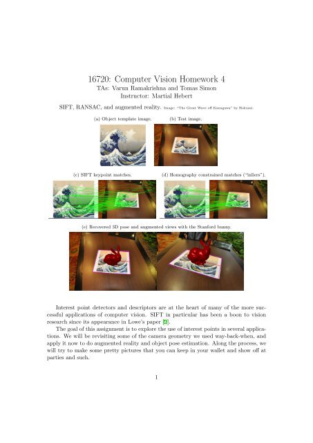
<strong>16720</strong>: <strong>Computer</strong> <strong>Vision</strong> <strong>Homework</strong> 4<br />
TAs: Varun Ramakrishna and Tomas Simon<br />
Instructor: Martial Hebert<br />
SIFT, RANSAC, and augmented reality. Image: “The Great Wave off Kanagawa” by Hokusai.<br />
(a) Object template image.<br />
(b) Test image.<br />
(c) SIFT keypoint matches.<br />
(d) Homography constrained matches (“inliers”).<br />
(e) Recovered 3D pose and augmented views with the Stanford bunny.<br />
Interest point detectors and descriptors are at the heart of many of the more successful<br />
applications of computer vision. SIFT in particular has been a boon to vision<br />
research since its appearance in Lowe’s paper [2].<br />
The goal of this assignment is to explore the use of interest points in several applications.<br />
We will be revisiting some of the camera geometry we used way-back-when, and<br />
apply it now to do augmented reality and object pose estimation. Along the process, we<br />
will try to make some pretty pictures that you can keep in your wallet and show off at<br />
parties and such.<br />
1
1 Harris corners<br />
A simple (and yet very useful 1 ) interest point detector is the Harris corner detector.<br />
Implementing this is quite straightforward and we’d hate for you to miss out on the<br />
opportunity:<br />
For every pixel, we compute the Harris matrix<br />
(∑ ∑ )<br />
Ix I<br />
H = ∑ x<br />
∑ Ix I y<br />
, (1)<br />
Ix I y Iy I y<br />
where the sums are computed over a window in a neighborhood surrounding the<br />
pixel, and will be weighted with a Gaussian window. Remember that this matrix will<br />
be calculated efficiently using convolutions over the whole image. The “cornerness” of<br />
each pixel is then evaluated simply as det(H) − k (trace(H)) 2 (easily vectorized).<br />
Refer to your notes—the algorithm is described in full detail. I also encourage you<br />
to revisit the derivation, it’s really quite beautiful how it all works out in the end.<br />
Figure 1: Harris corners. The importance of scale is apparent in the bottom close-up<br />
views. (Zoom in to see.)<br />
(a) First 500 detected corners (red dots). (b) “Cornerness” heatmap (darker is cornier).<br />
(c) Close-up view, one set of parameters.<br />
(d) Close-up view, a different set.<br />
Q1.1 Discuss the effect of the parameters σ x (the Gaussian sigma parameter used<br />
when calculating image gradients), σ σ ′, (the sigma for th neighborhood window around<br />
1 A cornerstone method, one could say. *groan*<br />
2
each pixel), and k.<br />
Q1.2 Implement your own brand of Harris corner detection. (You can choose the<br />
parameters as you wish, or refer to the paper [1], with k = 0.04 a typical value (empirical)).<br />
Follow the skeleton given in harris.m and p1_script.m. Save the resulting<br />
images as q1_2_heatmap.jpg and q1_2_corners.jpg.<br />
2 SIFT keypoints and descriptor<br />
Because you’d have no time to explore the applications if we ask you to implement<br />
SIFT, we have provided you with Andrea Vedaldi’s implementation of SIFT interest<br />
point detection, and SIFT descriptor computation. This function and many others can<br />
be found in Vedaldi’s (and contributors) excellent VLFeat library [3]. I encourage you to<br />
browse the full package, it has implementations for many computer vision algorithms,<br />
many at the cutting edge of research (for this assignment though, we’ll ask that you only<br />
use the functions provided).<br />
I also suggest—if you’re interested—that you study Lowe’s paper in detail, especially<br />
two concepts that you won’t easily find outside of computer vision: (1) the scale-space,<br />
and (2) using histograms of gradient orientations as a descriptor of a field.<br />
The function is used like this (after doing addpath ./sift):<br />
[keypoints1,descriptors1] = sift( double(rgb2gray(im1))/255, ’Verbosity’, 1 ) ;<br />
Verbosity is not necessary but the function takes a while to compute. (You can save the<br />
results after running once for each image.) See sift_demo.m<br />
3 Image matching, revisited.<br />
This is similar to the approach we followed in homework 2. Instead of using a bank of<br />
filter responses, we will now use the SIFT descriptor as our feature vector, and instead<br />
of computing features per image pixel, we will only compute the features at the scaleinvariant<br />
interest points 2 .<br />
This is going to be a very crude object detector—an objet d’art detector, in fact.<br />
For each training image (in objets/), we will compute SIFT points and descriptors.<br />
Then, for each test image (in images_test/), we will do the same.Because our dataset<br />
is so small, we will directly compare all the test SIFT descriptors with all the training<br />
descriptors for each training image. We will label the testing image as the image with<br />
most.<br />
Q3.1 Write the function [matches, dists]=matchsift(D1, D2,th) that matches<br />
the set of descriptors D1 to D2 (follow the skeleton file given). Use pdist2 to compute<br />
distances. matches is 2 × K where, matches(i, k) is the index in the keypoint array of<br />
image i, of the k-th match or correspondence, for a total of K matches.<br />
2 Sometimes SIFT descriptors are computed densely for every pixel, similarly to homework 2.<br />
3
To make matching a bit more robust, we will implement a commonly heuristic: a<br />
descriptor i in D1 will be said to match j in D2 if the ratio of the distance to the closest<br />
descriptor (call it dist(i, j)) and second-closest descriptor in D2 (call it dist2(i, j)) is<br />
dist(i,j)<br />
smaller than α (i.e.,<br />
dist2(i,j)<br />
≤ α). A common value is α = 0.8. Note: Vedaldi provides<br />
a similar siftmatch function, you can use it to test but you are expected to implement<br />
your own.<br />
Q3.2 For the 6 test images (in images_test/), display the matches side by side<br />
with the training image (in objets/) with most matches, as below. (Use the function<br />
plotmatches(im1, im2, keypoints1, keypoints2, matches), where matches is 2 × N as<br />
above.). Save these images as q3_2_match#.jpg, substituting the testing image number.<br />
Figure 2: SIFT keypoint matches. Image: “Starry night”, from Van Gogh.<br />
4 Homographies, revisited.<br />
In homework 1, we used homographies to create panoramas given two images, but we had<br />
to (tediously) mark the corresponding points manually. Now, with SIFT and RANSAC<br />
in our bag of tricks, we can find these correspondences automatically. Our target application<br />
will be augmented reality—a fancy way of saying that we will embed synthetically<br />
generated elements from a virtual world into real-world images.<br />
The RANSAC algorithm can be applied quite generally to fit any model to data. We<br />
will implement it in particular for (planar) homographies between images:<br />
1. Select a random sample of 4 (tentative) correspondences from the total K (use the<br />
function randsample).<br />
2. Fit a homography to these. (A tentative model.) Use computeH_norm.<br />
3. Evaluate the model on all correspondences. All matches that the model fits with<br />
an error smaller than t make up the “consensus set”. Elements in this set are<br />
called inliers. To determine whether a match fits the model, evaluate the error in<br />
pixels of the projective relation: p 1 ≡ H 2→1 p 2 .<br />
4. If numInliers ≥ d, fit a homography to the consensus set.<br />
4
5. Evaluate the average fitting error on the consensus set. We will use mean distance<br />
between actual and predicted matches, in pixels. If the error is smaller than the<br />
best homography found up till now, update the current best.<br />
Q4.1 Implement RANSAC. The function should have the following fingerprint<br />
[bestH2to1, bestError, inliers]=ransacH2to1(keypoints1, keypoints2, matches).<br />
bestH2to1 should be the homography with least error found during RANSAC, along with<br />
this error bestError. H2to1 will be a homography such that if p 2 is a point in keypoints2<br />
and p 1 is a corresponding point in keypoints1, then p 1 ≡ Hp 2 . inliers will be a vector<br />
of length size(keypoints1,:) with a 1 at those positions that are part of the consensus<br />
set, and 0 elsewhere. We have provided computeH_norm to compute the homography,<br />
but feel free to use your own implementation from homework 1.<br />
Image matching with geometric constraints<br />
In homework 2, you used the spatial pyramid match kernel as a way to use (very coarse)<br />
spatial relations between image features. If a more accurate model of the object is known<br />
(say, it is planar), the geometric constraint that this imposes on the matched features<br />
can be used to reduce false positives.<br />
Q4.2 Create the 6 testing images showing the image with most matches after determining<br />
the set of inliers. Count only inliers as matches this time, and save these images as<br />
q4_1_ransac#.jpg<br />
Figure 3: Keypoint matches after RANSAC with a homography (inliers only).<br />
Note that neither matching nor homography estimation are symmetric. You will<br />
get different results (and different problems) depending on which order you use. Most<br />
common is to match the testing image against the training data, but you can try and<br />
see which one works best.<br />
Augmented reality<br />
Assume that the template image points lie on a 3D plane with Z = 0, and that the<br />
X and Y axes of this 3D plane are aligned with the x and y axes of the image plane.<br />
Thus, the 3D position of our interest points is then P i = (x i − µ x , y i − µ y , 0, 1) T (in<br />
homogeneous coordinates) where x i and y i are the coordinates of the keypoints in the<br />
template image.<br />
5
The vector µ (or mu) is a centering vector given in intrinsics.m, it merely centers<br />
the points such that the origin of the object’s coordinate system lies at the center of the<br />
image. The camera matrix K is also given in intrinsics.m.<br />
Note that you should now recompute your matrix H with the centered points, but<br />
you can use the same inlier set you computed above.<br />
Q4.3 Write the relation between P i and the imaged points in our target image, (u i , v i , 1) T ,<br />
in terms of the camera matrix K, and the camera rotation R and translation t. Use<br />
homogeneous coordinates and projective equivalence.<br />
Q4.4 Write an expression for the columns of a matrix A such that H ≡ KA. This<br />
should be in terms of the rows and/or columns of R and t.<br />
Q4.5 Devise a way to (approximately) recover R and t from H given K. Explain it.<br />
Hint: use the properties of a rotation matrix.<br />
Q4.6 Implement the method you devised in Q2.5 as [R,t]=approxRtFromH(H) where<br />
R is 3 × 3, t is 3 × 1, and H is 3 × 3.<br />
Remember that there are a number of ambiguities that you may need to resolve (e.g.,<br />
the object should face the camera and be in front of it). This can get tricky! You may<br />
want to ignore this issue at first.<br />
Q4.7 Overlay the image axes and the outline of the image onto the picture. (Project<br />
the corresponding object points with your K, R, and t matrices, and plot them.) Save<br />
at least 3 of these images as q4_7_axes#.jpg<br />
Q4.8 Overlay the image axes and the outline of the image onto the picture. Draw<br />
the Stanford bunny landing on the image at the estimated 3D position. (Project the<br />
corresponding object points with your K, R, andt matrices, and plot them, using the<br />
(rotated, translated) Z coordinate now as well. See displaybunny.m). Save at least 3<br />
of these images as q4_7_bunny#.jpg<br />
Figure 4: Estimated pose and bunny augmented image.<br />
Also included is a teapot model, feel free to use that instead, or any other augmentation<br />
that shows that it is working. There are also some extra example images, in case<br />
you want to experiment with more difficult cases, or the creation of other mixed reality<br />
images.<br />
6
Figure 5: Estimated pose and teapot augmented image. Image: Pablo Picasso, La Lectrice<br />
References<br />
[1] C. Harris and M. Stephens. A combined corner and edge detector. In Proceedings of<br />
the 4th Alvey <strong>Vision</strong> Conference, pages 147–151, 1988.<br />
[2] David G. Lowe. Distinctive image features from scale-invariant keypoints. Int. J.<br />
Comput. <strong>Vision</strong>, 60:91–110, November 2004.<br />
[3] A. Vedaldi and B. Fulkerson. VLFeat: An open and portable library of computer<br />
vision algorithms. http://www.vlfeat.org/, 2008.<br />
7