Recognition What Is Recognition?
Recognition What Is Recognition?
Recognition What Is Recognition?

Create successful ePaper yourself
Turn your PDF publications into a flip-book with our unique Google optimized e-Paper software.
<strong>Recognition</strong><br />
Forsyth&Ponce Chap. 22-24<br />
Szeliski Chap. 14<br />
Some of the material from: Fei-Fei Li, Antonio Torralba, Szeliski&Seitz, Rob Fergus<br />
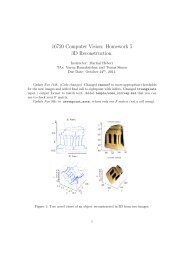
<strong>What</strong> <strong>Is</strong> <strong>Recognition</strong>?<br />
lamp<br />
lamp<br />
phone<br />
vase<br />
keyboard<br />
book<br />
table<br />
building<br />
building<br />
1
Input<br />
Internal Model<br />
Training Example(s)<br />
Output<br />
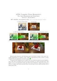
<strong>Recognition</strong>: Simplified story<br />
object 1<br />
Training Images<br />
object m<br />
Features<br />
from<br />
training<br />
image(s)<br />
Features<br />
from input<br />
image<br />
Feature Space<br />
Test image<br />
Approaches based on using feature<br />
matches and geometric relations<br />
Approaches based on classifying/matching<br />
image patches (windows)<br />
2
Example Datasets for<br />
Category <strong>Recognition</strong><br />
Collecting datasets<br />
(towards 10 6-7 examples)<br />
• ESP game (CMU)<br />
Luis Von Ahn and Laura Dabbish 2004<br />
• LabelMe (MIT)<br />
Russell, Torralba, Freeman, 2005<br />
• StreetScenes (CBCL-MIT)<br />
Bileschi, Poggio, 2006<br />
• <strong>What</strong>Where (Caltech)<br />
Perona et al, 2007<br />
• PASCAL challenge<br />
2006, 2007<br />
• Lotus Hill Institute<br />
Song-Chun Zhu et al 2007<br />
• Tiny Images (MIT)<br />
Torralba, Fergus & Freeman 2007<br />
• ImageNet<br />
Fei Fei Li 2009<br />
3
The PASCAL Visual Object<br />
Classes Challenge 2007<br />
The twenty object classes that have been selected are:<br />
Person: person<br />
Animal: bird, cat, cow, dog, horse, sheep<br />
Vehicle: aeroplane, bicycle, boat, bus, car, motorbike, train<br />
Indoor: bottle, chair, dining table, potted plant, sofa, tv/monitor<br />
M. Everingham, Luc van Gool , C. Williams, J. Winn, A. Zisserman 2007<br />
ImageNet (http://www.image-net.org/)<br />
4
Lotus Hill Research Institute image<br />
corpus<br />
Z.Y. Yao, X. Yang, and S.C. Zhu, 2007<br />
Evaluation<br />
5
• Terminology:<br />
– Classification: <strong>Is</strong> the object in the image?<br />
• One-vs.-all<br />
• Forced choice among N<br />
– Detection: <strong>Is</strong> the object in the image and<br />
where?<br />
Correct detection:<br />
• Terminology:<br />
– True positive TP=number of examples<br />
containing the object with object detected<br />
correctly<br />
– True negative TN=number of examples not<br />
containing the object with object not detected<br />
– False positive FP=number of examples not<br />
containing the object with object incorrectly<br />
detected<br />
– True positive FN=number of examples<br />
containing the object with object not detected<br />
6
Precision = TP/(TP+FP)<br />
Out of the detections, how many are correct<br />
ROC curve<br />
Detection<br />
Rate<br />
TP/(TP+FN)<br />
• Most useful in<br />
classification tasks<br />
• Requires TN to be<br />
known<br />
• EER = Equal error rate<br />
= As many false<br />
positives as false<br />
negatives<br />
• AUC = Area under the<br />
curve<br />
False Detections FP or<br />
False detection rate FP/(TN+FP)<br />
Or FPPI = False Positives Per Image<br />
Precision-Recall curve<br />
Recall = TP/(TP+FN)<br />
Same as detection rate for detection tasks<br />
Davis and Goadrich. The Relationship Between Precision-Recall and<br />
ROC Curves. ICML (Intern. Conf. Machine Learning) 2006.<br />
7
Precision-Recall curve<br />
• Invented for retrieval tasks<br />
• Do not need to know TN!<br />
• Summary performance numbers:<br />
– AUPRC = Area under the curve<br />
– AP = Average precision<br />
– F-measure = (1 is perfect performance)<br />
Confusion matrix<br />
• For forced choice classification tasks<br />
• Accuracy = (correct samples)/(total samples)<br />
• Different effect of class imbalance:<br />
– Per-class accuracy<br />
– Total overall accuracy<br />
8
Feature matching<br />
Feature Matching & Geometric<br />
Relations<br />
Features from<br />
training image(s)<br />
Features from<br />
input image<br />
9
Feature Matching & Geometric<br />
Relations<br />
Features from<br />
training image(s)<br />
Features from<br />
input image<br />
Aspect is different between training and test images “invariant” features<br />
Local feature similarity is not sufficient use global geometric consistency<br />
Large number of features define distance in feature space + efficient<br />
indexing<br />
• Image gradients are sampled over 16x16 array of<br />
locations in scale space<br />
• Create array of orientation histograms<br />
• 8 orientations x 4x4 histogram array = 128 dimensions<br />
SIFT<br />
10
Outline<br />
• For each SIFT feature, find the closest<br />
feature in the reference set<br />
• Keep match if distance is greater than<br />
(1+d) times distance to next neighbor<br />
• Apply RANSAC to set of potential<br />
correspondences to verify geometric<br />
consistency<br />
11
Examples<br />
Model: Limited set of<br />
views of the objects<br />
Run-time input:<br />
Object in<br />
arbitrary pose<br />
and illumination<br />
conditions in<br />
uncontrolled<br />
environments<br />
Examples<br />
12
Feature Matching & Geometric<br />
Relations<br />
• Positive:<br />
– Relatively simple implementation<br />
– Well-defined, efficient operations: Indexing, geometric<br />
verification (RANSAC), etc.<br />
• Negative:<br />
– Information reduced to a relatively small set of<br />
discrete features<br />
– Generalization issues for broad categories How do I<br />
deal with recognizing the class of all the chairs?<br />
• Alternative: Use the pixels in the image windows<br />
directly<br />
Window-based techniques<br />
13
Window-based techniques: The<br />
frequency<br />
short story<br />
Example<br />
training window :<br />
feature value<br />
1. Template classification:<br />
Techniques inspired from<br />
template matching:<br />
Compare directly with pixels<br />
from training image.<br />
Perhaps use blurring to be<br />
robust to small shifts, etc.<br />
2. Locally orderless structures:<br />
Intermediate solution: Use<br />
local histograms of features<br />
instead of a single global<br />
histogram. Potentially<br />
combines the advantages of<br />
templates (strong spatial<br />
information) and histograms<br />
(robustness to distortions of<br />
the image)<br />
3. Histograms: Use histograms<br />
of features to compare the<br />
windows. Example: Bags Of<br />
Words techniques.<br />
Problem: All local spatial<br />
information is lost since the<br />
representation is global. Will be<br />
robust to changes but much<br />
less discriminative.<br />
Example from: The Structure of Locally Orderless Images, Jan J. Koenderink AND A. J. Van Doorn, IJCV 1999.<br />
Key approaches: 1. Template<br />
classification<br />
• Nearest-neighbors, PCA, dimensionality<br />
reduction<br />
• Naïve Bayes<br />
• Combination of simple classifiers<br />
(boosting)<br />
• Neural networks<br />
• SVMs<br />
14
Key approaches: 1. Template<br />
classification<br />
• Nearest-neighbors, PCA, dimensionality<br />
reduction<br />
• Naïve Bayes<br />
• Combination of simple classifiers<br />
(boosting)<br />
• Neural networks<br />
• SVMs<br />
Nearest Neighbors<br />
Features<br />
Test image<br />
Feature Space<br />
• Does not require recovery of distributions or decision<br />
surfaces<br />
• Asymptotically twice Bayes risk at most<br />
• Choice of distance metric critical<br />
• Indexing may be difficult<br />
15
Key approaches: 1. Template<br />
classification<br />
• Nearest-neighbors, PCA, dimensionality<br />
reduction<br />
• Naïve Bayes<br />
• Combination of simple classifiers<br />
(boosting)<br />
• Neural networks<br />
• SVMs<br />
More Complicated Features<br />
Scale= 4<br />
Scale = 2<br />
C(x,y,s) =<br />
Wavelet<br />
coefficient at<br />
position x,y at<br />
scale s<br />
Scale 1<br />
• Feature = Set of coefficients S = (C 1 ,..,C N )<br />
Example from Henry Schneiderman<br />
16
• Given features S 1 ,..,S r computed from a<br />
window, threshold the likelihood ratio<br />
P(<br />
S1Sr<br />
log<br />
P(<br />
S S<br />
1<br />
r<br />
| 1)<br />
<br />
)<br />
2<br />
Assume independence<br />
(Naïve Bayes)<br />
P(<br />
S | ) P(<br />
S | ) P(<br />
S | )<br />
log 1 1 log 2 1 ...<br />
log r 1<br />
P(<br />
S | ) P(<br />
S | ) P(<br />
S | )<br />
1 2 2 2<br />
r 2<br />
?<br />
Example from Henry Schneiderman<br />
How can we compute these<br />
probabilities?<br />
Estimating the Probabilities<br />
• Collect the values of the features for training data in<br />
histograms that approximate the probabilities<br />
50-2,000 original images<br />
~1,000 synthetic variations per original image<br />
P (S i | 1 )<br />
S i<br />
~10,000,000 examples<br />
Example from Henry Schneiderman<br />
P (S i | 2 )<br />
S i<br />
17
Compute the values of all the features in the window<br />
For each feature, compute the probabilities of coming from<br />
the object or non-object class<br />
Aggregate into likelihood ratio<br />
From Windows to Images<br />
Search in position<br />
• Move a window to all<br />
possible positions and all<br />
possible scales<br />
• At each (position,scale)<br />
evaluate the classifier<br />
• Return detection if above<br />
threshold<br />
Search in scale<br />
Example from Henry Schneiderman<br />
18
Feature Selection Problem<br />
• Each feature is a set of variables (wavelet<br />
coefficients) S = {C 1 ,..,C N }<br />
• Problem:<br />
– If N is large, the feature is very discriminative<br />
(S is equivalent to the entire window if N is the<br />
total number of variables) but representing the<br />
corresponding distribution is very expensive<br />
– If N is small, the feature is not discriminative<br />
but classification is very fast<br />
Example from Henry Schneiderman<br />
Solution: Classifier Cascade<br />
• Standard problem:<br />
– We can have either discriminative or efficient features<br />
but not both!<br />
– Cannot do classification in one shot<br />
• Standard solution: Classifier Cascade<br />
– Apply first a classifier with simple features Fast and<br />
will eliminate the most obvious non-object locations<br />
– Then apply a classifier with more complex features <br />
More expensive but applied only to these locations<br />
that survived the previous stage<br />
Example from Henry Schneiderman<br />
19
Cascade Example<br />
Cascade Stage 1<br />
Cascade Stage 2<br />
Cascade Stage 3<br />
Apply classifier<br />
with very simple<br />
(and fast) features<br />
Eliminates<br />
most of the image<br />
Apply classifier<br />
with more<br />
complex features<br />
on what is left<br />
Apply classifier<br />
with more<br />
complex features<br />
on what is left<br />
Example from Henry Schneiderman<br />
Cascade Example:<br />
Stage 4<br />
Stage 2<br />
Stage 3<br />
Stage 1<br />
Detection<br />
Rate<br />
False Detections<br />
20
Examples<br />
Key approaches: 1. Template<br />
classification<br />
• Nearest-neighbors, PCA, dimensionality<br />
reduction<br />
• Naïve Bayes<br />
• Combination of simple classifiers<br />
(boosting)<br />
• Neural networks<br />
• SVMs<br />
21
Using Weak Features<br />
abs<br />
x > q ?<br />
Using Weak Features<br />
abs<br />
x > q ?<br />
• Don’t try to design strong features from the beginning,<br />
just use really stupid but really fast features (and a lot of<br />
them)<br />
• Weak learner = Very fast (but very inaccurate) classifier<br />
• Example: Multiply input window by a very simple box<br />
operator and threshold output<br />
(Example from Paul Viola, Distributed by Intel as part of the OpenCV library)<br />
22
Repeat T times<br />
Feature Selection<br />
• Operators defined over all possible shapes and<br />
positions within the window<br />
• For a 24x24 window 45,396 combinations!!<br />
• How to select the “useful” features?<br />
• How to combine them into classifiers?<br />
(Example from Paul Viola)<br />
• Input: Training examples {x i } with labels<br />
(“face” or “non-face” = +/-1) {y i } + weights<br />
w i (initially w i = 1)<br />
• Choose the feature (weak classifier h t ) with<br />
minimum error: e w h ( x ) y<br />
t<br />
• Update the weights such that<br />
– w i is increased if x i is misclassified<br />
– w i is decreased if x i is correctly classified<br />
• Compute a weight a t for classifier h t<br />
– a t large if e t is small<br />
• Final classifier: <br />
i<br />
i<br />
<br />
H(<br />
x)<br />
sgn<br />
<br />
t<br />
i<br />
<br />
t<br />
i<br />
<br />
<br />
a h x <br />
t<br />
t<br />
23
Repeat T times<br />
• Input: Training examples {x i } with labels<br />
(“face” or “non-face”) {y i } + weights w i<br />
(initially w i = 1)<br />
• Choose the feature (weak classifier h t ) with<br />
The training examples that are not<br />
minimum error: e correctly w classified h ( x ) contribute y more<br />
This is a general description of a boosting<br />
algorithm. Well-defined rules for updating w<br />
and for computing a guarantee convergence<br />
and “good” classification performance.<br />
t<br />
• Update the weights such that<br />
– w i is increased if x i is misclassified<br />
– w i is decreased if x i is correctly classified<br />
• Compute a weight a t for classifier h t<br />
– a t large if e t is small<br />
• Final classifier: <br />
H(<br />
x)<br />
sgna<br />
tht<br />
x t <br />
i<br />
<br />
<br />
i t i i<br />
through higher weights<br />
Features that yield good classification<br />
performance receive higher weights<br />
1 st feature selected 2 nd feature selected<br />
The automatic selection process selects “natural” features<br />
(Example from Paul Viola)<br />
24
Detection Rate<br />
Using a Cascade (Again)<br />
• Same problem as before: It is too hard (or impossible) to build a<br />
single accurate classifier<br />
• Key reason: An image containing one face may have 10 5 possible<br />
locations but only 1 “correct” location rare event detection <br />
Would require an enormous number of features<br />
• Solution: Use a cascade of classifiers. Each classifier eliminates<br />
more of the non-object locations while retaining the “object”<br />
locations.<br />
Cascade of 10 20-<br />
feature classifiers<br />
200 feature-classifiers<br />
• In this example, the cascade and the single<br />
classifier have similar accuracy, but the cascade<br />
is 10 times faster<br />
25
Detection Rate<br />
Training: ~5000 face images<br />
+ ~10000 non-face windows<br />
Run-Time: Apply the cascade of<br />
classifiers over all positions and scales<br />
and return those positions/scales that<br />
survive the sequence of classifiers<br />
False Positive Rate<br />
75,081,800 windows scanned over<br />
130 images (507 faces).<br />
(Example from Paul Viola)<br />
26
Window-based techniques: The short story<br />
Training Images object m<br />
object 1<br />
Feature Space<br />
<strong>What</strong> representation should we use?<br />
Test image<br />
Key approaches: 1. Template<br />
classification<br />
• Nearest-neighbors, PCA, dimensionality<br />
reduction<br />
• Naïve Bayes<br />
• Combination of simple classifiers<br />
(boosting)<br />
• Neural networks<br />
• SVMs<br />
27
Neural Networks:<br />
f(x) ~ g(x) (e.g., g(x) = p(o|x))<br />
f<br />
f(x) = orientation of template<br />
sampled at 10 o intervals<br />
f(x) = face detection<br />
posterior<br />
Example from Rowley et al.<br />
28
Convolutional Networks: Lecun et al.<br />
http://yann.lecun.com/exdb/lenet/<br />
Key approaches: 1. Template<br />
classification<br />
• Nearest-neighbors, PCA, dimensionality<br />
reduction<br />
• Naïve Bayes<br />
• Combination of simple classifiers<br />
(boosting)<br />
• Neural networks<br />
• SVMs<br />
29
Example: Pedestrian detection<br />
• Compute the gradients<br />
of the input image in a<br />
detection window<br />
• Compute histograms of<br />
the gradients over 16<br />
directions in overlapping<br />
blocks<br />
• Combine all the<br />
histograms into a single<br />
feature vector f<br />
• Apply a classifier (linear<br />
SVM) trained off-line on<br />
a large training set to f<br />
N. Dalal and B. Triggs . Histograms of Oriented Gradients for Human<br />
Detection. CVPR, 2005<br />
HOG Descriptor = Histogram of<br />
Gradients<br />
Scan input image<br />
Resize<br />
window to<br />
64x128<br />
Divide into<br />
overlapping<br />
16x16<br />
blocks<br />
Compute<br />
histogram<br />
of gradient<br />
over 9<br />
directions<br />
Final feature vector f = 7x15x9 = 945<br />
30
HOG + Linear SVM<br />
Not pedestrian:<br />
W.f < 0<br />
W<br />
HOG Space<br />
Pedestrian:<br />
W.f > 0<br />
Training<br />
31
Histogram of Oriented Gradients (HOG)<br />
• f = vector of gradient histograms<br />
• Input detection window is classified as pedestrian if:<br />
w.f > 0<br />
Example<br />
detection<br />
window<br />
Average<br />
gradients<br />
over the<br />
training data<br />
Positive<br />
components:<br />
Pedestrian<br />
class<br />
Negative<br />
components:<br />
Non-pedestrian<br />
class<br />
N. Dalal and B. Triggs . Histograms of Oriented Gradients for Human Detection. CVPR, 2005<br />
Histogram of Oriented Gradients (HOG)<br />
• f = vector of gradient histograms<br />
• Input detection window is classified as pedestrian if:<br />
w.f > 0<br />
W<br />
Example<br />
detection<br />
window<br />
HOG<br />
descriptor<br />
Positive<br />
components:<br />
Pedestrian<br />
class<br />
Negative<br />
components:<br />
Non-pedestrian<br />
class<br />
N. Dalal and B. Triggs . Histograms of Oriented Gradients for Human Detection. CVPR, 2005<br />
32
Finding the actual detections<br />
Input image +<br />
final detection<br />
Detection confidence<br />
image: Need to find<br />
the local maxima and<br />
suppress the nonlocal<br />
maxima<br />
Examples<br />
33
Other objects<br />
Advanced: How to deal with<br />
geometric deformations?<br />
Coarse model Higherresolution<br />
parts<br />
Model of parts<br />
locations<br />
• A Discriminatively Trained, Multiscale, Deformable Part<br />
Model with Pedro Felzenszwalb and Deva Ramanan, 2008-<br />
2010<br />
34