16720: Computer Vision Homework 1

Instructions
16720: Computer Vision Homework 1
Instructor: Martial Hebert
TAs: Varun Ramakrishna and Tomas Simon
A complete homework submission consists of two parts. A pdf file with answers to the
theory questions and the matlab files for the implementation portions of the homework.
You should submit your completed homework by placing all your files in a directory
named after your andrew id and upload it to your submission directory on Blackboard.
The submission location is the same section where you downloaded your assignment. Do
not include the handout materials in your submission.
All questions marked with a Q require a submission. For the implementation part
of the homework please stick to the function headers described.
Final reminder: Start early! Start early! Start early!. MATLAB is a powerful
and flexible language. It means you can do thins swiftly by a few lines of MATLAB
code; it also means the program may go wrong without reporting any errors. Even for
advanced MATLAB users, it is often the case that a whole day can be spent debugging.
1 Homographies (25 points) (Varun)
In class you have learnt that a homography is an invertible transformation between
points on planes. The homography between planes is a powerful tool that finds use in a
whole bunch of cool applications, some of which you will implement in this assignment.
Let’s begin by exploring the concept of a homography in a little more detail.
1.1 Definition and rank of a homography
Consider two points p and q on planes Π1 and Π2. Let us assume that the homography
that maps point p to q is given by S.
Answer the following questions regarding S:
Q1.1 What is the size (rows x columns) of the matrix S? 1
Q1.2 What is the rank of the matrix S? Explain.
1 Remember to use projective co-ordinates.
p ≡ Sq (1)
1

Q1.3 What is the minimum number of point correspondences (p,q) required to estimate
S? Why?
1.2 Homography between cameras
Q1.4 Suppose we have two cameras C1 and C2 2 viewing a plane Π in 3D space. A
3D point P on the plane Π is projected into the cameras resulting in 2D points u ≡
(x1, y1, 1) and v ≡ (x2, y2, 1). Prove that there exists a homography between the points
u and v.
2 Panoramas (40 points) (Tomas)
We can also use homographies to create a panorama image from multiple views of the
same scene. This is possible for example when there is no camera translation between
the views (e.g., only rotation about the camera center). In this case, corresponding
points from two views of the same scene can be related by a homography 3 :
p i 1 ≡ Hp i 2, (2)
where p i 1 and pi 2 denote the homogeneous coordinates (e.g., pi 1 ≡ (x, y, 1)T ) of the 2D
projection of the i-th point in images 1 and 2 respectively, and H is a 3 × 3 matrix
representing the homography.
2.1 Homography estimation
Q2.1 Given N point correspondences and using (2), derive a set of 2N independent
linear equations in the form Ah = b where h is a 9 × 1 vector containing the unknown
entries of H. What are the expressions for A and b ? How many correspondences will
we need to solve for h?
Q2.2 Implement a function H2to1=computeH(p1, p2). Inputs: p1 and p2 should be
2 x N matrices of corresponded (x, y) T coordinates between two images. Outputs: H
should be a 3x3 matrix encoding the homography that best matches the linear equation
derived above (in the least squares sense). Hint: Remember that H will only be
determined up to scale, and the solution will involve an SVD.
Q2.3 Implement a function H=computeH_norm(p1, p2). This version should normalize
the coordinates p1 and p2 (e.g., from -1 to 1) prior to calling compute_H. Normalization
improves numerical stability of the solution. Note that the resulting H should still follow
Eq. (2). Hint: Express the normalization as a matrix.
2 You can assume that the camera matrices of the two cameras are given by M1 and M2.
3 For an intuition into this relation, consider the projection of point P i = (X, Y, Z) T into two views
p i 1 ≡ KP i and p i 2 ≡ KRP i , where K is a (common) intrinsic parameter matrix, and R is a 3 × 3
rotation matrix. In this case: p i 1 ≡ KR −1 K −1 p i 2.
2

Q2.4 Select enough corresponding points from images taj[1, 2].png using for example
Matlab’s cpselect. They should be reasonably accurate and cover as much of the
images as possible. Use computeH_norm to relate the points in the two views, and plot
image taj1.png with overlayed points p1 (drawn in red), and (drawn in green) points
p2 transformed into the view from image 1 (call this variable p2_t). Save this figure
as q2_4.jpg. Additionally, save these variables to q2_4.mat:
H2to1=computeH_norm(p1,p2);
...
save q2_4.mat H2to1 p1 p2 p2_t;
Write an expression for the average error (in pixels) between p1 and the transformed
points p2. This expression should be in terms of H, p1, and p2. Compare this to the
error that was minimized in items 1 and 2.
2.2 Image warping
The provided function warp_im=warpH(im, H, out_size) warps image im using the
homography transform H. The pixels in warp_im are sampled at coordinates in the rectangle
(1, 1) to (out_size(2), out_size(1)). The coordinates of the pixels in the source
image are taken to be (1, 1) to (size(im,2), size(im,1)) and transformed according to
H.
The following code:
H2to1=computeH_norm(p1,p2);
warp_im=warpH(im2, H2to1, size(im1));
should produce a warped image im2 in the reference frame of im1. Not all of im2 may
be visible, and some pixels may not be drawn to.
Figure 1: Original images and warped.
(a) taj1.jpg (b) taj2.jpg (c) taj2 warped into taj1
Q2.5 Write a few lines of Matlab code to find a matrix M, and out_size in terms of
H2to1 and size(im1) and size(im2) such that,
warp_im1=warpH(im1, M, out_size);
warp_im2=warpH(im2, M*H2to1, out_size);
3

produces images in a common reference frame where all points in im1 and im2 are
visible (a mosaic or panorama image containing all views) and out_size(2)==1280.
M should be scaling and translation only, and the resulting image should fit snugly
around the transformed corners of the images.
2.3 Image blending
Figure 2: Final mosaic view.
Q2.6 Use the functions above to produce a panorama or mosaic view of the two images,
and show the result. Save this image as q2_7.jpg. For overlapping pixels, it
is common to blend between the values of both images. You can simply average the
values. Alternatively, you can obtain a blending value for each image:
mask = zeros(size(im,1), size(im,2));
mask(1,:) = 1; mask(end,:) = 1; mask(:,1) = 1; mask(:,end) = 1;
mask = bwdist(mask, ’city’);
mask = mask/max(mask(:));
The function bwdist computes the distance transform of the binarized input image, so
this mask will be zero at the borders and 1 at the center of the image.
Q2.7 In items Q2.1−2.3 we solved for the 8 degrees of freedom of a homography. Given
that the two views were taken from the same camera and involve only a rotation, how
might you reduce the number of degrees of freedom that need to be estimated?
QX1 (Extra Credit 10 points) Assume that the rotation between the cameras is
only around the y axis. Using H2to1, and assuming 4 no skew and α = β = 1274.4,
4 The previous notation used α = fx, β = fy, u0 = cx, v0 = cy, and no skew.
4

u0 = 814.1, and v0 = 526.6, estimate the angle of rotation between the views. You
should be able to approximate this with elementary trigonometry.
2.4 Extra credit: Laplacian pyramid blending
Linear blending produces ghosting artifacts when the scene changes between the views
(e.g., the people in the example images). In these regions, we should take the pixels
from only one image. Unfortunately, having hard seams between images often introduces
noticeable discontinuities, as for example an abrupt change in the color of the sky.
Laplacian blending alleviates this problem by blending features at different frequency
bands.
QX2 (Extra Credit 10 points) Implement laplacian pyramid blending for images.
First construct a gaussian pyramid of each image and mask. Then, construct the laplacian
pyramid using the difference of gaussians. Now blend each of the levels together
with the corresponding mask, and reconstruct the image. Show your impressive results.
Figure 3: An Annoying Clockwork Orange.
(a) oranges.jpg (b) alex.jpg (c) mask.jpg
(d) Gaussian and laplacian pyramids.
5
(e) Blended result, normal (top),
and 5-level pyramid (bottom).

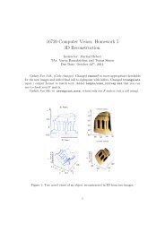
3 Camera Estimation (35 points) (Varun)
In class we learnt that the camera matrix M can be decomposed into its intrinsic parameters
given by the matrix K and extrinsic parameters given by the rotation R and
translation t
M = K [R t] (3)
and the camera projection equation is given by:
p ≡ MP (4)
The rotation and translation of the camera is also commonly referred to as the pose
of the camera. A problem that commonly arises in areas such as model-based object
recognition, augmented reality and vision-based robot navigation is that of estimating
the pose of the camera given 3D co-ordinates of points on an object/scene and their
corresponding 2D projections in the image. In this question we shall explore the use of
pose estimation in a problem that arises in motion capture.
3.1 Problem Statement
Given the locations of 3D optical markers placed at the joints of a human subject, and
the corresponding locations of the markers in the image, estimate the pose of the camera
relative to the human subject.
Begin by loading the file hw1 prob3.mat into your matlab workspace. You will find
two variables in your workspace:
• xy - a 23 × 2 matrix of the 2D locations of the joints in the image
• XYZ - a 23 × 3 matrix of the 3D locations of the joint markers in the scene.
For this assignment the 2D image points and the 3D joint marker positions have
been generated synthetically, we will first visualize our data (First rule of implementing
a computer vision algorithm- visualize, visualize, visualize). You have been given two
functions visualize2Dpoints and visualize3Dpoints 5 to help you with this.
3.2 Estimating the camera
Q3.1 Your primary task in this problem is to write the following function and answer
the questions that follow:
[R, t] = estimateCamera(xy, XYZ)
5 Type ’help functionname’ in matlab to get information on usage.
6

which takes as input the 23 × 2 matrix xy of 2D locations and the 23 × 3 matrix of
3D locations XY and returns as output the rotation R and translation t of the camera
in the object co-ordinate system. We will assume that the camera intrinsic parameter
matrix K is given and is equal to the identity matrix.
The camera matrix M that you estimated needs to be separated into a rotation R
and a translation t.
Q3.2 You could imagine simply taking the first 3 × 3 part of M to be the rotation of
the camera. However, this would be incorrect, explain why.
Q3.3 Under what condition is the 3 × 3 matrix a rotation matrix ?
Q3.4 How can we convert the first 3 × 3 portion of the matrix M into a rotation
matrix? 67
Q3.5 Write the following function by making the change you derived in the previous
question to correct the camera estimate
[R,t] = estimateCamera2(xy, XYZ)
3.3 Visualization
Q3.6 Visualize the given 3D joint marker points using the provided visualize3Dpoints
function and place the estimated camera in the scene using the provided drawCam
function.
3.4 Epilogue
In this problem we have implemented a simple version of pose estimation which might
not very stable for real applications. There are several current state of the art approaches
for estimating the perspective camera pose from 2D-3D correspondences (also known as
the Perspective-N-Points problem), such as in the following paper:
EPnP: Accurate O(n) Solution to the PnP Problem - Francesc Moreno-
Noguer, Vincent Lepetit, Pascal Fua. (IJCV 2008)
Change log
Sept. 11th: Revised grading scheme to be Problem 1: 25 points, Problem 2: 40 points,
problem 3: 35 points.
Sept. 11th: Changed notation in QX1 to match what was used in class.
6 This estimate will actually be the best rotation in a least-squares sense.
7 Hint: The solution uses an SVD.
7

10
5
0
−5
−10
−15
0
10
20
30
40
50
4
2
0
−2
Figure 4: Human skeleton visualization with estimated camera position.
8