Cutting Error Prediction by Multilayer Neural Networks for Machine ...

Cutting Error Prediction by Multilayer Neural Networks
for Machine Tools with Thermal Expansion and
Compression
Kenji NAKAYAMA Akihiro HIRANO Shinya KATOH
Tadashi YAMAMOTO† Kenichi NAKANISHI† Manabu SAWADA†
Dept of Information and Systems Eng., Faculty of Eng., Kanazawa Univ.
2–40–20 Kodatsuno, Kanazawa, 920–8667, Japan
e-mail: nakayama@t.kanazawa-u.ac.jp
† Nakamura-Tome Precision Industry Co., Ltd.
Abstract
In training neural networks, it is important to reduce
input variables for saving memory, reducing network
size, and achieving fast training. This paper proposes
two kinds of selecting methods for useful input variables.
One of them is to use information of connection weights
after training. If a sum of absolute value of the connection
weights related to the input node is large, then
this input variable is selected. In some case, only positive
connection weights are taken into account. The
other method is based on correlation coefficients among
the input variables. If a time series of the input variable
can be obtained by amplifying and shifting that of
another input variable, then the former can be absorbed
in the latter. These analysis methods are applied to predicting
cutting error caused by thermal expansion and
compression in machine tools. The input variables are
reduced from 32 points to 16 points, while maintaining
good prediction within 6µm, which can be applicable to
real machine tools.
1 Introduction
Recently, prediction and diagnosis have been very important
in a real world. In many cases, relations between
the past data and the prediction, and the symptoms and
diseases are complicated nonlinear. Neural networks are
useful for these signal processing. Many kinds of approaches
have been proposed [1]–[12].
In these applications, observations, which are the
past data, the symptoms and so on, are applied to the
input nodes of neural networks, and the prediction and
the diseases are obtained at the network outputs. In order
to train neural networks and to predict the coming
phenomenon and to diagnose the diseases, it should be
analyzed what kinds of observations are useful for these
purposes. Usually, the observations, which seems to be
meaningful by experience, are used. In order to simplify
observation processes, to minimize network size, and to
make a learning process fast and stable, the input data
should be minimized. How to selected the useful input
variables have been discussed [11]–[12].
In this paper, selecting methods for useful input
variables are proposed. The corresponding connection
weights and correlation coefficients among the input
data are used. The proposed methods are applied to
predicting cutting error caused by thermal expansion
and compression in numerical controlled (NC) machine
tools. Temperature is measured at many points on the
machine tool and in the surroundings. For instance, 32
points are measured, which requires a complicated observation
system. It is desirable to reduce the temperature
measuring points.
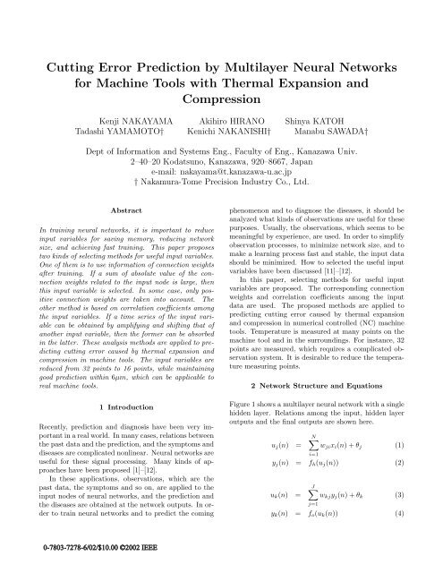
2 Network Structure and Equations
Figure 1shows a multilayer neural network with a single
hidden layer. Relations among the input, hidden layer
outputs and the final outputs are shown here.
u j (n) =
N∑
w ji x i (n)+θ j (1)
i=1
y j (n) = f h (u j (n)) (2)
u k (n) =
J∑
w kj y j (n)+θ k (3)
j=1
y k (n) = f o (u k (n)) (4)
0-7803-7278-6/02/$10.00 ©2002 IEEE

x 1(n)
wj i
w k j
the important input variables are selected by using a
sum of the corresponding connection weights after the
training.
y (n) k
J∑
S i,abso = |w ji | (12)
j=1
x N(n)
Input layer
+1
θj
y j
Hidden layer
(n)
θk
Output layer
Figure 1: Multilayer neural network with a single hidden
layer.
f h () and f o () are sigmoid functions. The connection
weights are trained through supervised learning algorithms,
such as an error back-propagation algorithm.
3.2 Method-Ib: Based on Positive Connection
Weights
When the input data always take positive numbers, negative
connection weights may reduce the input potential
u j (n) in Eq.(1). Furthermore, when a sigmoid function
shown in Fig.2 is used for an activation function, negative
u j (n) generates small output, which does not affect
the final output. Thus, in this case, the negative connection
weights are not useful. Therefore, only positive
connection weights are taken into account. The useful
temperatures are selected based on S i,posi .
S i,posi = ∑ σ
w σi , w σi > 0 (13)
3 Analysis Methods for Useful Input Data
3.1 Method-Ia: Based on Absolute Value of
Connection Weights
The connection weights are updated following the error
back-propagation (BP) algorithm. f˙
o () and f ˙ h () are the
1st order derivative of f o () and f h (), respectively.
w kj (n +1) = w kj (n)+∆w kj (n) (5)
∆w kj (n) = α∆w kj (n − 1)+ηδ k y j (n) (6)
δ k = e k (n) f ˙ o (u k (n)) (7)
e k (n) = d k (n) − y k (n), d k (n) is a target.(8)
w ji (n +1) = w ji (n)+∆w ji (n) (9)
∆w ji (n) = α∆w ji (n − 1)+ηδ j x i (n) (10)
δ j = f ˙
K∑
h (u j (n)) δ k w kj (n) (11)
k=1
From the above equations, the connection weight w ji (n)
is updated by ηδ j x i (n). Since η is usually a positive
small number, then by repeating the updating, ηδ j x i (n)
is accumulated in w ji (n+1). Thus, growth of w ji (n+1)
is expressed by E[δ j x i (n)], which is a cross-correlation.
On the other hand, as shown in Eq.(11), δ j expresses
the output error caused by the jth hidden unit output.
If the input variable x i (n) is an important factor, then
it may be closely related to the output error, and their
cross-correlation becomes a large value. For this reason,
it can be expected that the connection weights for the
important input variables to the hidden units will be
grown up in a learning process. Based on this analysis,
f (u)
0 u
Figure 2: Sigmoid function, whose output is always positive.
3.3 Method II: Based on Cross-correlation
among Input variables
Dependency among Input variables
First, we discuss using a neuron model shown in Fig.3.
The input potential u is given by
w1
x1
y = f(u )
w2
x2
u
α
1 (bias)
Figure 3: Neuron model.
u = w 1 x 1 + w 2 x 2 + α (14)
0-7803-7278-6/02/$10.00 ©2002 IEEE

If the following linear dependency is held,
x 2 = ax 1 + b a and b are constant (15)
then, u is rewrriten as follows:
u = w 1 x 1 + w 2 (ax 1 + b)+α (16)
= (w 1 + aw 2 )x 1 +(bw 2 + α) (17)
(18)
Therefore, by replacing w 1 by w 1 +aw 2 and α by bw 2 +α,
the input variable x 2 can be removed as follows:
u = wx 1 + β (19)
w = w 1 + aw 2 (20)
β = bw 2 + α (21)
This is an idea behind the proposed analysis method.
The linear dependency given by Eq.(15) can be analyzed
by using correlation coefficients.
Correlation Coefficients
The ith input variable is defined follows:
x i =[x i (0),x i (1), ··· ,x i (L − 1)] T (22)
Correlation coefficient between the ith and the jth variable
vectors is given by
(x i − ¯x i ) T (x j − ¯x j )
ρ ij =
(23)
‖ x i − ¯x i ‖‖ x j − ¯x j ‖
¯x i,j = 1 L−1
∑
x i,j (n) (24)
L
n=0
If x i and x j satisfy Eq.(15), then ρ ij = 1. In other
words, if ρ ij is close to unity, then x i and x j are linearly
dependent. On the other hand, if ρ ij = 0, then they are
orthogonal to each other.
Combination of Data Sets
The modifications by Eqs.(19)–(21) are common in a
MLNN. This means the modifications are the same for
all the input data sets. Let the number of the data sets
be Q. The input variables are re-defined as follows:
Definition of Input Data for Q Data Sets
x (q)
i
= [x (q)
i
(0),x (q)
i
(1), ··· ,x (q)
i
(L − 1)] T (25)
X (q) = [x (q)
1 , x(q) 2 , ··· , x(q)
N
⎡
] (26)
X (1) ⎤
X (2)
X total = ⎢ ⎥
⎣ . ⎦ =[˜x 1, ˜x 2 , ··· , ˜x N ] (27)
˜x i =
⎡
⎢
⎣
X (Q)
x (1)
i
x (2)
ị
.
x (Q)
i
⎤
⎥
⎦
(28)
is the input variable vector of the qth input data set.
X (q) is the qth input data set, X total is a total input
data set, which includes all the input data. In ˜x i , the
ith variables at all sampling points, n =0, 1, ··· ,L− 1
and for all data sets q =1, 2, ··· ,Q are included. Using
these notations, the correlation coefficients are defined
as follows:
x (q)
i
ρ ij =
¯˜x i =
(˜x i − ¯˜x i ) T (˜x j − ¯˜x j )
‖ ˜x i − ¯˜x i ‖‖ ˜x j − ¯˜x j ‖
(29)
1
Q∑
L−1
∑
x (q)
i (n)
LQ
(30)
q=1 n=0
One example of the combined input data is shown in
Fig.4, where Q =4.
data set 1 data set 2 data set 3 data set 4
4L
ρij
Figure 4: Combined input variable vectors.
Aberage of Correlation Coefficients
Method-IIa
The correlation coefficients for all combinations of the
input variables are calculated by Eq.(29). Furthermore,
dependency of the ith variable is evaluated by
¯ρ (1)
i
¯ρ (1)
i
= 1
N − 1
N∑
ρ ij (31)
j=1
̸=i
expresses average of the correlation coefficients between
the ith variable and all the other variables. Thus,
the variables, which have small ¯ρ i are selected for the
useful input variables.
Method-IIb
Let x σ be the selected variable vectors, and the number
of x σ be N 1 . The correlation coefficients ρ (2)
ij are
evaluated once more among the selected σ variable vectors.
The variable vectors are further selected based on
ρ (2)
ij . The variables having large ρ(2) ij are removed from
the selected set. Instead, the variables, which are not
selected in Method-IIa and have small ¯ρ (1)
i
, are selected
and added to x σ . This process is repeated until all the
selected variables have small ρ (2)
ij .
0-7803-7278-6/02/$10.00 ©2002 IEEE

3.4 Comparison with Other Analysis Methods
There are several methods to extract important components
among the input data. One of them is principal
component analysis. The other method is vector
quantization. In these methods, however, in order to
extract these components and vectors, many input data
are required. Our purpose is to simplify the observation
process for the input data, that is to select useful input
variables, which are directly observed. It is difficult
to obtain the useful observation data from the principal
components and the representative vectors.
4 Prediction of Cutting Error Caused by
Thermal Expansion and Compression
Numerical controlled (NC) machine tools are required
to guarantee very high cutting precision, for instance
tolerance of cutting error is within 10µm in diameter.
There are many factors, which degrade cutting precision.
Among them, thermal expansion and compression
of machine tools are very sensitive in cutting precision.
In this paper, the multilayer neural network is applied
to predicting cutting error caused by thermal effects.
4.1 Structure of NC Machine Tool
Figure 5 shows a blockdiagram of NC machine tool.
Distance between the cutting tool and the objective
is changed by thermal effects. Temperatures at many
Index
Cutting Tool
Frame ( front, back )
z
x
X Axis Slide
dependent on hysteresis of temperature change. x i (n)
means the temperature at the ith measuring point and
at the nth sampling points on the time axis. Its delayed
samples x i (n − 1),x i (n − 2), ··· are generated through
the delay elements ”T” and are applied to the MLNN.
One hidden layer and one output unit are used.
x
x
Delay
x
1(n-1)
1(n-l+1)
1(n)
N(n)
T
T
x
N
x
T
T
(n-l+1)
w
j i
Hidden layer
w
j
y
j (n)
Output layer
e(n)
+
-
y (n)
Figure 6: Neural network used for predicting cutting error
caused by thermal effects.
4.3 Training and Testing Using All Input variables
Four kinds of data sets are measured by changing cutting
conditions. They are denoted D 1 ,D 2 ,D 3 ,D 4 . Since
it is not enough to evaluate prediction performance of
the neural network, data sets are increased by combining
the measured data sets by linear interpolation, denoted
D 12 ,D 13 ,D 14 ,D 23 ,D 24 ,D 34 . Some of the measured
temperatures in time are shown in Fig.7. Training
and testing conditions are shown in Table 1. All measuring
points are employed. The data sets except for D 1
are used for training and D 1 is used for testing.
Figure 8 shows a learning curve using all data sets,
d(n)
Head Stock
55
Z Axis Slide
Objective
50
Figure 5: Rough sketch of NC machine tool.
points on the machine tool and in surrounding are measured.
The number of measuring points is up to 32
points.
4.2 Multilayer Neural Network
Figure 6 shows the multilayer neural network used predicting
cutting error of machine tools. The temperature
and deviation are measured as a time series. Thermal
expansion and compression of machine tools are also
Temperature [ C ]
45
40
35
30
25
20
0 5 10 15 20 25 30 35 40 45 50
Time [ min ]
Figure 7: Some of measured temperatures in time.
0-7803-7278-6/02/$10.00 ©2002 IEEE

Table 1: Training and testing conditins
Measuring points
32 points
Training data sets D 2 ,D 3 ,D 4
D 12 ,D 13 ,D 14 ,D 23 ,D 24 ,D 34
Test data set D 1
Learning rate η 0.001
Momentum rate α 0.9
Iterations 100,000
5.1 Selection Based on Connection Weights
The measuring points are selected based on a sum of absolute
value of the connection weights S i,abso (Method-
Ia) and on a sum of positive connection weights S i,posi
(Method-Ib). Figure 10 shows both sums. The horizontal
axis shows the temperature measuring points, that
is 32 points. Their prediction are shown in Fig.11. The
selection method using S i,posi is superior to the other using
S i,abso , because the temperature in this experience
is always positive. The prediction error is within 6µm.
except for D 1 , and all measuring points, that is 32
points. The vertical axis means the mean squared error
(MSE) of difference between the measured cutting error
and the predicted cutting error. It is well reduced.
12
10
Sum of Absolute Value
Sum of Positive Value
8
0.002
6
0.0015
4
2
MSE
0.001
0
1 2 3 4 5 6 7 8 9 10 11 12 13 14 15 16 17 18 19 20 21 22 23 24 25 26 27 28 29 30 31 32
0.0005
Figure 10: Sum of absolute value of temperature and positive
temperature.
0
0 10000 20000 30000 40000 50000 60000 70000 80000 90000 100000
iteration
Figure 8: Learning curve of cutting error prediction. All
measuring points are used.
Figure 9 shows cutting error prediction under the conditions
in Table 1. The prediction error is within 6µm,
which satisfies the tolerance 10µm in diameter.
Deviation [ µm ]
8
4
0
-4
-8
-12
-16
Sum of Absolute Value
Sum of Positive Value
Measurement
Deviation [ µm ]
8
4
0
-4
-8
-12
-16
-20
Prediction
Measurememt
-20
-24
-28
-32
0
250 500 750 1000 1250 1500
Time [ min ]
Figure 11: Cutting error prediction with 16 measuring
points selected by connection weights.
-24
-28
0
250 500 750 1000 1250 1500
Time [ min ]
Figure 9: Cutting error prediction. All measuring points
are used.
5 Selection of Useful Measuring Points
The useful 16 measuring points are selected from 32
points by the analysis methods proposed in Sec.3.
5.2 Selection Based on Correlation Coefficients
In Method-IIb, after the first selection by Method-IIa,
the variables, whose correlation coefficients ρ (2)
ij exceed
0.9 are replaced by the variables, which are not selected
in the first stage and have small ¯ρ (1)
i . Simulation results
by both methods are shown in Fig.12. The result
by Method-IIb ”Correlation(2)” is superior to that of
Method-IIa ”Correlation(1)”. Because the former more
precisely evaluates the correlation coefficients.
0-7803-7278-6/02/$10.00 ©2002 IEEE

Deviation [ µm ]
12
8
4
0
-4
-8
-12
-16
-20
-24
-28
0
Correlation (1)
Correlation (2)
Measurement
250 500 750 1000 1250 1500
Time [ min ]
Figure 12: Cutting error prediction with 16 measuring
points selected by correlation coefficients.
5.3 Comparison of Selected Measuring Points
Table 2 shows the selected temperature measuring
points by four kinds of the methods. Comparing the
selected measuring points by Method-Ib and Method-
IIb, the following 9 points 4, 11, 12, 14, 15, 21, 22, 28, 31
are common. However, the selected measuring points
are not exactly the same. A combination of the measuring
points seems to be important.
Table 2: Measuring points selected by four kinds of methods.
Methods
Measuring points
Method-Ia 2, 3, 6, 7, 9,15,18,19,
Sum of absolute values 21,22,24,25,26,28,30,31
Method-Ib 1, 4, 7, 9, 11,12,13,14,
Sum of positive weights 15,19,21,22,23,26,28,31
Method-IIa 3, 4, 7, 8,12,14,16,18,
Correlation(1) 19,20,21,22,23,25,31,32
Method-IIb 3, 4, 8,11,12,14,15,16,
Correlation(2) 20,21,22,27,28,30,31,32
6 Conclutions
Two kinds of methods, selecting the useful input variables,
have been proposed. They are based on the connection
weights and the correlation coefficients among
the input variables. The proposed methods have been
applied to predicting cutting error caused by thermal
effects in machine tools. Simulation results show precise
prediction with the reduced number of the input
variables.
References
[1] S.Haykin, ”Neural Networks: A Comprehensive
Foundation,” Macmillan, New York, 1994.
[2] S.Haykin and L. Li, ”Nonlinear adaptive prediction
of nonstationary signals,” IEEE Trans. Signal Processing,
vol.43, No.2, pp.526-535, Feburary. 1995.
[3] A. S. Weigend and N. A. Gershenfeld, ”Time series
prediction: Forecasting the future and understanding
the past. in Proc. V. XV, Santa Fe Institute, 1994.
[4] M. Kinouchi and M. Hagiwara, ”Learning temporal
sequences by complex neurons with local feedback,”
Proc. ICNN’95, pp.3165-3169, 1995.
[5] T.J. Cholewo and J.M. Zurada, ”Sequential network
construction for time series prediction,” in Proc.
ICNN’97, pp.2034-2038, 1997.
[6] A. Atia, N. Talaat, and S. Shaheen, ”An efficient
stock market forecasting model using neural networks,”
in Proc. ICNN’97, pp.2112-2115, 1997.
[7] X.M. Gao, X.Z. Gao, J.M.A. Tanskanen, and S.J.
Ovaska, ”Power prediction in mobile communication
systems using an optimal neural-network structure”,
IEEE Trans. on Neural Networks, vol.8, No.6, pp.1446-
1455, November 1997.
[8] A.A.M.Khalaf, K.Nakayama, ”A cascade form
predictor of neural and FIR filters and its minimum size
estimation based on nonlinearity analysis of time series”,
IEICE Trans. Fundamental, vol.E81-A, No.3, pp.364–
373, March 1998.
[9] A.A.M.Khalaf, K.Nakayama, ”Time series prediction
using a hybrid model of neural network and FIR
filter”, Proc. of IJCNN’98, Anchorage, Alaska, pp.1975-
1980, May 1998.
[10] A.A.M. Khalaf and K.Nakayama, ”A hybrid nonlinear
predictor: Analysis of learning process and
predictability for noisy time series”, IEICE Trans.
Fundamentals,Vol.E82-A, No.8, pp.1420-1427, Aug.
1999.
[11] K.Hara and K.Nakayama, ”Training data selection
method for generalization by multilayer neural networks”,
IEICE Trans. Fundamentals, Vol.E81-A, No.3,
pp.374-381, March 1998.
[12] K.Hara and K.Nakayama, ”A training data selection
in on-line training for multilayer neural networks”,
IEEE–INNS Proc. of IJCNN’98, Anchorage, pp.227-
2252, May 1998.
0-7803-7278-6/02/$10.00 ©2002 IEEE