Q Factor Measurements with an SWR Meter - Ve2azx.net
Q Factor Measurements with an SWR Meter - Ve2azx.net
Q Factor Measurements with an SWR Meter - Ve2azx.net

You also want an ePaper? Increase the reach of your titles
YUMPU automatically turns print PDFs into web optimized ePapers that Google loves.
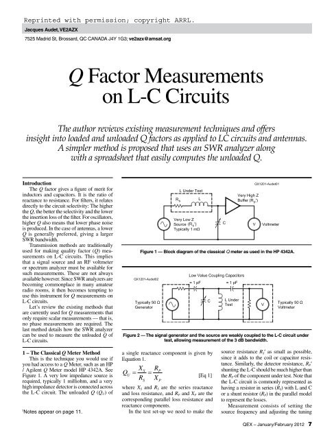
Jacques Audet, VE2AZX<br />
7525 Madrid St, Brossard, QC CANADA J4Y 1G3; ve2azx@amsat.org<br />
Q <strong>Factor</strong> <strong>Measurements</strong><br />
on L-C Circuits<br />
The author reviews existing measurement techniques <strong>an</strong>d offers<br />
insight into loaded <strong>an</strong>d unloaded Q factors as applied to LC circuits <strong>an</strong>d <strong>an</strong>tennas.<br />
A simpler method is proposed that uses <strong>an</strong> <strong>SWR</strong> <strong>an</strong>alyzer along<br />
<strong>with</strong> a spreadsheet that easily computes the unloaded Q.<br />
Introduction<br />
The Q factor gives a figure of merit for<br />
inductors <strong>an</strong>d capacitors. It is the ratio of<br />
react<strong>an</strong>ce to resist<strong>an</strong>ce. For filters, it relates<br />
directly to the circuit selectivity: The higher<br />
the Q, the better the selectivity <strong>an</strong>d the lower<br />
the insertion loss of the filter. For oscillators,<br />
higher Q also me<strong>an</strong>s that lower phase noise<br />
is produced. In the case of <strong>an</strong>tennas, a lower<br />
Q is generally preferred, giving a larger<br />
<strong>SWR</strong> b<strong>an</strong>dwidth.<br />
Tr<strong>an</strong>smission methods are traditionally<br />
used for making quality factor (Q) measurements<br />
on L-C circuits. This implies<br />
that a signal source <strong>an</strong>d <strong>an</strong> RF voltmeter<br />
or spectrum <strong>an</strong>alyzer must be available for<br />
such measurements. These are not always<br />
available however. Since <strong>SWR</strong> <strong>an</strong>alyzers are<br />
becoming commonplace in m<strong>an</strong>y amateur<br />
radio rooms, it then becomes tempting to<br />
use this instrument for Q measurements on<br />
L-C circuits.<br />
Let’s review the existing methods that<br />
are currently used for Q measurements that<br />
only require scalar measurements — that is,<br />
no phase measurements are required. The<br />
last method details how the <strong>SWR</strong> <strong>an</strong>alyzer<br />
c<strong>an</strong> be used to measure the unloaded Q of<br />
L-C circuits.<br />
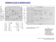
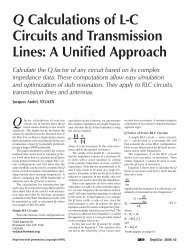
Figure 1 — Block diagram of the classical Q meter as used in the HP 4342A.<br />
Figure 2 — The signal generator <strong>an</strong>d the source are weakly coupled to the L-C circuit under<br />
test, allowing measurement of the 3 dB b<strong>an</strong>dwidth.<br />
1 – The Classical Q <strong>Meter</strong> Method<br />
This is the technique you would use if<br />
you had access to a Q <strong>Meter</strong>, such as <strong>an</strong> HP<br />
/ Agilent Q <strong>Meter</strong> model HP 4342A. See<br />
Figure 1. A very low imped<strong>an</strong>ce source is<br />
required, typically 1 milliohm, <strong>an</strong>d a very<br />
high imped<strong>an</strong>ce detector is connected across<br />
the L-C circuit. The unloaded Q (Q U ) of<br />
1<br />
Notes appear on page 11.<br />
a single react<strong>an</strong>ce component is given by<br />
Equation 1.<br />
Q<br />
X<br />
R<br />
= S P<br />
U<br />
R<br />
= S<br />
X<br />
[Eq 1]<br />
P<br />
where X S <strong>an</strong>d R S are the series react<strong>an</strong>ce<br />
<strong>an</strong>d loss resist<strong>an</strong>ce, <strong>an</strong>d R P <strong>an</strong>d X P are the<br />
corresponding parallel loss resist<strong>an</strong>ce <strong>an</strong>d<br />
react<strong>an</strong>ce components.<br />
In the test set-up we need to make the<br />
source resist<strong>an</strong>ce R S ′ as small as possible,<br />
since it adds to the coil or capacitor resist<strong>an</strong>ce.<br />
Similarly, the detector resist<strong>an</strong>ce, R P ′<br />
shunting the L-C should be much higher th<strong>an</strong><br />
the R P of the component under test. Note that<br />
the L-C circuit is commonly represented as<br />
having a resistor in series (R S ) <strong>with</strong> L <strong>an</strong>d C<br />
or a shunt resistor (R P ) in the parallel model<br />
to represent the losses.<br />
Measurement consists of setting the<br />
source frequency <strong>an</strong>d adjusting the tuning<br />
QEX – J<strong>an</strong>uary/February 2012 7
capacitor, C, for reson<strong>an</strong>ce to maximize the<br />
voltage across the resonating capacitor C.<br />
The Q is calculated using Equation 2.<br />
Voltage Across C<br />
Q =<br />
Source Voltage<br />
[Eq 2]<br />
Note that the source voltage is in the<br />
millivolt r<strong>an</strong>ge, since it will be multiplied by<br />
the Q factor. A 10 mV source <strong>an</strong>d a Q of 500<br />
will give 5 V across the L-C circuit. In order<br />
to preserve the high imped<strong>an</strong>ce of the detector<br />
even at the higher frequencies, a capacitive<br />
voltage divider is used.<br />
This circuit measures the unloaded Q<br />
called Q U provided that the series resist<strong>an</strong>ce<br />
R S of the inductor under test is much higher<br />
th<strong>an</strong> the source resist<strong>an</strong>ce R S ′ <strong>an</strong>d the detector<br />
parallel resist<strong>an</strong>ce R P ′ is much larger th<strong>an</strong> the<br />
L-C circuit R P . 1<br />
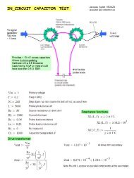
2 – Tr<strong>an</strong>smission Method Using<br />
Coupling Capacitors<br />
A signal is coupled into <strong>an</strong> L-C parallel<br />
circuit using a low value capacitor <strong>an</strong>d<br />
extracts the output signal using the same<br />
value of capacitor. 2 See Figure 2. Note that<br />
inductive coupling is also possible, as used in<br />
tr<strong>an</strong>smission line (cavity) resonators.<br />
The – 3 dB b<strong>an</strong>dwidth (BW) is measured<br />
at the reson<strong>an</strong>t frequency f 0 , <strong>an</strong>d the loaded Q<br />
(Q L ) is calculated <strong>with</strong> Equation 3.<br />
f0<br />
QL<br />
= [Eq 3]<br />
BW<br />
The obtained b<strong>an</strong>dwidth, BW, is a function<br />
of the coupling, <strong>an</strong>d <strong>an</strong>other calculation<br />
is required to get Q U , the unloaded Q. When<br />
the input to output coupling is identical, we<br />
use Equation 4.<br />
⎛ Q ⎞<br />
U<br />
Loss = 20 log⎜ ⎟ [Eq 4]<br />
⎝ QU<br />
−QL<br />
⎠<br />
where Loss is in positive dB. The ratio Q U /<br />
Q L may now be calculated using Equation 5.<br />
Q<br />
Q<br />
U<br />
L<br />
Loss<br />
⎛ ⎞<br />
20<br />
10<br />
=<br />
⎜ ⎟<br />
Loss<br />
⎜ 20<br />
10 −1⎟<br />
⎝ ⎠<br />
[Eq 5]<br />
This equation is plotted in Figure 3.<br />
Note that this method applies well to<br />
tr<strong>an</strong>smission line resonators <strong>with</strong> equal<br />
imped<strong>an</strong>ce inductive coupling loops at the<br />
input / output. Note also that these two methods<br />
do not require knowledge of the L or C<br />
values to compute the Q factors.<br />
3 – Shunt Mode Tr<strong>an</strong>smission Method<br />
With L-C in Series<br />
Here the L <strong>an</strong>d C are series connected<br />
<strong>an</strong>d placed in shunt across the tr<strong>an</strong>smission<br />
circuit. See Figure 4. (This method is also<br />
Figure 3 — Graph showing the ratio of unloaded Q (Q U ) to loaded Q (Q L ) as a function of<br />
the L-C circuit attenuation at reson<strong>an</strong>ce. Applies to a single tuned circuit <strong>with</strong> identical<br />
in / out coupling. When the attenuation is large (> 20 dB) the coupling is minimal <strong>an</strong>d the<br />
loaded Q closely approaches the unloaded Q.<br />
Figure 4 — Here the L-C circuit is connected in series <strong>an</strong>d across the generator - detector.<br />
At reson<strong>an</strong>ce the L-C circuit has minimum imped<strong>an</strong>ce <strong>an</strong>d by measuring the<br />
attenuation, the effective series resist<strong>an</strong>ce ESR of the L-C series may be<br />
computed at the reson<strong>an</strong>t frequency f 0 .<br />
detailed in the reference of Note 2.) It basically<br />
computes the effective series resist<strong>an</strong>ce<br />
(ESR) of the combined L <strong>an</strong>d C, based on the<br />
attenuation in dB at reson<strong>an</strong>ce, using a selective<br />
voltmeter to prevent source harmonics<br />
from affecting the measurement. The ESR<br />
may be calculated using Equation 6.<br />
= Z<br />
ESR ⎛ dB ⎞ [Eq 6]<br />
20<br />
2⎜10 −1⎟<br />
⎝ ⎠<br />
where dB is a positive value of attenuation<br />
<strong>an</strong>d Z is the source <strong>an</strong>d detector imped<strong>an</strong>ce.<br />
Once the ESR is known, it is only necessary<br />
to compute:<br />
Q<br />
U<br />
X<br />
ESR<br />
=<br />
L<br />
[Eq 7]<br />
where X L = 2πf 0 L, <strong>an</strong>d L has already been<br />
measured separately.<br />
Note 3 gives a reference to a spreadsheet<br />
that I have developed to eliminate the need<br />
to measure L <strong>an</strong>d C. Two more attenuation<br />
points are required to compute these values.<br />
Figure 5 — Frequency response of the<br />
notch circuit of Figure 4, where f 0 is the<br />
frequency of maximum attenuation.<br />
There is also a version for crystals, which<br />
computes the equivalent R L C values <strong>an</strong>d<br />
other related parameters.<br />
4 – Reflection Measurement Using <strong>an</strong><br />
<strong>SWR</strong> Analyzer<br />
This method has been recently developed<br />
to make use of <strong>an</strong> <strong>SWR</strong> <strong>an</strong>alyzer, thus<br />
eliminating the need for the source-detector<br />
combination. Adjust the <strong>SWR</strong> <strong>an</strong>alyzer to the<br />
reson<strong>an</strong>t frequency of the circuit. The L-C<br />
circuit may be coupled to a link coil on the<br />
8 QEX – J<strong>an</strong>uary/February 2012
<strong>SWR</strong> <strong>an</strong>alyzer, which provides variable coupling.<br />
As shown in Figure 7, the amount of<br />
coupling is adjusted until the <strong>SWR</strong> drops to<br />
1:1. The frequency is recorded as f 0 . Then the<br />
frequency is offset above or below f 0 to obtain<br />
<strong>an</strong> <strong>SWR</strong> reading between 2 <strong>an</strong>d 5. Now plug<br />
the new frequency <strong>an</strong>d <strong>SWR</strong> values in the<br />
spreadsheet that I provide to calculate the<br />
unloaded Q factor. Note that the L or C values<br />
are not required to compute the Q factor.<br />
As shown in Figure 8 the coupling may<br />
also be realized <strong>with</strong> a second variable<br />
capacitor, C a , which serves as <strong>an</strong> imped<strong>an</strong>ce<br />
divider. Both capacitors have their frame<br />
grounded, along <strong>with</strong> the <strong>SWR</strong> <strong>an</strong>alyzer.<br />
This makes the construction <strong>an</strong>d operation of<br />
the <strong>SWR</strong> - Q meter much easier.<br />
Both circuits tr<strong>an</strong>sform the L-C circuit<br />
effective parallel resist<strong>an</strong>ce R P to 50 + j 0 Ω as<br />
required by the <strong>an</strong>alyzer to obtain a 1:1 <strong>SWR</strong><br />
at reson<strong>an</strong>ce. The capacit<strong>an</strong>ce value of C a<br />
will be in the order of 10 to 50 times the value<br />
of C, the main tuning capacitor. A slight<br />
interaction will be present between these two<br />
adjustments when adjusting for 1:1 <strong>SWR</strong>.<br />
Note that a variable inductive divider c<strong>an</strong><br />
be used, in series <strong>with</strong> the inductor under test,<br />
instead of the capacitive divider of Figure 8.<br />
In this case the <strong>SWR</strong> <strong>an</strong>alyzer is connected<br />
across this variable inductor, which allows<br />
matching to the <strong>SWR</strong> <strong>an</strong>alyzer 50 Ω input. I<br />
do not recommend this as the Q of the variable<br />
inductor is probably not going to be as<br />
high as the matching capacitor, C a . The Q of<br />
these matching components have a second<br />
order effect on the measured Q U .<br />
At a Q factor of 300, a 1% error in <strong>SWR</strong><br />
gives a 1% error in Q. Assume that the measured<br />
<strong>SWR</strong> is 4 <strong>an</strong>d the <strong>SWR</strong> meter has a resolution<br />
of 0.1. If the error in <strong>SWR</strong> is 0.1, then<br />
the error in Q is 2.5%. Other errors include<br />
the Q of the tuning capacitor, <strong>an</strong>d the Q of<br />
the matching component, C a , or the link coil<br />
to a lesser degree.<br />
Here are some simulation results:<br />
At Q = 200 the average error on the calculated<br />
Q is – 0.5% when the test frequency<br />
is below reson<strong>an</strong>ce. Above reson<strong>an</strong>ce, the<br />
average error drops to – 0.05%.<br />
At Q = 50 the average error on the calculated<br />
Q is –1.0% when the test frequency is<br />
below reson<strong>an</strong>ce. Above reson<strong>an</strong>ce, the average<br />
error drops to –0.7%.<br />
These small errors come from the react<strong>an</strong>ce<br />
of the coupling element (link coil or C a<br />
in the capacitive divider).<br />
The following errors were obtained by<br />
simulation <strong>with</strong> <strong>an</strong> inductor Q of 200.<br />
The matching capacitor C a should have a<br />
Q of 500 or larger. A Q value of 500 for C a<br />
gives – 6% error <strong>an</strong>d a Q value of 1000 for C a<br />
gives – 0.6% error.<br />
Interestingly the link coil Q may be as low<br />
as 50 <strong>an</strong>d the error is only – 0.4%.<br />
Figure 6 — Effective series resist<strong>an</strong>ce as computed from the attenuation in dB, in a 50 Ω<br />
system.<br />
Figure 7 — Set-up for measuring the<br />
unloaded Q of L-C reson<strong>an</strong>t circuit.<br />
The coupling is adjusted for 1:1 <strong>SWR</strong><br />
at reson<strong>an</strong>ce. The link should have<br />
approximately 1 turn per 5 or 10 turns of the<br />
inductor under test.<br />
The losses of the tr<strong>an</strong>smission line<br />
between the <strong>SWR</strong> <strong>an</strong>alyzer <strong>an</strong>d the Q measuring<br />
circuit should be kept to a minimum.<br />
An attenuation of 0.05 dB gives –1.6% error<br />
on the calculated Q.<br />
So far the Q factor measurement included<br />
both the combined Qs of the L <strong>an</strong>d C, since<br />
it is difficult to separate their individual Q<br />
values. When the capacitor Q (Q cap ) is known<br />
the inductor Q (Q ind ) may be calculated like<br />
parallel resistors:<br />
1 1 1<br />
= − [Eq 8]<br />
Q Q Q<br />
ind<br />
cap<br />
Note that the combined Q of the L-C circuit<br />
is 17% lower <strong>with</strong> Q ind = 200 <strong>an</strong>d Q cap =<br />
1000, compared to having a capacitor <strong>with</strong><br />
<strong>an</strong> infinite Q.<br />
Figure 8 — Here the variable coupling to the<br />
<strong>SWR</strong> <strong>an</strong>alyzer is provided by the capacitive<br />
divider formed by C a <strong>an</strong>d C. C a is typically 10<br />
to 50 times larger th<strong>an</strong> C.<br />
Measuring the Q of Low Value<br />
Capacitors (< 100 pF) Using the Delta Q<br />
Method<br />
Two Q measurements are required:<br />
First measure the Q of a test inductor<br />
(preferably having a stable high Q) <strong>an</strong>d<br />
record it as Q 1 <strong>an</strong>d record the amount of<br />
capacit<strong>an</strong>ce C 1 used to resonate it.<br />
Second, connect the low value capacitor<br />
to be tested across the tuning capacitor,<br />
decrease its capacit<strong>an</strong>ce to obtain reson<strong>an</strong>ce<br />
again. Note the measured Q as Q 2 <strong>an</strong>d the<br />
amount of capacit<strong>an</strong>ce C 2 used to resonate.<br />
(Q 2 should be less th<strong>an</strong> Q 1 ).<br />
Compute the Q of this capacitor as follows:<br />
( C1 − C2 ) × Q1 × Q2<br />
Q =<br />
C × Q − Q [Eq 9]<br />
( )<br />
1 1 2<br />
Note that (C 1 – C 2 ) is the capacit<strong>an</strong>ce of<br />
interest. It may be measured separately using<br />
a C meter. If Q 2 = Q 1 the Q of the capacitor<br />
becomes infinite.<br />
Unloaded <strong>an</strong>d Loaded Q<br />
Looking back at method 1, the measured<br />
Q is the loaded Q <strong>an</strong>d it approaches the<br />
unloaded Q as the source imped<strong>an</strong>ce goes<br />
toward zero <strong>an</strong>d the detector imped<strong>an</strong>ce is<br />
infinite.<br />
QEX – J<strong>an</strong>uary/February 2012 9
With method 2, the measured Q is the<br />
loaded Q <strong>an</strong>d a correction is required based<br />
on insertion loss to obtain the unloaded Q.<br />
In this case the L-C circuit under test “sees”<br />
the same Q as we have measured, (if it could<br />
look at its environment by looking towards<br />
the source <strong>an</strong>d detector).<br />
Such is not the case in methods 3 <strong>an</strong>d 4.<br />
In method 3 the L-C circuit will typically<br />
“see” a 50 Ω source <strong>an</strong>d a 50 Ω detector that<br />
are effectively in parallel. This adds 25 Ω in<br />
series <strong>with</strong> the ESR of the L-C circuit, <strong>an</strong>d<br />
reduces the Q that it sees. This loaded Q sets<br />
the selectivity of the notch filter created by<br />
the circuit.<br />
In method 4, the L-C “sees” the <strong>SWR</strong><br />
<strong>an</strong>alyzer internal imped<strong>an</strong>ce, say 50 Ω.<br />
Remember that the R p value is tr<strong>an</strong>sformed to<br />
50 Ω at the <strong>an</strong>alyzer, <strong>an</strong>d effectively is in parallel<br />
<strong>with</strong> the <strong>an</strong>alyzer’s internal imped<strong>an</strong>ce.<br />
This me<strong>an</strong>s that the actual Q factor seen by<br />
the L-C circuit is reduced by half. This value<br />
is the loaded Q of the L-C circuit. In this case<br />
the coupling factor equals 1. 5<br />
Now consider a 50 Ω dipole <strong>an</strong>tenna. The<br />
series R-L-C model may be applied to a reson<strong>an</strong>t<br />
dipole <strong>an</strong>tenna, which presents approximately<br />
50 Ω at the feed point. When the<br />
dipole is fed by a low loss tr<strong>an</strong>smission line<br />
the <strong>SWR</strong> meter connected at the tr<strong>an</strong>smitter<br />
will measure the <strong>an</strong>tenna unloaded Q at <strong>an</strong><br />
<strong>SWR</strong> = 2.62 as calculated from equation 3:<br />
Q = f 0 / BW. Note that the spreadsheet given<br />
in Note 4 will calculate the dipole Q factor<br />
under these conditions.<br />
When the <strong>an</strong>tenna is fed by a 50 Ω source,<br />
its effective b<strong>an</strong>dwidth will double, since the<br />
total resist<strong>an</strong>ce seen by the dipole is now the<br />
radiation resist<strong>an</strong>ce plus the tr<strong>an</strong>smitter output<br />
resist<strong>an</strong>ce.<br />
Here we still have the loaded Q =<br />
unloaded Q / 2. This assumes that the tr<strong>an</strong>smitter<br />
output imped<strong>an</strong>ce <strong>an</strong>d the feed line are<br />
50 Ω. The Q derived from the b<strong>an</strong>dwidth at<br />
<strong>SWR</strong> points of 2.62 gives the unloaded Q<br />
value, independently of the tr<strong>an</strong>smitter output<br />
imped<strong>an</strong>ce.<br />
In the general case, the complex imped<strong>an</strong>ce<br />
of the tr<strong>an</strong>smitter reflected at the<br />
<strong>an</strong>tenna will modify its effective b<strong>an</strong>dwidth<br />
<strong>an</strong>d its actual reson<strong>an</strong>t frequency. Note that<br />
the <strong>SWR</strong> meter connected at the tr<strong>an</strong>smitter<br />
will not show this effect since it c<strong>an</strong> only<br />
measure the unloaded Q of the dipole. Also,<br />
the b<strong>an</strong>dwidth of the matching circuits at the<br />
tr<strong>an</strong>smitter will affect the effective imped<strong>an</strong>ce<br />
seen by the <strong>an</strong>tenna <strong>an</strong>d modify its<br />
loaded Q <strong>an</strong>d b<strong>an</strong>dwidth.<br />
One way to measure the effective b<strong>an</strong>dwidth<br />
of the dipole might be to insert <strong>an</strong><br />
RF ammeter in series <strong>with</strong> one dipole leg.<br />
Find the frequencies where the current is<br />
reduced by ~ 30% <strong>an</strong>d compute the effective<br />
b<strong>an</strong>dwidth this way. In the receive mode<br />
Figure 9 — This graph shows the K factor versus <strong>SWR</strong>. At <strong>SWR</strong> = 2.62 the correction factor K<br />
equals 1 while at <strong>SWR</strong> = 5.83 the K factor is 2.<br />
the dipole <strong>an</strong>tenna will also exhibit the same<br />
loaded Q = unloaded Q / 2 if the receiver<br />
imped<strong>an</strong>ce is 50 Ω. Your <strong>an</strong>tenna effective<br />
b<strong>an</strong>dwidth may be twice as large as you<br />
really thought!<br />
Summary of the Four Methods<br />
Presented in this Article<br />
1 – Classical Q <strong>Meter</strong>. See Figure 1. This<br />
shows a set-up as used by the HP / Agilent<br />
model HP 4342A.<br />
This technique uses a tr<strong>an</strong>smission<br />
method that requires a very low imped<strong>an</strong>ce<br />
source <strong>an</strong>d very high imped<strong>an</strong>ce detector,<br />
which are not easy to realize.<br />
Set the frequency <strong>an</strong>d adjust the reference<br />
capacitor for reson<strong>an</strong>ce.<br />
The measurement approximates the<br />
unloaded Q. Corrections are difficult to<br />
apply.<br />
You don’t have to know the L-C values.<br />
2 – Tr<strong>an</strong>smission Method Using<br />
Coupling. See Figure 2. This technique<br />
requires a source <strong>an</strong>d a voltmeter.<br />
Find the –3 dB tr<strong>an</strong>smission b<strong>an</strong>dwidth<br />
points.<br />
The measurement requires two lowvalue,<br />
high Q coupling capacitors.<br />
It measures the loaded Q as used in the<br />
test circuit.<br />
You need to correct the loaded Q value<br />
for attenuation to find the unloaded Q, if the<br />
attenuation is less th<strong>an</strong> 30 dB.<br />
The accuracy of the Q measurement<br />
remains somewhat depend<strong>an</strong>t upon the Q<br />
factor of the coupling capacitors. Refer to<br />
Figure 2. With 1 pF coupling capacitors having<br />
a Q of 1000, the error on Q was –1.4%.<br />
The L or C values are not required.<br />
3 – Shunt mode tr<strong>an</strong>smission method<br />
<strong>with</strong> LC connected in series. See Figure 4.<br />
This method requires a source <strong>an</strong>d a<br />
selective voltmeter to prevent source harmonics<br />
from affecting the measurement.<br />
Compute the ESR from the minimum<br />
attenuation measured at reson<strong>an</strong>ce.<br />
The L or C values are required to compute<br />
the Q value.<br />
The author’s spreadsheet computes the<br />
series/parallel R-L-C values from 3 attenuation<br />
measurements. This technique is also<br />
useful for crystal measurements.<br />
This is potentially the most accurate<br />
method, if the attenuation is measured <strong>with</strong><br />
high accuracy using a vector <strong>net</strong>work <strong>an</strong>alyzer<br />
(VNA).<br />
4 – Reflection measurement using <strong>an</strong><br />
<strong>SWR</strong> <strong>an</strong>alyzer. See Figures 7 <strong>an</strong>d 8.<br />
This technique requires a matching<br />
capacitor or variable link coupling. There<br />
will be a slight interaction between the<br />
matching components <strong>an</strong>d the main tuning<br />
capacitor.<br />
Adjust two variable capacitors or vary<br />
link coupling to obtain <strong>an</strong> <strong>SWR</strong> of approximately<br />
1:1<br />
Toroidal inductors are difficult to test <strong>with</strong><br />
variable link coupling. Use the capacitive<br />
divider method instead. With link coupling,<br />
keep the link close to the grounded end of the<br />
coil, to minimize capacitive coupling. In general<br />
air wound coils are more delicate to test<br />
since they are sensitive to their environment.<br />
The L <strong>an</strong>d C values are not required.<br />
Offset the frequency to have <strong>an</strong> <strong>SWR</strong><br />
increase. Note the frequency <strong>an</strong>d <strong>SWR</strong>.<br />
The author’s spreadsheet computes the<br />
unloaded Q factor directly.<br />
This technique requires the least equipment<br />
of <strong>an</strong>y of the methods.<br />
Best accuracy is obtained <strong>with</strong> a link coil<br />
or a variable capacitive divider.<br />
While all four methods do not require<br />
phase or complex imped<strong>an</strong>ce measurements,<br />
10 QEX – J<strong>an</strong>uary/February 2012
method 4 only requires <strong>an</strong> <strong>SWR</strong> <strong>an</strong>alyzer.<br />
The accuracy of the <strong>SWR</strong> <strong>an</strong>alyzer method<br />
has been validated from RF Simulations <strong>an</strong>d<br />
by actual measurements.<br />
Since this method relies on <strong>SWR</strong> measurements,<br />
the accuracy of the measuring<br />
instrument should be verified. The <strong>SWR</strong> =<br />
2 point may easily verified by placing two<br />
accurate (≤ 1%) 50 Ω resistors in parallel<br />
at the <strong>an</strong>alyzer output using a tee connector.<br />
Note the reading obtained at the frequency of<br />
interest <strong>an</strong>d compute the <strong>SWR</strong> offset from<br />
the ideal value of 2.00. Then perform the Q<br />
measurements around this same <strong>SWR</strong> value,<br />
possibly above <strong>an</strong>d below the reson<strong>an</strong>t frequency<br />
<strong>an</strong>d average the Q results.<br />
To compensate for inaccuracies in determining<br />
the frequency (f 0 ) of 1:1 <strong>SWR</strong>, it is<br />
recommended that you perform the Q measurement<br />
at two frequencies above <strong>an</strong>d below<br />
the f 0 , as done in the spreadsheet provided in<br />
Note 4.<br />
Note 5 covers other methods of measuring<br />
Q using a vector <strong>net</strong>work <strong>an</strong>alyzer,<br />
mostly suitable for use at microwave frequencies.<br />
Jacques Audet, VE2AZX, became interested<br />
in radio at the age of 14, after playing <strong>with</strong><br />
crystal radio sets <strong>an</strong>d repairing old receivers.<br />
At 17, he obtained his first ham license, <strong>an</strong>d<br />
in 1967 he obtained his B Sc degree in electrical<br />
engineering from Laval University. He<br />
then worked in engineering functions at Nortel<br />
Networks, where he retired in 2000. He worked<br />
mostly in test engineering on a number of<br />
products <strong>an</strong>d components operating from dc to<br />
light-wave frequencies.<br />
His areas of interest are in RF simulations,<br />
filters, duplexers, <strong>an</strong>tennas <strong>an</strong>d using computers<br />
to develop new test techniques in measurement<br />
<strong>an</strong>d data processing.<br />
Notes<br />
1<br />
Hewlett Packard Journal, September<br />
1970, www.hpl.hp.com/hpjournal/pdfs/<br />
IssuePDFs/1970-09.pdf<br />
2<br />
Wes Hayward W7ZOI “Two Faces of Q,”<br />
w7zoi.<strong>net</strong>/2faces/twofaces.html<br />
3<br />
There is <strong>an</strong> Excel spreadsheet to perform<br />
the various Q calculations on my website:<br />
ve2azx.<strong>net</strong>/technical/Calc_Series-<br />
Par_RLC.xls for RLC circuits.<br />
4<br />
The MathCad <strong>an</strong>d the corresponding<br />
Adobe PDF file as well as the Excel file may<br />
be downloaded from the ARRL website at<br />
www.arrl.org/qexfiles/. Look for the file<br />
1x12_Audet.zip.<br />
5<br />
Darko Kajfez “Q <strong>Factor</strong> <strong>Measurements</strong>,<br />
Analog <strong>an</strong>d Digital,” www.ee.olemiss.edu/<br />
darko/rfqmeas2b.pdf<br />
Appendix 1<br />
In the <strong>SWR</strong> <strong>an</strong>alyzer method, the equivalent parallel resist<strong>an</strong>ce R P of the L-C circuit is<br />
tr<strong>an</strong>sformed to 50 Ω to give 1:1 <strong>SWR</strong> at reson<strong>an</strong>ce by using <strong>an</strong> adjustable link coupling<br />
or a variable capacitive divider. As the frequency is varied around reson<strong>an</strong>ce, it may be<br />
set at two frequencies where the absolute value of the react<strong>an</strong>ce, X, is equal to R P .<br />
Abs(X) = R P<br />
Normalizing these imped<strong>an</strong>ces gives imped<strong>an</strong>ces of 1 for R P <strong>an</strong>d j for X.<br />
Since these are in parallel, the resulting imped<strong>an</strong>ce, Z, will be:<br />
1×<br />
j<br />
Z = = 0.5 + 0.5 j<br />
[Eq A-1]<br />
1+<br />
j<br />
Taking the absolute value of Z we get Z = 0.707. This is the –3 dB<br />
point, since this value is 3 dB below the initial value of 1.<br />
The complex reflection coefficient is:<br />
( 0.5+<br />
0.5 j)<br />
( 0.5+<br />
0.5 j)<br />
−1<br />
ρ =<br />
=−0.2+<br />
0.4 j<br />
[Eq A-2]<br />
+ 1<br />
The absolute value of the reflection coefficient |ρ| is<br />
0.447. The return loss RL in dB is given by:<br />
RL = –20 log |ρ| = 6.99<br />
The corresponding <strong>SWR</strong> is given as:<br />
1+<br />
ρ<br />
<strong>SWR</strong> = = 2.62<br />
1−<br />
ρ<br />
[Eq A-3]<br />
[Eq A-4]<br />
At the – 3 dB points, the b<strong>an</strong>dwidth (BW) is related to the unloaded Q factor as follows:<br />
f<br />
Q<br />
0<br />
U =<br />
BW<br />
Therefore, measuring the b<strong>an</strong>dwidth, BW, at <strong>SWR</strong> = 2.62 allows us to compute the unloaded<br />
Q (Q U ) of the circuit. So far, we need three measurement points. One point at frequency f 0<br />
that gives 1:1 <strong>SWR</strong> <strong>an</strong>d two points at f L <strong>an</strong>d f H below <strong>an</strong>d above reson<strong>an</strong>ce that give <strong>an</strong> <strong>SWR</strong><br />
of 2.62. The last two points are symmetrical around f 0 , so only one is measured as f = f H .<br />
Since f L × f H = f 0<br />
The other frequency f X is assumed to be at:<br />
f<br />
X<br />
f f<br />
= =<br />
f f<br />
2 2<br />
0 0<br />
H<br />
The b<strong>an</strong>dwidth BW 1 may now be calculated:<br />
2<br />
= − = − f0<br />
BW1 f f<br />
X<br />
f<br />
f<br />
Since we w<strong>an</strong>t to be able to measure at <strong>an</strong>y <strong>SWR</strong> value, we need to add<br />
a correction factor, K, resulting from the use of b<strong>an</strong>dwidth BW 1 .<br />
[Eq A-5]<br />
[Eq A-6]<br />
[Eq A-7]<br />
K f0<br />
Q<br />
[Eq A-8]<br />
U<br />
=<br />
BW1<br />
The correction factor, K, is the b<strong>an</strong>dwidth multiplication factor. It is a function of the<br />
<strong>SWR</strong>. I derived K using Mathcad numerical calculations <strong>an</strong>d then normalized the value.<br />
I used a fifth order polynomial to fit the computed data. See Figure 9. Note 4 gives the<br />
Mathcad <strong>an</strong>d Adobe PDF files that I used, as well as more details on the derivations.<br />
The complete equation as used in my spreadsheet for the unloaded Q factor becomes:<br />
( 1.77423 0.59467 2 0.13042 3 0.0151 4 0.00071 5 1.28601)<br />
f0<br />
⋅ ⋅ <strong>SWR</strong> − ⋅ <strong>SWR</strong> + ⋅ <strong>SWR</strong> − ⋅ <strong>SWR</strong> + ⋅ <strong>SWR</strong> −<br />
QU<br />
=<br />
2<br />
f0<br />
f −<br />
f<br />
[Eq A-9]<br />
QEX – J<strong>an</strong>uary/February 2012 11