Q Calculations of L-C Circuits and Transmission Lines ... - Ve2azx.net
Q Calculations of L-C Circuits and Transmission Lines ... - Ve2azx.net
Q Calculations of L-C Circuits and Transmission Lines ... - Ve2azx.net

Create successful ePaper yourself
Turn your PDF publications into a flip-book with our unique Google optimized e-Paper software.
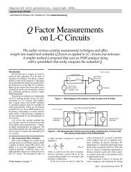
Q <strong>Calculations</strong> <strong>of</strong> L-C<br />
<strong>Circuits</strong> <strong>and</strong> <strong>Transmission</strong><br />
<strong>Lines</strong>: A Unified Approach<br />
Calculate the Q factor <strong>of</strong> any circuit based on its complex<br />
impedance data. These computations allow easy simulation<br />
<strong>and</strong> optimization <strong>of</strong> stub resonators. They apply to RLC circuits,<br />
transmission lines <strong>and</strong> antennas.<br />
Jacques Audet, VE2AZX<br />
Q<br />
factor calculations <strong>of</strong> reactive<br />
circuits are <strong>of</strong> interest since the Q<br />
factor relates directly to the circuit<br />
selectivity: The higher the Q, the better the<br />
selectivity <strong>and</strong> the lower the insertion loss <strong>of</strong><br />
the filter. For oscillators, higher Q also means<br />
that lower phase noise is produced. In the case<br />
<strong>of</strong> antennas, a lower Q is generally preferred,<br />
giving a larger SWR b<strong>and</strong>width.<br />
This paper attempts to clarify the various<br />
methods that can be used to calculate Q factor.<br />
I will show how to calculate the Q factor<br />
using general methods for simple RLC circuit<br />
configurations <strong>and</strong> will show that the<br />
same methods can be used to compute the Q<br />
factor <strong>of</strong> stub resonators <strong>and</strong> antennas operating<br />
outside their resonant frequencies. It<br />
allows computing the SWR b<strong>and</strong>width <strong>of</strong><br />
antennas once the Q factor is known.<br />
The calculations for transmission line<br />
stubs may be carried out using Mathcad files<br />
(described later in the article) with attenuation<br />
data provided by freeware programs<br />
available on the Web. Simulation results will<br />
be presented as well as measured Q values<br />
on a length <strong>of</strong> RG-58 cable.<br />
Simple RX <strong>Circuits</strong><br />
When the internal circuit configuration or<br />
7525 Madrid St<br />
Brossard, QC J4Y 1G3<br />
Canada<br />
ve2azx@amsat.org<br />
Reprinted with permission; copyright ARRL<br />
equivalent circuit is known, we can measure<br />
the complex impedance at a single frequency<br />
<strong>and</strong> calculate the Q <strong>of</strong> that impedance using<br />
the classic relation:<br />
X Rp<br />
Q (Eq 1)<br />
R<br />
s X<br />
where X is the reactance, R s the series resistance<br />
<strong>and</strong> R p the parallel resistance.<br />
The simple series model R s – jX assumes<br />
that the impedance consists <strong>of</strong> a resistance R s<br />
in series with a single reactance X, coming<br />
from a perfect inductance or from a perfect<br />
capacitance. Note that the measurement <strong>of</strong> R s<br />
<strong>and</strong> X only needs to be done at a single frequency.<br />
Examples <strong>of</strong> this are the Q <strong>of</strong> an ideal<br />
inductor or capacitor. In this model, only two<br />
elements are used to describe the impedance.<br />
Since real capacitors all have some series<br />
inductance, we add it in series with the capacitor.<br />
At some frequency the reactances <strong>of</strong> the L<br />
<strong>and</strong> C will cancel <strong>and</strong> the impedance is reduced<br />
to the series R s . Using Equation 1 to compute<br />
the Q factor yields a value <strong>of</strong> zero, since the<br />
total reactance is zero. In general, the above<br />
equation cannot be used to compute the Q factor<br />
when multiple reactances are involved. The<br />
Q factor as obtained from Equation 1 is called<br />
the apparent Q, since it is not generally related<br />
to the resonator selectivity.<br />
In this last case the Q cannot be simply<br />
calculated by Equation 1. The equation does<br />
not tell us the selectivity <strong>of</strong> our circuit since<br />
we now have a resonator. A resonator requires<br />
a minimum <strong>of</strong> two reactive elements that have<br />
opposite signs.<br />
Q Factor <strong>of</strong> Series RLC <strong>Circuits</strong><br />
A simple RLC circuit — series or parallel<br />
— can be used as a resonator. We will<br />
first consider the series RLC configuration.<br />
Here we are interested in the Q factor at resonance<br />
<strong>and</strong> at other frequencies.<br />
The impedance Z <strong>of</strong> the RLC circuit<br />
shows zero reactance at resonance. Then<br />
clearly Equation 1 cannot be used to compute<br />
the Q factor at resonance.<br />
Equation 2 shows how to calculate the Q<br />
factor at resonance <strong>and</strong> below. Note that the<br />
derivative term<br />
dX<br />
dω<br />
implies that the reactance X is effectively calculated<br />
(or measured) at two frequencies: 1, 2<br />
dX<br />
X<br />
<br />
Q<br />
d<br />
a<br />
<br />
(Eq 2)<br />
2 Rs<br />
where<br />
Z Rs<br />
jX,<br />
Rs<br />
Re Z<br />
<br />
<strong>and</strong><br />
X Im Z<br />
1 Notes appear on page 51.<br />
Sep/Oct 2006 43
R s <strong>and</strong> X <strong>and</strong> are the real <strong>and</strong> imaginary components<br />
<strong>of</strong> the RLC circuit impedance Z <strong>and</strong><br />
ω= 2πf.<br />
Equation 2 may be simplified as:<br />
Fr<br />
L<br />
Qa<br />
(Eq 3)<br />
Rs<br />
f C<br />
where Q a is the Q factor below the resonant<br />
frequency F r <strong>and</strong> f is the frequency at which<br />
Q a is calculated.<br />
The resonant frequency may be expressed<br />
as:<br />
1<br />
F r<br />
(Eq 4)<br />
2 LC<br />
After substituting Equation 4 into<br />
Equation 3, we get:<br />
1<br />
Qa<br />
(Eq 5)<br />
2 fCRs<br />
This equation is valid at resonance <strong>and</strong><br />
below.<br />
Equation 5 simply represents the ratio <strong>of</strong><br />
the capacitive reactance to the series<br />
resistance, R s .<br />
An equation similar to Equation 2 may<br />
be used above resonance:<br />
dX<br />
X <br />
Q<br />
d<br />
b<br />
<br />
(Eq 6)<br />
2 Rs<br />
The sign <strong>of</strong> the first term <strong>of</strong> the<br />
numerator, X, is now positive. As before,<br />
Equation 6 may be simplified:<br />
f L<br />
Qb<br />
(Eq 7)<br />
Rs<br />
Fr<br />
C<br />
After substituting Equation 4 into<br />
Equation 7, we get:<br />
2 fL<br />
Q (Eq 8)<br />
Rs<br />
This equation is valid at resonance <strong>and</strong><br />
above.<br />
Equation 8 simply represents the ratio <strong>of</strong><br />
inductive reactance to the series resistance,<br />
R s .<br />
Equations 2 <strong>and</strong> 6 may be combined by<br />
taking the absolute value <strong>of</strong> X in the first<br />
numerator term. Equation 9 gives the Q<br />
factor <strong>of</strong> a series RLC circuit, below <strong>and</strong><br />
above the resonant frequency.<br />
dX<br />
X <br />
Q <br />
d <br />
(Eq 9)<br />
2 R s<br />
This equation is for computing the Q<br />
factor above <strong>and</strong> below series resonance.<br />
Figure 1 shows an example <strong>of</strong> the Q factor<br />
variation versus frequency as computed from<br />
Equation 9 or from Equations 5 <strong>and</strong> 8. Note<br />
that the Q factors calculated by Equations 5<br />
<strong>and</strong> 8 are equal at the resonant frequency <strong>of</strong><br />
10 MHz, since the reactances are also equal.<br />
Above <strong>and</strong> below 10 MHz, the reactances increase,<br />
causing a corresponding increase in the<br />
Q factor. The “<strong>of</strong>f resonance” Q factor gives<br />
the selectivity obtained when a lossless reactance<br />
is used to recover resonance.<br />
Q Factor <strong>of</strong> Parallel RLC <strong>Circuits</strong><br />
The Q factor <strong>of</strong> RLC parallel circuits may<br />
also be calculated with the general formulas<br />
given by Equations 2 <strong>and</strong> 6 above. In this<br />
case, we need to use the admittances instead<br />
<strong>of</strong> the impedances, since the reactance goes<br />
to ±infinity at resonance, with a negative reactance<br />
slope. We then substitute 1/Z for Z<br />
in these equations.<br />
As in series RLC circuits, the Q factor<br />
may also be calculated:<br />
1 d 1 <br />
Im<br />
<br />
Im <br />
Z d Z <br />
Q <br />
1 <br />
2Re<br />
<br />
Z <br />
(Eq 10)<br />
where Re <strong>and</strong> Im are the real <strong>and</strong> imaginary<br />
operators.<br />
This equation is for use below resonance,<br />
after substituting 1/Z for Z in Equation 2.<br />
Equation 10 may be simplified:<br />
R<br />
p<br />
Qa<br />
(Eq 11)<br />
2 fL<br />
This equation is for calculating the Q<br />
below resonance. R p is in parallel with L <strong>and</strong><br />
C.<br />
Above resonance:<br />
1 d 1 <br />
Im <br />
Im <br />
Z d Z <br />
Q <br />
1 <br />
2Re<br />
<br />
Z <br />
(Eq 12)<br />
This equation is for calculating the Q<br />
above resonance.<br />
Equation 12 may be simplified:<br />
Q b = 2 π f C R p (Eq 13)<br />
This equation is for calculating the Q above<br />
resonance.<br />
Equations 10 <strong>and</strong> 12 may be combined<br />
by taking the absolute value <strong>of</strong><br />
1<br />
Im <br />
<br />
<br />
<br />
Z <br />
in the first numerator term. Equation 14 gives<br />
the Q factor <strong>of</strong> a parallel RLC circuit, for<br />
use below <strong>and</strong> above the resonant frequency.<br />
1 d 1 <br />
Im Im <br />
Z d Z <br />
Q <br />
1 (Eq 14)<br />
2Re<br />
<br />
Z <br />
This equation computes the Q factor for<br />
parallel resonance.<br />
<strong>Transmission</strong> Line Stub Resonators<br />
The transmission line stub resonator always<br />
includes three distributed elements: inductance,<br />
capacitance <strong>and</strong> resistance. Taking<br />
a single measurement <strong>of</strong> the complex impedance<br />
at the stub terminals only allows us to<br />
represent the line as a simple two-element<br />
model, with an apparent Q value as given by<br />
Equation 1. It does not allow Q factor predictions<br />
under resonant conditions. While this<br />
is sufficient for some uses, very <strong>of</strong>ten one<br />
needs to know the stub Q factor when the<br />
stub is used as a resonator, with or without a<br />
compensating (loading) reactance. In particular,<br />
it is interesting to know the Q factor <strong>of</strong> a<br />
quarter wavelength resonator, versus one that<br />
is less than a quarter wavelength long <strong>and</strong><br />
brought back to resonance by using capacitive<br />
loading at its open end. In some cases,<br />
the shorter resonator will have a higher Q.<br />
Thus it is useful to know how the resonator<br />
unloaded Q varies versus frequency, length,<br />
Figure 1 — Q factor <strong>of</strong> a<br />
series RLC circuit.<br />
44 Sep/Oct 2006
line attenuation <strong>and</strong> resonator loading such<br />
as capacitive or inductive loads in both open<br />
<strong>and</strong> short configurations.<br />
Estimating the Q factor <strong>of</strong> a “Short”<br />
Unloaded Resonator<br />
In general, Equation 1 above can’t be used<br />
to compute the Q factor for a quarter-wave<br />
resonator, since the reactance value X is zero<br />
or infinite at resonance, <strong>and</strong> will set the Q to<br />
zero or infinity. We also expect a short line<br />
(say 1% <strong>of</strong> wavelength) to behave as lumped<br />
inductance in the case <strong>of</strong> a shorted line <strong>and</strong> a<br />
lumped capacitance in the case <strong>of</strong> an open<br />
line, <strong>and</strong> with a Q factor that can be approximated<br />
by Equation 1.<br />
Computing the Q Factor <strong>of</strong> a Quarter<br />
Wavelength Unloaded Stub, Open or<br />
Shorted — The Easy Way<br />
The simplest way to calculate the Q factor<br />
<strong>of</strong> a quarter wavelength unloaded stub is<br />
to use Equation 15.<br />
8.686 <br />
Q (Eq 15)<br />
Ao<br />
<br />
where A o is the attenuation in dB/100 ft <strong>and</strong><br />
λ is the wavelength in hundreds <strong>of</strong> feet.<br />
Equation 15 may also be written in a more<br />
practical form as:<br />
2.7743 F<br />
Q <br />
o<br />
(Eq 16)<br />
Ao<br />
VF<br />
where F o is the quarter wave resonant frequency<br />
in MHz, A o is the attenuation in dB/<br />
100 ft at F o <strong>and</strong> VF is the velocity factor.<br />
Equation 16 may also be derived from the<br />
attenuation coefficient α <strong>and</strong> the phase coefficient<br />
β: 3<br />
<br />
Q (Eq 17)<br />
2<br />
I have found that Equations 15 to 17 apply<br />
to all unloaded resonators — open or<br />
shorted — whose length is an integer multiple<br />
<strong>of</strong> a quarter wavelength. Note that these<br />
equations do not distinguish between open<br />
<strong>and</strong> shorted quarter wave resonators. It was<br />
found that open <strong>and</strong> shorted resonators have<br />
equal Q factors for a given resonance mode,<br />
no matter their conductor <strong>and</strong> dielectric<br />
losses, as long as we use the same loss values<br />
for both lines.<br />
From Equation 16, given constant values<br />
for A o <strong>and</strong> VF, the Q factor is proportional to<br />
the frequency. In real life, the attenuation<br />
factor A o will increase with frequency, causing<br />
the Q to increase less rapidly.<br />
The line losses, A o , are the total losses.<br />
<strong>Transmission</strong> lines have two loss mechanisms,<br />
however: conductor losses, which are<br />
caused by skin effect, <strong>and</strong> dielectric losses,<br />
which occur in the dielectric material.<br />
In practice, in the HF <strong>and</strong> VHF ranges,<br />
the dielectric losses are much lower than the<br />
conductor losses for coaxial lines. For those<br />
lines, we expect the Q factor <strong>of</strong> opened lines<br />
(subjected to dielectric losses) to be higher<br />
than their shorted equivalent (subjected to<br />
conductor losses) only when their length is<br />
much below a quarter wavelength.<br />
Computing the Q Factor When the Stub<br />
Length is Below or Equal to a Quarter<br />
Wavelength<br />
Computing the Q factor <strong>of</strong> a line requires<br />
knowledge <strong>of</strong> the attenuation due to<br />
conductor losses: A o c in dB/100 feet <strong>and</strong> the<br />
attenuation due to dielectric losses —A o d in<br />
dB/100 ft. The frequency term, f, is in MHz.<br />
A c K f<br />
(Eq 18)<br />
o<br />
1<br />
Ao<br />
d K2<br />
f<br />
(Eq 19)<br />
where K 1 <strong>and</strong> K 2 are respectively the<br />
conductor <strong>and</strong> dielectric losses in dB/100 ft<br />
at 1 MHz.<br />
The K 1 <strong>and</strong> K 2 loss coefficients may be<br />
obtained from the TLDetails.exe program. 4<br />
It gives the coefficients for most coaxial<br />
cables. An accompanying Micros<strong>of</strong>t Excel<br />
file also allows K 1 <strong>and</strong> K 2 calculations for<br />
user-entered attenuation data.<br />
For printed circuit lines such as<br />
microstrips, it is convenient to express the<br />
losses as follows:<br />
Ac<br />
o<br />
f<br />
Acr<br />
o<br />
(Eq 20)<br />
fr<br />
This equation calculates attenuation due<br />
to conductor losses.<br />
f<br />
Ad<br />
o<br />
Adr<br />
o<br />
(Eq 21)<br />
f<br />
r<br />
This equation calculates attenuation due<br />
to dielectric losses.<br />
A Ac Ad<br />
(Eq 22)<br />
o o o<br />
This equation calculates the total losses.<br />
A o is the total attenuation in dB/100 ft,<br />
A o cr is the conductor loss attenuation in dB/<br />
100 ft at frequency f r , f is the frequency, A o dr<br />
is the dielectric loss attenuation in dB/100 ft<br />
at the same frequency, f r .<br />
Note that the conductor losses vary in proportion<br />
to the square root <strong>of</strong> the frequency,<br />
<strong>and</strong> the dielectric losses are proportional to<br />
frequency. The program TXLine.exe may be<br />
used to compute the PCB line attenuations<br />
for various configurations. 5<br />
Note that A o d may also be derived from the<br />
loss tangent, L tan, <strong>of</strong> the dielectric. VF is the<br />
velocity factor <strong>and</strong> f is the frequency in MHz.<br />
efficient, α, <strong>and</strong> the phase coefficient, β:<br />
<br />
<br />
ln 10<br />
A o<br />
(Eq 24)<br />
2000<br />
(Attenuation in neper/foot)<br />
2 f<br />
(Eq 25)<br />
VF ce<br />
(Phase coefficient in radians/foot)<br />
VF is the line velocity factor, c e is the velocity<br />
<strong>of</strong> light in million feet/sec, A o is the<br />
total attenuation in dB/100 ft <strong>and</strong> f is the frequency<br />
in MHz. The complex propagation<br />
coefficient, γ, may now be calculated:<br />
γ = α + jβ (Eq 26)<br />
To properly model the lossy transmission<br />
line, we must compute the complex line impedance,<br />
Z o , using Equation 27. Here the term<br />
R represents the series conductor losses due<br />
to the skin effect <strong>and</strong> dc conductor resistance.<br />
G is a conductance term representing the<br />
parallel dielectric losses. Both R <strong>and</strong> G are a<br />
function <strong>of</strong> the frequency, f, thus making Z o<br />
a complex value, which is also a function <strong>of</strong><br />
the frequency. 6<br />
R<br />
j2<br />
f L<br />
Zo<br />
<br />
6<br />
(Eq 27)<br />
G<br />
j2<br />
f 10 C<br />
In Equation 27, R <strong>and</strong> G are in ohms per<br />
foot <strong>and</strong> siemens per foot, respectively. The<br />
L <strong>and</strong> C are the distributed inductance in μH/<br />
foot <strong>and</strong> capacitance in pF/foot, respectively.<br />
The frequency, f, is in MHz.<br />
The R, L, C <strong>and</strong> G components will be<br />
calculated as follows (See Note 6.):<br />
Im <br />
Z o <br />
L (Eq 28)<br />
2 f<br />
L is in μH per foot.<br />
<br />
Im<br />
Z <br />
o <br />
C <br />
2<br />
f 10<br />
6<br />
(Eq 29)<br />
where C is in pF per foot.<br />
R = 2 α Re[ Z 0 ] (Eq 30)<br />
where R is in ohms per foot.<br />
2 Re<br />
Zo<br />
<br />
G <br />
2<br />
Z<br />
o<br />
(Eq 31)<br />
f<br />
Ad<br />
o<br />
2.78 Ltan<br />
(Eq 23)<br />
VF<br />
We need to compute the attenuation cowhere<br />
G is in siemens per foot<br />
Computing R <strong>and</strong> G requires the knowledge<br />
<strong>of</strong> Z o <strong>and</strong> to compute Z o we need the R<br />
<strong>and</strong> G values. To get around this problem we<br />
use an iterative process where we first use a<br />
real value <strong>of</strong> Z o + j 0 ohms for Z o (the cable<br />
nominal impedance). We then calculate R, L,<br />
G <strong>and</strong> C. These values are then used to recalculate<br />
a new complex value for Z o . This<br />
Sep/Oct 2006 45
Figure 5 — Q factor versus line length for RG-58C, at 16.229 MHz.<br />
Figure 2 — Resonant modes for shorted <strong>and</strong> open lines along<br />
with the relevant equations for Q calculations.<br />
Figure 6 — Q factor versus line length for RG-58C, at 162.29 MHz.<br />
Figure 3 — Q factor <strong>of</strong> a shorted line. Q factor versus frequency for a<br />
10 foot length <strong>of</strong> RG-58C, giving first resonance at ~16.229 MHz (f q<br />
).<br />
Solid line is resonator Q, dotted line is the apparent Q.<br />
Figure 7 — Q factor versus line length at 500 MHz for a 50 Ω<br />
microstrip, 114 mil wide, above a 62 mil thick FR4 substrate.<br />
Figure 4 — Q factor <strong>of</strong> an open line. Q factor versus frequency for<br />
a 10 foot length <strong>of</strong> RG-58C, giving first resonance at ~16.229 MHz<br />
(f q<br />
). Solid line is resonator Q, dotted line is the apparent Q.<br />
process is repeated twice until we get a final value for Z o .<br />
We are now ready to calculate the stub impedances, using the complex<br />
value <strong>of</strong> Z o , for both open <strong>and</strong> short lines. Equation 32 or 33 will<br />
be used to calculate the stub impedances.<br />
Zo<br />
Zsopen<br />
(Eq 32)<br />
tanh( len)<br />
where len is the line length in feet <strong>and</strong> Z o the stub line complex<br />
impedance.<br />
The shorted stub impedance may be calculated as:<br />
46 Sep/Oct 2006
Zsshort Zo<br />
tanh( len)<br />
(Eq 33)<br />
The stub Q factor may now be calculated<br />
as a function <strong>of</strong> frequency or length using<br />
Equation 9 for an open stub, since it behaves<br />
like a series resonant circuit. For a shorted stub,<br />
we use Equation 14 to calculate the Q factor,<br />
just like in the case <strong>of</strong> the RLC parallel circuit.<br />
These calculations are valid below <strong>and</strong><br />
above the quarter wave resonant frequency.<br />
Resonant Modes<br />
Figure 2 shows the resonant modes for<br />
shorted <strong>and</strong> open lines. Equation 14 is used Examples<br />
when the line exhibits parallel resonance <strong>and</strong><br />
Equation 9 when it exhibits series resonance,<br />
just like for discrete RLC resonators. Note that<br />
the shorted line presents an inductive reactance<br />
below the first quarter wave resonance while<br />
the open line is capacitive below resonance.<br />
The Mathcad spreadsheets TRL_Q_Calc1.<br />
mcd for use with the TLDetails.exe program<br />
on coaxial lines <strong>and</strong> TRL_Q_Calc-PCB1.mcd<br />
for use with TXLine.exe program on PCB lines<br />
4, 5, 7<br />
show all above calculations in detail.<br />
<strong>of</strong> Calculated Q factors<br />
versus Frequency for Shorted <strong>and</strong><br />
Opened <strong>Lines</strong> <strong>of</strong> Identical Lengths<br />
Figures 3 <strong>and</strong> 4 show the resonator Q factor<br />
for shorted <strong>and</strong> open lines (a 10-foot length<br />
<strong>of</strong> RG-58C). The solid curves were computed<br />
from Equations 14 <strong>and</strong> 9 as per Figure 2, while<br />
the dotted curves show the ratio <strong>of</strong> reactance<br />
to resistance as computed by Equation 1. This<br />
is the apparent Q. In general, the resonator Q<br />
cannot be computed just by taking the ratio <strong>of</strong><br />
reactance to resistance as in Equation 1. This<br />
Figure 8 — Capacitance in pF required to keep the resonant<br />
frequency at 500 MHz.<br />
Figure 9 — Shorted stub Q factor versus length with the<br />
microstrip resonated with a capacitor having an ESR <strong>of</strong> 0.08 Ω.<br />
Table 1<br />
Mode Freq Shorted Line Open Line Conductor Dielectric<br />
(MHz) EQ. Used Calc Q Q error EQ. Used Calc Q Q error Losses Losses<br />
dB/100 ft dB/100 ft<br />
1X 10 14 28
approximation is valid for frequencies below<br />
25% <strong>of</strong> the quarter wave resonant frequency<br />
(~16.229 MHz), however. For both shorted <strong>and</strong><br />
open stubs, Equation 16 may be used to calculate<br />
the Q factor at all integer multiples <strong>of</strong> a<br />
quarter wavelength.<br />
Using a constant real value for the line<br />
impedance makes the Q factor versus frequency<br />
equal for both open <strong>and</strong> shorted lines.<br />
This method makes calculations much faster<br />
<strong>and</strong> simpler, but as shown in Figures 3 <strong>and</strong> 4,<br />
it will give very large errors in the Q <strong>and</strong> in<br />
the complex stub impedance. I also discovered<br />
that the common transmission line models<br />
used in my pr<strong>of</strong>essional RF-microwave<br />
circuit simulator use this shortcut too.<br />
Note the Q factor behavior below the quarter<br />
wave frequency F q . At frequencies below<br />
F q , the Q factor goes down for the shorted<br />
line while it goes up for the open line. This<br />
tells us that the line losses are mostly in the<br />
conductors (~1.8 dB/100 ft while the dielectric<br />
losses are ~ 0.14 dB/100 ft. at the quarter<br />
wave resonant frequency).<br />
It is also interesting to compute the Q factor<br />
versus line length at a fixed frequency.<br />
Figure 5 shows the Q factor at 16.229 MHz<br />
for a 10-foot length <strong>of</strong> RG-58C cable. Again<br />
the open line has a much higher Q factor below<br />
the quarter wave resonant length <strong>of</strong> 10 feet.<br />
Figure 6 shows the Q factor versus line<br />
length for a 1 foot length <strong>of</strong> RG-58C line.<br />
Decreasing the line length by a factor <strong>of</strong> 10<br />
has increased its resonant frequency by the<br />
same factor <strong>and</strong> the Q at self resonance goes<br />
from 36 to 100, a factor <strong>of</strong> ~3. This is possible<br />
since the losses are mainly conductor<br />
losses: 5.77 dB/100 ft <strong>and</strong> the dielectric losses<br />
are 1.36 dB/100 ft at 162.29 MHz. Note also<br />
that the loss tangent <strong>of</strong> the dielectric is 0.002.<br />
In contrast, PCB losses will be much<br />
higher with say, FR4 which has a typical loss<br />
tangent <strong>of</strong> 0.02<br />
The Q factor for a 50-Ω microstrip<br />
trace has been computed in Figure 7. The<br />
PCB loss tangent is 0.02 <strong>and</strong> the trace<br />
length is 3.469 inches to obtain quarter<br />
wave resonance at 500 MHz. At that frequency,<br />
the conductor losses are 5.7 dB/<br />
100 feet <strong>and</strong> the dielectric losses are<br />
47.5 dB/100 feet.<br />
Note that the open line now has its Q factor<br />
almost constant below quarter wave resonance.<br />
The Q factor <strong>of</strong> the shorted line is now<br />
much higher, in fact the shorter the line the<br />
higher the Q. The shorted stub becomes attractive<br />
as a resonator by using shorter lines<br />
with the higher Q. Then a low loss capacitor<br />
will be required to bring the line back to resonance<br />
at 500 MHz.<br />
Figure 8 shows the required stub loading<br />
capacitance versus line length to resonate at<br />
500 MHz. When the line length approaches<br />
a quarter wavelength, the required loading<br />
capacitance decreases toward zero.<br />
Real capacitors have a series resistance<br />
that limits their Q factor, however. In<br />
the next example, a series resistance <strong>of</strong><br />
0.08 Ω is assumed. The effective Q factor<br />
<strong>of</strong> the stub <strong>and</strong> the capacitor may be computed<br />
by recalling that the Q factors add<br />
like parallel resistors. There is now an<br />
optimum length that will provide the highest<br />
Q, which is around 1 inch or about<br />
25% <strong>of</strong> the original self resonant length.<br />
See Figure 9.<br />
The highest Q will generally be obtained<br />
by paralleling multiple capacitors<br />
to decrease the effective series resistance.<br />
Note that wider PCB traces will provide<br />
higher Q factors, even if the line Z o is<br />
lower.<br />
Substituting RG-174 coax gives a<br />
maximum Q <strong>of</strong> 100 at 2.5 inches, while a<br />
length <strong>of</strong> RG-213 shows a maximum Q <strong>of</strong><br />
394 at a quarter wavelength (3.9 inches).<br />
This means that a low to very-low-loss line<br />
will have its highest Q at a quarter wavelength<br />
<strong>and</strong> above. I have measured the<br />
unloaded Q <strong>of</strong> a 6-inch-diameter quarterwave<br />
resonator at 145 MHz in quarterwave<br />
mode <strong>and</strong> 430 MHz in ¾-wave mode.<br />
At 145 MHz, the unloaded Q was 5324<br />
<strong>and</strong> 9065 at 430 MHz: an increase by a<br />
factor <strong>of</strong> 1.7. This is also predicted by the<br />
models presented here.<br />
Note that adding a lossless reactance<br />
in parallel (or series) with the stub — to<br />
modify its resonant frequency — does not<br />
change its Q versus frequency as calculated<br />
from Equations 9 or 14. Only its resonant<br />
frequency is changed.<br />
So far from these simulations, Equations<br />
9 <strong>and</strong> 14 make sense for calculating<br />
the resonator unloaded Q for resonator<br />
lengths ranging from 1% <strong>of</strong> the wavelength<br />
to many wavelengths. At low frequencies<br />
where the resonator is less than 1 /16 wavelength,<br />
we get the same results by simply<br />
taking the reactance-to-resistance ratio to<br />
compute the Q factor instead <strong>of</strong> using the<br />
more complex Equations 9 <strong>and</strong> 14.<br />
Validating the Computed Resonator Q<br />
from the Calculated Stub Impedance<br />
A second method <strong>of</strong> calculating the<br />
resonator Q factor has been used to determine<br />
the limits <strong>of</strong> validity <strong>of</strong> Equations 9<br />
<strong>and</strong> 14 as applied to transmission lines.<br />
The resonator Q may be determined by<br />
finding the two frequencies f 1 <strong>and</strong> f 2 around<br />
the stub resonance that yield a stub impedance<br />
with a phase angle <strong>of</strong> ±45°. The<br />
exact stub resonant frequency is f r , where<br />
its input reactance is zero in the case <strong>of</strong><br />
series resonant lines. For lines that are<br />
parallel resonant, we use admittances <strong>and</strong><br />
note the frequency where the suceptance<br />
goes to zero. For Q factors above 10, f r<br />
can be taken as the average <strong>of</strong> f 1 <strong>and</strong> f 2 .<br />
The stub Q factor can then be calculated<br />
from:<br />
f r<br />
Q <br />
(Eq 34)<br />
f<br />
2<br />
f<br />
1<br />
Note that the stub impedance measurements<br />
may be done at either end <strong>of</strong> the line,<br />
without affecting the Q value.<br />
This method may also be used to compute<br />
the Q factor at frequencies other than at<br />
resonance by adding a lossless frequencydependant<br />
series reactance (L or C) in the<br />
case <strong>of</strong> a series resonant line. Similarly, parallel<br />
resonant lines require the addition <strong>of</strong> a<br />
susceptance in shunt with the line. This<br />
method was used to verify the accuracy <strong>of</strong><br />
Equations 9 <strong>and</strong> 14 with the help <strong>of</strong> Mathcad<br />
to do the calculations.<br />
Table 1 summarizes the results for a line<br />
length <strong>of</strong> 8.17 feet. The frequency for the<br />
losses is 5 MHz. The Q error was derived by<br />
using Equation 34 to compute the resonator<br />
Q from the impedance/admittance data <strong>and</strong><br />
comparing the values obtained with Equations<br />
9 or 14.<br />
At 28 MHz, we are about halfway between<br />
resonances, <strong>and</strong> either Equations 9 or<br />
14 may be used, for both shorted <strong>and</strong> opened<br />
lines. This value is the geometric average<br />
between the first <strong>and</strong> second resonances.<br />
As it can be seen from Table 1, the error<br />
is largest for Q values below 20 or so. The<br />
worst errors occur at the highest resonance<br />
modes having the lowest Qs. Below quarter<br />
wave resonance, the Q error is below 1% for<br />
Qs above 10.<br />
Computing Resonator Q from B<strong>and</strong>width<br />
Measurements at Multiples <strong>of</strong><br />
Quarter Wavelength Resonance<br />
Another way to verify the resonator Q<br />
factor is to build a b<strong>and</strong>-pass filter <strong>and</strong> measure<br />
its selectivity by measuring its –3 dB<br />
points on an S21 display. To precisely determine<br />
the resonator Q u (unloaded Q), the coupling<br />
<strong>of</strong> the stub under test to the source <strong>and</strong><br />
detector will have to be very small. Equation<br />
34 is used to compute the resonator Q factor.<br />
Figure 10 shows the circuit that I have used<br />
for my simulations on a line, which behaves<br />
as a parallel LC resonator.<br />
In Figure 10, the source <strong>and</strong> detectors have<br />
low impedance (50 Ω). The stub is coupled<br />
to the source-detector via 0.1 pF capacitors.<br />
This method is useful to determine the resonant<br />
frequency <strong>of</strong> a shorted quarter wave line,<br />
since it presents the highest impedance at<br />
resonance. Again, Equation 34 is used to<br />
compute the stub unloaded Q factor, where<br />
f 1 <strong>and</strong> f 2 are the –3 dB frequencies, as measured<br />
from the resonant frequency f r . Note<br />
that the source <strong>and</strong> load resistive impedances<br />
will decrease the Q factor somewhat. Equation<br />
35 may be used to calculate the unloaded<br />
48 Sep/Oct 2006
Q, based on the measured attenuation at the<br />
resonant frequency <strong>and</strong> percent b<strong>and</strong>width.<br />
Computing Resonator Q from B<strong>and</strong>width<br />
Measurements below Quarter<br />
Wavelength Resonance<br />
Figure 11 shows the setup that may be<br />
used with series resonant RLC elements<br />
when the resonant line is inductive or capacitive.<br />
The total reactance is cancelled, leaving<br />
the series R s at resonance. This series R s<br />
is easily determined by doing an attenuation<br />
test (S21) in a 50-to-50 Ω circuit at the series<br />
resonant frequency. The equivalent L <strong>and</strong><br />
C lumped elements must also be determined<br />
by doing two more attenuation tests, before<br />
one can calculate the Q factor. I have developed<br />
an Excel file that does these calculations:<br />
Calc_SeriesRLC.xls. 7 Note that the C<br />
element has to be replaced by an inductor<br />
when the stub impedance is capacitive.<br />
Tests were done on a 100-inch length <strong>of</strong><br />
RG-58 cable, by measuring the complex reflection<br />
coefficient over 201 frequency<br />
points, using a lab-quality vector <strong>net</strong>work<br />
analyzer (HP 8753D). See Figure 12. The<br />
measured coefficients were then converted<br />
to impedance data using Mathcad. The Q<br />
factor was calculated as per Equations 9 <strong>and</strong><br />
14 (solid curves) <strong>and</strong> as per Equation 1 (dotted<br />
curves). These dotted curves show the<br />
cable resonant frequencies; for example,<br />
where the reactance is zero: 19.4 MHz <strong>and</strong><br />
38.8 MHz.<br />
Figure 10 — Measuring <strong>and</strong> computing<br />
resonator Q from b<strong>and</strong>width measurements.<br />
Shorted <strong>and</strong> Open Line Measurements<br />
In Figure 12, the shorted line exhibits parallel<br />
resonance at 19.4 MHz, <strong>and</strong> Equation<br />
14 is used to compute the resonator Q factor<br />
up to 27 MHz. Equation 9 is used from<br />
27 MHz up to 50 MHz, since we have a series<br />
resonance at 38.8 MHz.<br />
For the open line <strong>of</strong> Figure 13, the equations<br />
are used in the reverse order. Note that<br />
the open line has a higher Q factor. The above<br />
Q curves are representative <strong>of</strong> a line that has<br />
much less dielectric losses than conductor<br />
losses as in Figures 3 <strong>and</strong> 4. Note the Q curve<br />
sloping down below 3 MHz. This is possibly<br />
caused by the inaccuracies in the measurements,<br />
especially for resistive impedance<br />
values below 5 Ω.<br />
Measured Q Values versus Computed<br />
Values<br />
Table 2 shows the percentage error between<br />
measured Q factors versus the computed values<br />
at three frequencies. Notice that there is<br />
good agreement between the two. The measured<br />
Q was computed directly from attenuation<br />
measurements, as per Figures 10 <strong>and</strong> 11.<br />
A series inductor was used to resonate the line<br />
when its reactance is capacitive <strong>and</strong> vice-versa.<br />
The Q <strong>of</strong> the inductor was measured <strong>and</strong> its<br />
series resistance was subtracted from the total<br />
series resistance to obtain the actual stub series<br />
resistance. This data was then used to correct<br />
the resistive part <strong>of</strong> the VNA measurements,<br />
by calculating the <strong>of</strong>fset between the<br />
two measurements. This correction is only<br />
valid around the test frequency. Then the Q<br />
was computed using the corrected VNA measurements,<br />
with Equations 9 <strong>and</strong> 14.<br />
Table 3 shows the calculated <strong>and</strong> measured<br />
Q factors at the (approximate) quarter<br />
wave frequency. The calculated values were<br />
obtained from the Equations 14 <strong>and</strong> 9, while<br />
the measured values were done by impedance<br />
measurements, using Equation 34. Keep<br />
in mind that the measured Q value for open<br />
line has probably more errors, since the resistive<br />
part <strong>of</strong> the impedance is around 1 Ω.<br />
The conductor losses are dominant here<br />
<strong>and</strong> we can also use equation 16 to compute<br />
the resonator Q based on the measured stub<br />
attenuation in dB/100 ft. The Q value obtained<br />
is 32.00 at 19.375 MHz.<br />
Using the Resonator as a B<strong>and</strong>pass<br />
Filter<br />
Knowing the unloaded Q, as calculated<br />
Figure 12 — Measured Q<br />
factor <strong>of</strong> a shorted line.<br />
Computed Q factor<br />
versus frequency (solid<br />
lines, from impedance<br />
measurements) for a<br />
100 inch length <strong>of</strong> RG-58,<br />
giving first resonance at<br />
~19.4 MHz. Compare<br />
these to simulations in<br />
Figures 3 <strong>and</strong> 4. The<br />
dotted lines show the<br />
apparent Q.<br />
Table 2<br />
Shorted Line<br />
Open Line<br />
Frequency (MHz) % Q error Frequency (MHz) % Q error<br />
Figure 11 — Measuring <strong>and</strong> computing<br />
resonator Q below quarter wavelength<br />
resonance.<br />
9.33 2.7 4.92 2.9<br />
28.93 2.1 28.93 1.5<br />
Table 3<br />
Shorted Line<br />
Open Line<br />
Frequency (MHz) Calculated Q (Eq 14) Measured Q Frequency (MHz) Calculated Q (Eq 9) Measured Q<br />
19.375 35.3 19.375 36.36<br />
19.106 34.43 19.334 30.95<br />
Sep/Oct 2006 49
above, allows us to compute the insertion loss<br />
<strong>of</strong> a single resonator b<strong>and</strong>pass filter based<br />
on the percent b<strong>and</strong>width.<br />
100 <br />
Loss 20 log 1 (Eq 35)<br />
<br />
KQ <br />
u <br />
Equation 35 shows the relation between<br />
the unloaded Q (Q u ), K the percentage b<strong>and</strong>width<br />
(ratio <strong>of</strong> b<strong>and</strong>width to center frequency<br />
in %) <strong>and</strong> the resonator losses in dB. 8 For<br />
instance, a 2% b<strong>and</strong>width with a Q u <strong>of</strong> 200<br />
will give an insertion loss <strong>of</strong> 2.5 dB.<br />
Q Factor <strong>of</strong> Antennas<br />
Equations 9 (for open circuit antennas) <strong>and</strong><br />
14 (for closed loop antennas) may also be used<br />
to calculate the Q factor <strong>of</strong> antennas, based on<br />
their impedance data. I have provided a<br />
Mathcad file that does impedance calculations<br />
on a monopole for various lengths. 7, 9 The<br />
monopole is treated as a transmission line<br />
whose average impedance Z a is given by:<br />
Z a = 60 ln (hd) (Eq 36)<br />
where hd is the length-to-radius ratio. Here,<br />
the radiation resistance is proportional to the<br />
frequency to the power 1.7. It is added to the<br />
conductor losses.<br />
Figure 14 gives the simulated monopole<br />
Q factor. Once the Q factor is known, the<br />
b<strong>and</strong>width, BW, may be easily calculated<br />
using Equation 37. The b<strong>and</strong>width obtained<br />
gives the frequencies where the impedance<br />
phase angle is ±45°.<br />
BW<br />
f<br />
r<br />
(Eq 37)<br />
Q<br />
where f r is the center frequency.<br />
This b<strong>and</strong>width, as calculated from the Q<br />
factor, corresponds to the 7 dB return loss<br />
points or to an SWR <strong>of</strong> ~2.62. For a 2:1 SWR,<br />
the b<strong>and</strong>width is 70% <strong>of</strong> the above. This assumes<br />
that the SWR is 1:1 at resonance.<br />
Conclusion<br />
In this paper I have shown that a single<br />
general equation may be used to calculate<br />
the Q factor <strong>of</strong> RLC circuits <strong>and</strong> transmission<br />
lines as it relates to circuit selectivity. I<br />
have shown that series resonances are taken<br />
care by Equation 9 while Equation 14 takes<br />
care <strong>of</strong> parallel resonances. The difference<br />
between the two is the use <strong>of</strong> impedances for<br />
the first <strong>and</strong> admittances for the second equation.<br />
By using the provided Mathcad files <strong>and</strong><br />
the associated public domain programs, it is<br />
easy to compute the Q factor <strong>of</strong> coaxial <strong>and</strong><br />
microstrip or stripline resonators for any<br />
length <strong>and</strong> frequency. The calculated Q factor<br />
agrees very well with the measured data<br />
<strong>and</strong> with the Q values computed by the impedance<br />
measurement method. When simulating<br />
stub resonators, it is very important that<br />
the full R L G C transmission line models be<br />
used. The Mathcad files show how to optimize<br />
the Q factor <strong>of</strong> PCB microstrip <strong>and</strong><br />
stripline resonators. The same files also show<br />
the calculations <strong>of</strong> R L C G functions <strong>and</strong><br />
coefficients to be incorporated into any RF<br />
simulation s<strong>of</strong>tware. It is interesting to note<br />
that these four frequency dependent parameters<br />
fully describe the transmission line. I<br />
found that the Q values predicted from Equations<br />
9 <strong>and</strong> 14 fully agree with the values<br />
obtained in the simulation s<strong>of</strong>tware.<br />
The simulations presented here show that it is<br />
possible to get higher Q factors on low-loss lines<br />
by using higher-order modes, such as ¾ λ. For<br />
PCB resonator traces, the optimum Q is generally<br />
below a quarter wavelength.<br />
Note that the models presented here do<br />
not take into account the radiation losses <strong>and</strong><br />
surface roughness <strong>of</strong> microstrips. The line dc<br />
resistance has been included in the PCB line<br />
models, since its contribution is not negligible<br />
at narrow trace widths. For coaxial<br />
lines, the dc resistance has been omitted to<br />
keep the models simpler <strong>and</strong> relieve the user<br />
from searching for the resistance data. This<br />
makes the coaxial models less accurate below<br />
approximately 5 MHz. The dc resistance<br />
may be added to the ac conductor resistance<br />
by taking the square root <strong>of</strong> the sum <strong>of</strong> the<br />
squares <strong>of</strong> the dc <strong>and</strong> ac resistances, as done<br />
in the file: TRL_Q_Calc-PCB1.mcd.<br />
Thanks to Chase Hearn <strong>and</strong> Yan Gunmar<br />
for triggering this study <strong>and</strong> providing<br />
various helpful references <strong>and</strong> comments.<br />
Appendix<br />
An intuitive view <strong>of</strong> the general function<br />
for calculating the Q factor is derived here.<br />
The general equation for computing the<br />
Q factor <strong>of</strong> RLC circuits, transmission line<br />
resonators <strong>and</strong> antennas operating in the series<br />
resonant mode is given by the source at<br />
Note 1. This equation is valid from low frequencies,<br />
though series resonance <strong>and</strong> for<br />
frequencies much above series resonance.<br />
X<br />
Q <br />
<br />
dX<br />
<br />
<br />
<br />
2 R d<br />
<br />
(Eq A1)<br />
<br />
Where ω = 2π f, the radian frequency, R<br />
<strong>and</strong> X are respectively the real <strong>and</strong> imaginary<br />
parts <strong>of</strong> the impedance .<br />
Equation A1 may be written in terms <strong>of</strong><br />
the frequency:<br />
f <br />
dX X <br />
Q <br />
<br />
2 R df f <br />
<br />
(Eq A2)<br />
Figure 13 — Measured Q factor <strong>of</strong> an open line. Computed Q<br />
factor versus frequency (solid lines, from impedance<br />
measurements) for a 100 inch length <strong>of</strong> RG-58, giving first<br />
resonance at ~19.4 MHz. Compare these to simulations in Figures<br />
3 <strong>and</strong> 4. The dotted lines show the apparent Q.<br />
Figure 14 — Monopole Q factor (solid curve) as calculated from<br />
the Mathcad file: Monopole-Ralph.mcd. The quarter wave<br />
resonance is at 6 MHz, as shown by the dotted line curve<br />
(apparent Q) which was calculated from the reactance to<br />
resistance ratio. Note the steep increase in Q as the frequency is<br />
lowered. This comes from the fact that the radiation resistance<br />
decreases approximately as frequency to the power 1.7. At 1 MHz<br />
<strong>and</strong> below we have a low-loss air insulated capacitor!<br />
50 Sep/Oct 2006
Notice that the first term <strong>of</strong> Equation A2<br />
represents the Q factor at resonance, when X<br />
= 0.<br />
f <br />
Q<br />
dX <br />
<br />
2 R <br />
df<br />
<br />
(Eq A3)<br />
<br />
This equation gives the Q Factor at resonance,<br />
as very <strong>of</strong>ten seen in textbooks.<br />
Applying Equation A2 for a series resonant<br />
circuit, for frequencies well above the<br />
resonant frequency, we get:<br />
dX <br />
2 L<br />
df<br />
<br />
(Eq A4)<br />
<br />
Recall that the reactive component comes<br />
from the inductance.<br />
f 2<br />
fL <br />
Qhf<br />
<br />
2<br />
L<br />
2 R f (Eq A5)<br />
<br />
<br />
where Q hf is the Q factor for frequencies well<br />
above the resonant frequency. This simplifies<br />
to:<br />
2 fL XL<br />
Qhf<br />
(Eq A6)<br />
R R<br />
where X L is the inductive reactance. This is<br />
the same as Equation 1 in the main text —<br />
valid well above the resonant frequency.<br />
For frequencies well below the resonant<br />
frequency, where the reactance component<br />
comes from the capacitance, we get:<br />
dX <br />
<br />
<br />
Q<br />
1<br />
df 2<br />
2 f C<br />
lf<br />
f <br />
<br />
2 R <br />
<br />
<br />
1 1 <br />
<br />
f C f C f <br />
2<br />
2 2<br />
(Eq A7)<br />
<br />
(Eq A8)<br />
Q lf is the Q factor for frequencies well<br />
below the resonant frequency.<br />
After simplification:<br />
1 X<br />
C<br />
Qlf<br />
(Eq A9)<br />
2 fRC R<br />
where X C is the capacitive reactance — valid<br />
well below the resonant frequency. This is<br />
the same as Equation 1 in the main text.<br />
Notes<br />
1 Peter Vizmuller, RF Design Guide, Artech<br />
House, Norwood, MA, 1995, p. 235.<br />
2 The Small Koch Fractal Monopole: Theory, design<br />
<strong>and</strong> applications, p 6. See www-personal.engin.<br />
umich.edu/~lschulwi/koch.pdf<br />
3 Pr<strong>of</strong>essor Niknejad, Lectures on Lossy <strong>Transmission</strong><br />
<strong>Lines</strong> <strong>and</strong> the Smith Chart, University<br />
<strong>of</strong> California, Berkeley. Course EECS 117, Lecture<br />
6: www-inst.eecs. berkeley.edu/~ee117/<br />
sp04/lect/lecture6.pdf<br />
4 The program TLDetails.exe may be downloaded<br />
from Dan Maguire, AC6LA. Download<br />
from www.ac6la.com/tldetails.html<br />
e-mail: ac6la@arrl.<strong>net</strong><br />
5 The program TXLine.exe may be downloaded<br />
from www.mw<strong>of</strong>fice.com/prod-<br />
ucts/txline.html (you will need to register.)<br />
6 Frank Witt, AI1H, “<strong>Transmission</strong> Line Properties<br />
from Manufacturer’s Data,” ARRL<br />
Antenna Compendium Vol. 6, ARRL,<br />
1999, pp 179 - 183 <strong>and</strong> related Mathcad<br />
files on the accompanying CD-ROM.<br />
7 The Mathcad files TRL_Q_Calc1.mcd <strong>and</strong><br />
TRL_Q_Calc-PCB1, Monopole-Ralph.mcd<br />
<strong>and</strong> the Excel file: Calc_SeriesRLC.xls may<br />
be downloaded from the ARRL Web at<br />
www.arrl.org/qexfiles/. Look for 9x06_<br />
Audet.zip.<br />
8 R<strong>and</strong>all W. Rhea, HF Filter Design <strong>and</strong><br />
Computer Simulation, section 5.5, Noble<br />
Publishing.<br />
9 Ralph Holl<strong>and</strong>, “Impedance <strong>of</strong> Wide Regular<br />
Structures,” antennex.com/archive3/<br />
archive3.htm. You must be an antenneX<br />
subscriber to view this article.<br />
Jacques Audet, VE2AZX, became interested<br />
in radio at the age <strong>of</strong> 14, after playing with<br />
crystal radio sets <strong>and</strong> repairing old receivers.<br />
At 17, he obtained his first ham license. In 1967<br />
he obtained his B Sc degree in electrical engineering<br />
from Laval University. He then worked<br />
in engineering functions at Nortel Networks,<br />
where he retired in 2000. He worked mostly in<br />
test engineering on a number <strong>of</strong> products <strong>and</strong><br />
components operating from dc to light-wave<br />
frequencies. His areas <strong>of</strong> interest are in RF<br />
simulations, filters, duplexers, antennas <strong>and</strong><br />
using computers to develop new test techniques<br />
in measurement <strong>and</strong> data processing.<br />
Introducing the... AntennaSmith tm !<br />
Patent Pending<br />
TZ-900 Antenna Impedance Analyzer<br />
2 Sec Sweeps, Sweep Memories, 1 Hz steps, Manual &<br />
Computer Control w/s<strong>of</strong>tware, USB, low power. Rugged<br />
Extruded Aluminum Housing - Take it up the tower!<br />
■ Full Color TFT LCD Graphic Display<br />
■ Visible in Full Sunlight<br />
■ 0.2 - 55 MHz<br />
■ SWR<br />
NEW!<br />
■ Impedance (Z)<br />
■ Reactance (r+jx)<br />
Now Shipping!<br />
■ Reflection coefficient (ρ,θ<br />
ρ,θ)<br />
■ Smith Chart<br />
Check Your Antennas <strong>and</strong> Transmisson <strong>Lines</strong><br />
Once you use the TZ-900 -<br />
you’ll never want to use any other!<br />
651-489-5080 Fax 651-489-5066<br />
sales@timewave.com www.timewave.com<br />
1025 Selby Ave., Suite 101 St. Paul, MN 55104 USA<br />
Check Our<br />
New Line-up:<br />
HamLinkUSB tm Rig Control<br />
TTL Serial Interface with PTT<br />
HamLinkBT tm Remote Control<br />
U232 tm RS-232-to-USB Universal<br />
Conversion Module replaces<br />
PCB-mount DB-9 & DB-25<br />
PK-232 /USB Multimode Data<br />
Controller (upgrades available)<br />
PK-96/USB TNC (upgrades available)<br />
Timewave - The Leader in<br />
Noise & QRM Control:<br />
DSP-599zx Audio Signal<br />
Processor<br />
ANC-4 Antenna Noise Canceller<br />
From the Timewave<br />
Fountain <strong>of</strong> Youth -<br />
Upgrades for many <strong>of</strong> our DSP &<br />
PK products!<br />
Sep/Oct 2006 51