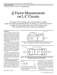
Q Calculations of L-C Circuits and Transmission Lines ... - Ve2azx.net

above, allows us to compute the insertion loss
of a single resonator bandpass filter based
on the percent bandwidth.
100
Loss 20 log 1 (Eq 35)
KQ
u
Equation 35 shows the relation between
the unloaded Q (Q u ), K the percentage bandwidth
(ratio of bandwidth to center frequency
in %) and the resonator losses in dB. 8 For
instance, a 2% bandwidth with a Q u of 200
will give an insertion loss of 2.5 dB.
Q Factor of Antennas
Equations 9 (for open circuit antennas) and
14 (for closed loop antennas) may also be used
to calculate the Q factor of antennas, based on
their impedance data. I have provided a
Mathcad file that does impedance calculations
on a monopole for various lengths. 7, 9 The
monopole is treated as a transmission line
whose average impedance Z a is given by:
Z a = 60 ln (hd) (Eq 36)
where hd is the length-to-radius ratio. Here,
the radiation resistance is proportional to the
frequency to the power 1.7. It is added to the
conductor losses.
Figure 14 gives the simulated monopole
Q factor. Once the Q factor is known, the
bandwidth, BW, may be easily calculated
using Equation 37. The bandwidth obtained
gives the frequencies where the impedance
phase angle is ±45°.
BW
f
r
(Eq 37)
Q
where f r is the center frequency.
This bandwidth, as calculated from the Q
factor, corresponds to the 7 dB return loss
points or to an SWR of ~2.62. For a 2:1 SWR,
the bandwidth is 70% of the above. This assumes
that the SWR is 1:1 at resonance.
Conclusion
In this paper I have shown that a single
general equation may be used to calculate
the Q factor of RLC circuits and transmission
lines as it relates to circuit selectivity. I
have shown that series resonances are taken
care by Equation 9 while Equation 14 takes
care of parallel resonances. The difference
between the two is the use of impedances for
the first and admittances for the second equation.
By using the provided Mathcad files and
the associated public domain programs, it is
easy to compute the Q factor of coaxial and
microstrip or stripline resonators for any
length and frequency. The calculated Q factor
agrees very well with the measured data
and with the Q values computed by the impedance
measurement method. When simulating
stub resonators, it is very important that
the full R L G C transmission line models be
used. The Mathcad files show how to optimize
the Q factor of PCB microstrip and
stripline resonators. The same files also show
the calculations of R L C G functions and
coefficients to be incorporated into any RF
simulation software. It is interesting to note
that these four frequency dependent parameters
fully describe the transmission line. I
found that the Q values predicted from Equations
9 and 14 fully agree with the values
obtained in the simulation software.
The simulations presented here show that it is
possible to get higher Q factors on low-loss lines
by using higher-order modes, such as ¾ λ. For
PCB resonator traces, the optimum Q is generally
below a quarter wavelength.
Note that the models presented here do
not take into account the radiation losses and
surface roughness of microstrips. The line dc
resistance has been included in the PCB line
models, since its contribution is not negligible
at narrow trace widths. For coaxial
lines, the dc resistance has been omitted to
keep the models simpler and relieve the user
from searching for the resistance data. This
makes the coaxial models less accurate below
approximately 5 MHz. The dc resistance
may be added to the ac conductor resistance
by taking the square root of the sum of the
squares of the dc and ac resistances, as done
in the file: TRL_Q_Calc-PCB1.mcd.
Thanks to Chase Hearn and Yan Gunmar
for triggering this study and providing
various helpful references and comments.
Appendix
An intuitive view of the general function
for calculating the Q factor is derived here.
The general equation for computing the
Q factor of RLC circuits, transmission line
resonators and antennas operating in the series
resonant mode is given by the source at
Note 1. This equation is valid from low frequencies,
though series resonance and for
frequencies much above series resonance.
X
Q
dX
2 R d
(Eq A1)
Where ω = 2π f, the radian frequency, R
and X are respectively the real and imaginary
parts of the impedance .
Equation A1 may be written in terms of
the frequency:
f
dX X
Q
2 R df f
(Eq A2)
Figure 13 — Measured Q factor of an open line. Computed Q
factor versus frequency (solid lines, from impedance
measurements) for a 100 inch length of RG-58, giving first
resonance at ~19.4 MHz. Compare these to simulations in Figures
3 and 4. The dotted lines show the apparent Q.
Figure 14 — Monopole Q factor (solid curve) as calculated from
the Mathcad file: Monopole-Ralph.mcd. The quarter wave
resonance is at 6 MHz, as shown by the dotted line curve
(apparent Q) which was calculated from the reactance to
resistance ratio. Note the steep increase in Q as the frequency is
lowered. This comes from the fact that the radiation resistance
decreases approximately as frequency to the power 1.7. At 1 MHz
and below we have a low-loss air insulated capacitor!
50 Sep/Oct 2006