Plenoptic Principal Planes - Todor Georgiev

Plenoptic Principal Planes
Todor Georgiev Andrew Lumsdaine Sergio Goma
Adobe Systems, Inc. Indiana University Qualcomm
tgeorgie@adobe.com lums@cs.indiana.edu sgoma@qualcomm.com
Abstract: We show that the plenoptic camera is optically equivalent to an array of cameras.
We compute the parameters that establish that equivalence and show where the plenoptic
camera is more useful than the camera array.
© 2011 Optical Society of America
OCIS codes: 000.0000, 999.9999.
1. Introduction
In 1908, Lippmann introduced the idea of using a microlens array to capture the radiance of a scene and produce what
he called integral photographs [1]. These photographs displayed not just a 2D picture, but also “the 3D relief” of the
scene [2]. In 1928, Ives subsequently added an objective lens to Lippmann’s microlens array [3] to increase the acuity.
Since then, many other researchers and scientists have continued to advance integral photography.
With the advent of digital photography, significant new opportunities to investigate integral photography became
available. In 1992, Adelson introduced the “plenoptic camera,” a digital version of Lippmann’s microlens array designed
to solve problems in computer vision [4]. In 2005, Ng improved the plenoptic camera and introduced new
digital-processing methods, including refocusing [5, 6]. In later work Fife [7] and Lumsdaine and Georgiev [8] improved
the resolution by introducing the focused plenoptic camera and developed methods for rendering synthetic
views with computational focus at high resolution.
In parallel with this, researchers have also used arrays of ordinary cameras to capture multiple views, reconstruct
the plenoptic function, and render synthetic refocused views [9]. Designs using a single camera, but with arrays of
lenses in front of the main lens have also been proposed [10].
Thus, we have two families of systems for capturing the plenoptic function: those with a single main lens and
a microlens array and those with multiple cameras (multiple main lenses). A natural question then arises regarding
these two families. Are these two families equivalent in some sense or are they fundamentally different? In this paper
we prove that these two families are in fact optically equivalent and we derive the parameters that establish this
correspondence.
2. Principal Planes in Integral Photography
In ray optics light transport is described by the ray matrices of the corresponding optical elements [11]. These matrices
act on the ray vector (q, p), where q is the displacement away from the optical axis, p is the slope. Since in Gaussian
optics the system is linear, the joint action of all elements is described by the product of their matrices in the order in
which light encounters them when travelling through an optical system.
A lens of focal length f and a translation of distance t are respectively described by the ray matrices
L( f ) =
[ 1 0
− 1 f
1
]
, T (t) =
[
1 t
0 1
]
. (1)
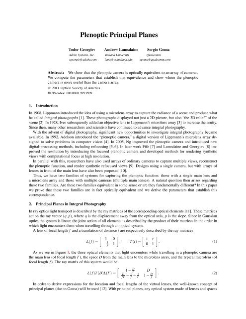
As we see in Figure 1, the three optical elements that light encounters while travelling in a plenoptic camera are
the main lens (of focal length F), the space D from the main lens to the microlens array, and the typical microlens (of
focal length f ). The ray matrix of this system would be
[
L( f )T (D)L(F) =
1 − D F
D
D
f F − 1 f − F
1 1 − D f
]
. (2)
In order to derive expressions for the location and focal lengths of the virtual lenses, the well-known concept of
principal planes (due to Gauss) will be used [12]. With principal planes, any optical system made of lenses and spaces

etween them can be replaced with an optically equivalent system consisting of space from the entrance to the “first
principal plane”; followed by refraction by appropriate lens; followed by travel from a “second principal plane” to the
exit. Mathematically, this means that the matrix corresponding to any optical system can be formed as the product of
three matrices:
[
1 y
T (y)L(Φ)T (x) =
0 1
][ 1 0
− 1 Φ 1 ][
1 x
0 1
] [ 1 −
y
= Φ
− 1 Φ
x + y − xy
Φ
1 −
Φ
x
]
. (3)
Note that the distances x and y don’t have to add up to the total distance travelled, and the principal planes may actually
be outside the system (in this case x and/or y are negative).
Now we equate the system matrix described by (2) with the principal
planes system matrix (3). By making the bottom left matrix element in (2)
and (3) equal, we derive the focal length Φ of the effective lens. Similarly
we derive the distances x and y.
Fig. 1: The concept of principal planes
applied to the plenoptic camera. Only
one microlens is shown.
Φ =
F f
F + f − D , x = DF
f + F − D , y = D f
f + F − D . (4)
For the incoming light the virtual lens is positioned at the first principal
plane; for the sensor the virtual lens is positioned at the second principal
plane. It is well known that the focused plenoptic camera exists in two versions:
As an array of Keplerian or Galilean telescopes. Distances and focal
lengths are positive or negative depending on which type of focused plenoptic
camera we are using, with real or virtual image of the main lens image.
3. Cameras
A typical focused plenoptic camera is described in Lumsdaine and
Georgiev [8]. We will establish the exact equivalence of this camera with an
appropriate camera array. The main lens has focal length F = 140mm. All microlenses have focal length f = 750µm.
We consider the two types of camera separately.
3.1. Keplerian case
The value of D can be freely modified by the user in such a way that the denominator F + f − D actually goes through
zero. To get a reasonable value of D, let’s assume that the world is at infinity, and that the main lens image is formed
at a distance of 6 f in front of the microlens. Such settings are typical for a real camera. Then a simple calculation
shows that the focal length Φ = −28mm, and the distances are x = −5226mm, and y = −28mm, approximately.
Figure 2 shows the dependence of the focal length of the virtual lens on the value of D. The two branches of the graph
correspond to the Keplerian and Galilean cases. The specific value of Φ = −28mm is represented as a dot.
Fig. 2: Focal length of the virtual lens
as a function of the distance D between
main lens and microlens.
We see that the equivalent virtual lens is negative, i.e. the image is not
flipped. That’s what we actually observe in the captured imagery: Microimages
are not flipped relative to the world. Flipping two times in the relay
system is equal to no flip. More interesting, the virtual lens is placed at big
negative x, far in front of the camera. This is as if the plenoptic camera has
an array of negative lenses in front, very similar to the camera described
in [10]. The distance y is also negative. That’s natural considering that the
image of a negative lens is actually formed in front of it. It is also as expected
that the image of an object at infinity is formed at one focal length
from the lens.
The distance between microlenses is d = 250µm. Considering similar
triangles in the camera geometry, the distance between the virtual lenses that
are in front of the main lens would be xd/D = 9.3mm. Again, we observe
approximately same size as that of the negative lenses that were placed in
front of the camera in the case of [10].

3.2. Galilean case
To fix the value of D let’s assume that the world is at infinity, and the main lens image is formed at a distance of
6 f behind the microlens. Then a simple calculation shows that the focal length Φ = 28mm, and the distances are
x = 5226mm, and y = 28mm, approximately. We see that the virtual lens is positive and the image would be flipped.
That’s what we actually observe in the captured imagery. The virtual lens is placed at big positive x, far behind the
camera (as in a Galilean telescope). The distance y is also positive. It is as expected that the image of an object at
infinity is formed at one focal length behind the lens.
In both the Keplerian and Galilean cases the difference from a camera array is that now the lenses are virtual, and
we can acually position them within a big range, inclucing locations that are mechanically not accessable. Also, our
equations are very sensitive to the value of the denominator F + f − D so we can easily tune and vary the distances
within a wide range, including infinity.
4. Conclusion
In this paper we have presented a proof that the two approaches to radiance capture, the plenoptic and the multicamera
array, are equivalent. We establish the correspondence between the plenoptic camera and the array of cameras based
on the concept of principal planes, and we compute the parameters for that correspondence in two typical cses.
In our opinion the two main factors that make the plenoptic camera preferable to the camera array are the smaller
size, and the lower cost of a quality plenoptic implementation – compared to the corresponding equivalent camera
array. Also, the great flexibility in the positioning the virtual lenses in the plenoptic camera can be practically useful.
References
1. G. Lippmann, “Épreuves réversibles. Photographies intégrales,” Académie des sciences pp. 446–451 (1908).
2. G. Lippmann, “Epreuves reversibles donnant la sensation du relief,” Journal of Physics 7, 821–825 (1908).
3. H. E. Ives, “A camera for making parallax panoramagrams,” Journal of the Optical Society of America 17,
435–439 (1928).
4. E. Adelson and J. Wang, “Single lens stereo with a plenoptic camera,” IEEE Transactions on Pattern Analysis
and Machine Intelligence pp. 99–106 (1992).
5. R. Ng, M. Levoy, M. Bredif, G. Duval, M. Horowitz et al., “Light field photography with a hand-held plenoptic
camera,” Tech. Rep. 2005-02, Stanford University Computer Science (2005).
6. R. Ng, “Digital light field photography,” Ph.D. thesis, Stanford University, Stanford, CA, USA (2006). Adviser-
Patrick Hanrahan.
7. K. Fife, A. E. Gamal, and H.-S. P. Wong, “A 3Mpixel multi-aperture image sensor with 0.7µm pixels in 0.11µm
CMOS,” in “IEEE ISSCC Digest of Technical Papers,” (IEEE, 2008), pp. 48–49.
8. A. Lumsdaine and T. Georgiev, “The focused plenoptic camera,” in “IEEE International Conference on Computational
Photography (ICCP),” (IEEE, 2009).
9. M. Levoy and P. Hanrahan, “Light field rendering,” Proceedings of the 23rd annual conference on Computer
Graphics and Interactive Techniques (1996).
10. T. Georgiev, K. Zheng, B. Curless, D. Salesin, and et al., “Spatio-angular resolution tradeoff in integral photography,”
Proc. Eurographics Symposium on Rendering (2006).
11. A. Gerrard and J. M. Burch, Introduction to Matrix Methods in Optics (Dover Publications, 1994).
12. T.-G. Fischer, Optical System Design (PIE Press, 2000).