Covariant Derivatives and Vision - Todor Georgiev

Covariant Derivatives and Vision
Todor Georgiev
Adobe Systems, 345 Park Ave, W10-124, San Jose, CA 95110, USA
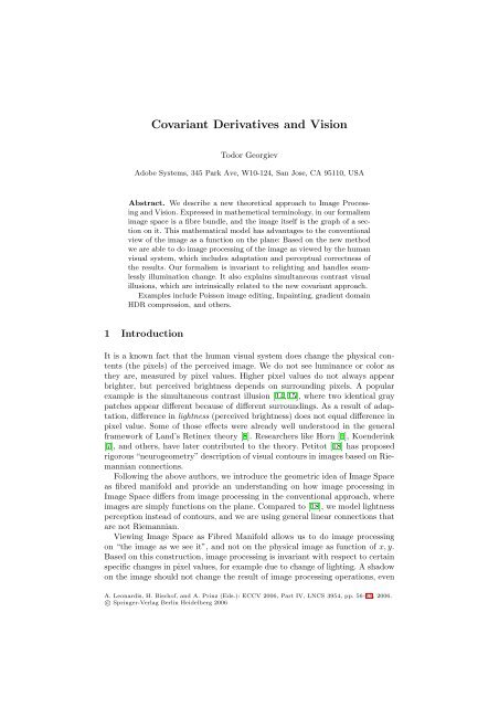
Abstract. We describe a new theoretical approach to Image Processing
and Vision. Expressed in mathemetical terminology, in our formalism
image space is a fibre bundle, and the image itself is the graph of a section
on it. This mathematical model has advantages to the conventional
view of the image as a function on the plane: Based on the new method
we are able to do image processing of the image as viewed by the human
visual system, which includes adaptation and perceptual correctness of
the results. Our formalism is invariant to relighting and handles seamlessly
illumination change. It also explains simultaneous contrast visual
illusions, which are intrinsically related to the new covariant approach.
Examples include Poisson image editing, Inpainting, gradient domain
HDR compression, and others.
1 Introduction
It is a known fact that the human visual system does change the physical contents
(the pixels) of the perceived image. We do not see luminance or color as
they are, measured by pixel values. Higher pixel values do not always appear
brighter, but perceived brightness depends on surrounding pixels. A popular
example is the simultaneous contrast illusion [14, 15], where two identical gray
patches appear different because of different surroundings. As a result of adaptation,
difference in lightness (perceived brightness) does not equal difference in
pixel value. Some of those effects were already well understood in the general
framework of Land’s Retinex theory [8]. Researchers like Horn [6], Koenderink
[7], and others, have later contributed to the theory. Petitot [18] has proposed
rigorous “neurogeometry” description of visual contours in images based on Riemannian
connections.
Following the above authors, we introduce the geometric idea of Image Space
as fibred manifold and provide an understanding on how image processing in
Image Space differs from image processing in the conventional approach, where
images are simply functions on the plane. Compared to [18], we model lightness
perception instead of contours, and we are using general linear connections that
are not Riemannian.
Viewing Image Space as Fibred Manifold allows us to do image processing
on “the image as we see it”, and not on the physical image as function of x, y.
Based on this construction, image processing is invariant with respect to certain
specific changes in pixel values, for example due to change of lighting. A shadow
on the image should not change the result of image processing operations, even
A. Leonardis, H. Bischof, and A. Prinz (Eds.): ECCV 2006, Part IV, LNCS 3954, pp. 56–69, 2006.
c○ Springer-Verlag Berlin Heidelberg 2006

Covariant Derivatives and Vision 57
if it changes pixel values. A good edge detection (or face detection) system is
not influenced by change of lighting.
We discuss in detail one example of how this new approach works: Writing
the Laplace equation in terms of connections automatically improves the results
of Poisson image editing [10]. Other examples include Inpainting [2], Gradient
domain high dynamic range compression [5], and the Bilateral filter [13], [4].
2 Image Space as Fibred Manifold
2.1 Motivation
Intuitively, our approach can be described as follows. A grayscale image is not
a collection of pixels, but a collection of “fibres”. Instead of each pixel having
brightness, we have “a mark” on each fibre. The bundle of fibres is “dynamic” in
the sense that we can freely “slide” fibres relative to one-another. This happens
as part of the Retinex-type adaptation of our visual system. Even though the
mark on the fibre (pixel value) remains the same, its relation to the other fibres
is different. This creates the preception of lightness as different from luminance.
On a more rigorous level, we propose to use the mathematical concept of
Fibre Bundle [12], [9]. It assumes no a priori relation among fibres, other than
topological. The relation (comparison between fibres) is added later, when we
introduce a connection. It gives meaning to pixels by making comparison of
lightness possible.
The relation among pixels is to some extent ’added’ by the observer and is
due to both pixel value and adaptation of the visual system. If captured in
appropriate mathematical formalism, this will influence image processing.
The ultimate goal is to be able to do image processing on the internal image
that we see, while actually touching only the physical pixels.
2.2 Image Space
In the traditional approach grayscale images are represented as surfaces in R 3 :
Pixels are defined by their coordinates x, y in the image plane, and their corresponding
values z in R + . Thus, the conventional model of image space is
Cartesian product of the image plane and the positive real line of pixel values,
R 2 ×R + . This structure contains two natural projections: For any point in image
space we can immediately say which pixel it is, and what the pixel value is –
according to the two components of the Cartesian product. In this model the
image is a function z = f(x, y), and there is a natural comparison between any
two pixel values: simply z2 − z1. It is customary to assume that brightness of
different pixels can be compared in this way.
However, as noticed in section 2.1, there are examples of same pixel values
appearing different or difference in lightness not equal to difference in pixel value.
Retinex and other adaptation theories are fundamentally based on considering
this difference between pixel values and lightness.

58 T. Georgiev
The fact that the human visual system does not compare pixels by their luminance
alone, suggests that we need a model of image space in which pixel values,
even if well defined, are not comparable a priori. It should be possible to add
comparison or “difference in observed lightness” later, after a given adaptation.
We propose a model that replaces the Cartesian product structure of Image
Space with a Fibred Space structure (see also [7]). The new structure is “weaker”
because it “forgets” (in the mathematical sense) one of the projections (on z).
In this paper we will show on several examples how this fibred space structure
can be useful. Intuitively, the new structure is essentially a Cartesian product
with one of the projections relaxed. By having the freedom of introducing this
projection later (based on the concept of connection) we gain control on effects
of adaptation.
This situation is similar to the model of space-time in classical mechanics [9].
There is a natural projection on time, in the sense that all observers have one
absolute time. For example, they can synchronize their watches.
However, there is no natural projection onto space. One observer thinks that
a given object does not move: It is always “here”, in the sense that projection
onto space is giving the same location at any time. However, another observer
who passes by in a car would see that this same object moving. It projects onto
different locations in space throughout time. Projection onto space is different
for different observers!
In this way, space-time in classical mechanics is not simply a Cartesian product
of space and time. Space in mechanics is relative, it depends on how we define
the second projection. Time is absolute. Space acts like our “fibres” in images
- it depends on the frame of reference or, which is the same, on the observer.
Current pixel values are simply one possible set of coordinates for the image, like
the coordinates of objects relative to one particular observer (in a given moving
car). Other pixel values may describe the same mental image.
To continue the analogy, velocity in mechanics is like perceived gradients in
images. It is different from the point of view of different observers, just like
perceived image gradient depends on the state of adaptation of the observer.
2.3 Fibred Space
By definition [12], a Fibred Space (E, π, B) consists of two spaces: total space
E and base space B, and a mapping π, called projection, of the total space onto
the base. Space B has lower dimension than E, somanyE points map to the
same B point, as shown in Figure 1.
In our model of grayscale images the total space is R 3 , the base is the image
plane, and π gives us the location of each pixel in the image plane. There is no
mapping that would give us the grayscale value of lightness for a pixel.
For each point p ∈ B there is the so-called fibre (Fp in Figure 2) in E, consisting
of all points that are sent to p by π (definition of fibre). We cannot compare
the lightness of two points from different fibres because in the mathematical
structure there is no mapping that would produce that lightness. Each fibre has
its luminance coordinate, but luminances in different fibres are not related.

Fig. 1. Fibred space (E, π, B)
Covariant Derivatives and Vision 59
By definition, a section in a Fibred Space is a mapping f that sends points
in B to E, and has the property π(f(p)) = p for any p ∈ B. See Figure 2.
Fig. 2. Section in fibred space (E, π, B)
A section selects just one of the many points in each fibre. It defines one
manifold (connected set of points) in total space E, with one point in E for each
point in B. Intuitively it is “the closest we can get to the concept of function
without defining a function”.
A grayscale image is a section in a fibred image space (R 3 , π, R 2 ). Since there
is no projection onto z, there is no comparison between different pixels. As a
result, change in image lightness and directional derivative at a point in image
space is not defined. Pixels are simply records and come without interpretation.
Luminance or pixel value is a perceptually meaningless coordinate.
2.4 Connections
In fibred spaces changes in the section (slopes of the section) are measured by
the so called connection, orcovariant derivative (instead of derivative). As the
name suggests, connections show how fibres are “connected” or “glued together”.
Connections are used like derivatives to compare pixel values from different fibres.
In Physics [3] the simplest example of such a field is the vector potential
in Electrodynamics.
In order to introduce the definition of connection in a natural way, let us first
consider the gradient when the image is defined traditionally as a function f(x, y)
on the image plane. The gradient is a vector ( ∂f ∂f
∂x , ∂y ) with two components that
are functions of x, y.

60 T. Georgiev
If the image is defined as a section in a fibred space, the above definition of
gradient does not work because in fibred spaces there is no concept of derivative
or “comparison between different fibres”. Perceptually the situation is similar.
We do not have a sense of comparison between the lightness of different pixels in
the image before assuming some adaptation of the visual system. Pixels are just
“records” without interpretation. In order to compare pixels we need an additional
structure. In our mathematical model this structure is called connection.
A connection on a bundle (E,π,B), where B denotes the image plane, is a
mapping, or a rule, that for any section σ on E produces what is called the x and
y components of the covariant gradient of that section. These components are
also sections. This mapping has certain properties similar to the properties of
the gradient. In order to come up with a natural definition, let’s look again at the
case of functions. If f = f(x, y) ands = s(x, y) are functions on B, the derivative
of the product fs in direction x would be ∂
∂
∂
∂x (fs)=( ∂xf)s + f ∂xs,whichis known as the Leibniz rule for derivative of a product. A similar expression is
valid for the y derivative.
The concept of connection is a generalization of the above Leibniz rule to the
case of sections. By definition, if D is a connection, Dx(fσ)=( ∂
∂xf)σ + fDxσ.
Note that the derivative ∂ acts on a function, while the “derivative” acting on
∂x
the section is Dx. Similar expression is valid for y.
In our image processing applications, a color picture is a section in a vector
bundle, where each three dimensional fibre is a copy of the vector space of
colors. A connection is “adapted (covariant) gradient of color”, as perceived by
the observer. In other words, it shows how the human visual system in a given
state of adaptation perceives directional change of color.
Any section can be represented as a linear combination of a set of basis sections
σi. Inotherwords,σ = Σfiσi. Summation is assumed over i =1, 2, 3, and the
coefficients f i are functions. These functions are referred to as color channels
(Photoshop terminology).
By the above definition of connection, Dx and Dy would act on a section
σ = Σfiσi in the following way:
Dxσ = DxΣ(f i σi) =Σ(( ∂
∂x f i )σi + f i Dxσi) (1)
Dyσ = DyΣ(f i σi) =Σ(( ∂
∂y f i )σi + f i Dyσi) (2)
These expressions simply extend the Leibniz rule for the action of derivatives
on functions to a Leibniz rule for sections. We don’t know what the action on
the basis section σi is, but we know that the result must be again a section,
representable by the basis. So, it is Dxσi = ΣAj ixσj where Aj ix is some matrixvalued
function of x and y. Similar for Dy and Aj iy.
DxΣ(f i σi) =Σ(( ∂
∂x f i )σi + Σf i A j ixσj) (3)
DyΣ(f i σi) =Σ(( ∂
∂y f i )σi + Σf i A j iyσj) (4)

Covariant Derivatives and Vision 61
As a matter of notation, often the basis σi is dropped, and we talk of the
section as represented in terms of f i . Then the action of the connection on fi is:
Dxf i = ∂
∂x f i + ΣA i j xf j . (5)
Dyf i = ∂
∂y f i + ΣA i j yf j . (6)
This expression for the connection, as a replacement of the derivative, will
be our main tool throughout this paper. The rule of thumb is that a connection
Dx, Dy replaces the gradient ∂ ∂
∂x , ∂y according to the so called “minimal
substitution”:
∂
∂x → Dx = ∂
∂x + Ax. (7)
∂
∂y → Dy = ∂
∂y + Ay. (8)
The expression ∂
∂x + Ax and similar for y is called the covariant derivative, or
perceptual gradient.
In color images Ax and Ay are matrix valued functions of x, y. Ingrayscale
images Ax and Ay are functions.
Summary of the result to this point: In fibred spaces changes in the section are
measured by a connection, instead of derivative. As the name indicates, connections
show how we compare, or transfer pixel values from one fibre to another, in
other words - how fibres are “connected”. In Physics [3], connections are called
covariant derivatives. A classical example of connection is the Electromagnetic
field, represented by the vector potential A.
We would like to end this section with a perceptual example of how connections
work in images. The image is a section in a fibre bundle, where we have no
a priori comparison between pixel values in different fibres. As such, the image
is a record without any interpretation. Adaptation, expressed as a connection, is
what gives meaning to pixels, making comparisons possible in terms of lightness.
To make this all more intuitive, let’s look at the example. The simultaneous
contrast illusion, Figure 3 shows that humans do not perceive pixel values directly.
(See [14, 15] for a general survey on lightness perception and examples of
illusions.) In the figure there is a constant gray band surrounded by a variable
background. Due to our visual system’s adaptation, the band appears to vary in
lightness in opposition to its surroundings. Pixel gradient is zero, but perceived
or covariant gradient is not zero. The reason why we see change of lightness
in the constant band is the nonzero covariant derivative by which we compare
pixels.
Next we will be working with grayscale images, assuming the generalization
to three color channels is straight forward.
2.5 Covariantly Constant Sections
Following formulas (7) and (8), we will be representing any section by the corresponding
function, replacing gradients with covariant gradients. Since now we

62 T. Georgiev
Fig. 3. The central rectangle has constant pixel values
have a way to compare pixels and calculate derivatives, we can ask the question:
When is a given section constant?
Any section g(x, y) can be considered constant relative to appropriately chosen
adaptation Ax,Ay, such that ( ∂
∂x + Ax)g = 0, and similar for y. The solution is:
Ax = − 1 ∂g
(9)
g ∂x
Ay = − 1 ∂g
(10)
g ∂y
We are considering Retinex-type adaptation of the visual system, in which the
perceived gradient is the covariant derivative. In grayscale images it is described
by a vector field Ax,Ay). When the visual system is exactly adapted to the
image in a given area, so that (9) and (10) are satisfied, we see constant gray
image (or image matching the surrounding color). We call this state complete
adaptation to the image. In practice, due to the unconscious motion of the eyes, a
state of complete adaptation is very difficult to reach. Still, the idea of complete
adaptation will be very useful in the following sections.
3 Test Case 1: Poisson Image Editing
3.1 Equations
It is well known that the Laplace equation △f = 0 with Dirichlet boundary
conditions is the simplest way to reconstruct (or inpaint) a defective area in an
image. It can be used to remove scratches, wrinkles, or bigger unwanted objects.
Let’s write the derivatives in the Laplacian △ explicitly:
∂ ∂ ∂ ∂
f + f =0, (11)
∂x ∂x ∂y ∂y
After performing the minimal substitution (7), (8), the Laplace equation (11) is
converted into the covariant Laplace equation:
( ∂ ∂
+ Ax)(
∂x ∂x + Ax)f +( ∂ ∂
+ Ay)(
∂y ∂y + Ay)f =0, (12)

which after performing the differentiation can be written as
Covariant Derivatives and Vision 63
△f + fdivA +2A · gradf + A · Af =0. (13)
Here the vector function A(x, y) =(Ax(x, y),Ay(x, y)) describes adaptation of
the visual system, and f(x, y) is the function that represents the grayscale image
as a section. The minimal substitution above is equivalent to the transition from
the conventional image model as a function to the new model of the image as a
section on a fibre bundle. The Laplace equation is converted into the covariant
Laplace equation, which is in fact closer to Poisson equation.
Next we assume A represents complete adaptation to a selected area where
the image is a section defined by g(x, y), translated. The solution of (13) would
be smooth if observed with eyes adapted to g(x, y), but the solution will look
like having g(x, y) “imprinted on it” if observed in some other more typical state
of adaptation. Since state of complete adaptation is practically never achieved,
solving (13) is a way of reconstructing some area with texture similar to g. At
the same time this reconstruction is exact as a model of how the adapted visual
system would “solve” the Laplace equation to fill in the selected region.
Notice that now A(x, y) =− gradg
g can be interpreted as playing the role of
the “guidance field” in Poisson image editing [10]. Substituting in equation (13),
we obtain the final form of the covariant Laplace equation:
△f
f
− 2 gradf
f
· gradg
g
− △g
g
Let’s compare it with the Poisson equation used in [10]:
+2(gradg) · (gradg)
g 2 =0. (14)
△f = △g (15)
We see that the covariant Laplace equation is more complicated than (15). It
can be viewed as a Poisson equation with a modified △g term on the “right hand
side”. The structure of the equation prescribed by our model is very specific. It
prescribes the expression 2gradf · gradg △g (gradg)·(gradg)
g + f g − 2f g2 as the correct
one to choose as a source term in the modified Poisson equation for seamless
cloning. Equation (15) can be viewed as a simplified approximation.
3.2 Results
One of the practical results of this paper is that the new covariant equation
(14) produces seamless cloning of better quality compared to Poisson editing.
By simple differentiation we can see that (14) is equivalent to:
△ f
= 0 (16)
g
Equation (16) is easy to solve in 3 steps:
(1) Divide the image f by the texture image g, in which pixel value zero
is replaced with a small number. This produces the first intermediate image
I1(x, y).

64 T. Georgiev
f(x, y)
I1(x, y) =
g(x, y)
(2) Solve the Laplace equation for the second intermediate image
(17)
△I2(x, y) =0, (18)
with Dirichlet boundary conditions defined by I1(x, y) at the boundary of the
reconstruction area.
(3) Multiply the result by the texture image g(x, y)
h(x, y) =I2(x, y)g(x, y), (19)
and substitute the original defective image f(x, y) with the new image h(x, y)
in the area of reconstruction.
A multigrid approach to solving (18) with good performance is described in
[11]. In practical terms, the tool works sufficiently fast for using it in interactive
mode. For example, on a laptop running Windows XP with a 2 GHz Pentium 4
processor, applying a brush of radius 100 pixels takes less than 0.25 seconds to
converge.
We apply the algorithm to fix a scratch in Figure 4. Figure 5 shows a zoom
in, where the areas to clone from and to clone into are indicated.
Figure 6 (left) shows the result of Poisson Cloning by solving (15), and comparison
with Covariant cloning based on the proposed method (right). The example
was not selected in any special way. We see that the result is slightly better in
terms of matching the contrast. This behavior is repeated consistently in other
experiments, especially in areas of changing shadows/illumination. Sometimes
the difference between the two methods is big, sometimes - small, but the covariant
approach is always better.
Another example is taken from [16]. The authors use a version of Poisson
cloning to fuse night and day images so that in a day image we can see clear
Fig. 4. Basilica San Marco, Venice

Fig. 5. Areas and direction of cloning
Covariant Derivatives and Vision 65
Fig. 6. Poisson cloning (left) and Covariant cloning (right)
Fig. 7. Two methods of cloning from the night scene
representation of the night version of the same scene. In Figure 7 the right side
of each image has been modified by cloning from the night image. We see that
Poisson cloning looks blurry, while Covariant cloning looks better.

66 T. Georgiev
4 Test Case 2: Image Inpainting
The method of Inpainting [2] works similar to solving the Laplace equation
to reconstruct the selected area based on the boundaries. However, based on a
higher order PDE related to fluid dynamics the method is able to partially reconstruct
“structure” inside the inpainted area by continuation of the surrounding
grayscale values into the inside. The behavior often resembles fluid flow and
sometimes is not exactly what we want. Later research attempts to also reconstruct
the texture which is extracted from the surroundings using mathematical
results from functional analysis [17].
Figure 8 compares Inpainting (left) with “Structure and texture” Inpainting
[17] (middle) and our new method of Covariant Inpainting. We would like to
thank G. Sapiro and K. Patwardhan for producing the first two pictures. Our
method is equivalent to replacing the derivatives in conventional Inpainting with
covariant derivatives. As in the previous test case, the result is achieved in three
steps. (1) Divide the original image by the texture image. (2) Solve the PDE, in
this case the Inpainting PDE in the selected region. (3) Multiply by the texture
image. We see that our result is better than both previous methods.
Fig. 8. From left to right: Inpainting, Structure and texture inpainting, Covariant
inpainting
5 Test Case 3: Gradient Domain High Dynamic Range
Compression
This section will be a theoretical derivation of previous results. As in previous
sections, the value is in the new theoretical understanding and in showing that
our approach has a wide area of applicability. We will be looking at the invariance
properties of our fibre bundle approach in the case of relighting and adaptation
to the new illumination of the scene.
A central problem in dealing with high dynamic range images (HDR) is how
to display them on a low dynamic range device, like a monitor. Just like scratch
removal, the problem of HDR compression can be expressed in terms of relighting.
As an example of how our method works, we will reproduce the results of
one of the best approaches [5] starting from first principles.

Covariant Derivatives and Vision 67
Here is a short review of the algorithm of [5]: Treat only the luminance, f.
Calculate logarithm F =lnf; find the gradient of it; attenuate big gradients to
reduce dynamic range; then integrate back to get a real image in log space; and
finally take the exponent to produce the output luminance.
The logarithm of luminance is used simply because human visual system is
approximately logarithmic, and not based on theoretical reasons. Our approach
will provide theoretical justification of the use of logarithm.
The authors minimize the following energy written in log-space
�
( ∂
∂x F − Ax) 2 +( ∂
∂y F − Ay) 2 dxdy (20)
to produce the Poisson equation
△F = divA (21)
for the logarthm of luminance, where A is the attenuated gradient of the log of
the input. “Integrate back” in the above algorithm means “solve (21)”. Without
attenuation, (21) would produce seamless cloning from any image g if A = gradg
g .
We can also write G =lng and then
△F = △G. (22)
Now, let’s do the same with our approach. The energy expression is written
based on requirements for adaptation invariance. In other words, a multiplicative
shadow/relighting g on the source image produces an additive to Aµ term in such
a way that the new output image is multiplied by the same shadow/relighting.
This simple requirement for energy invariance produces the result (21), (22),
automatically placed in log-space. The transforms are:
f → gf (23)
A → A − gradg
. (24)
g
The simplest energy expression that has the above invariance can easily be written
using covariant derivatives:
� ∂ (( ∂x + Ax)f) 2 +(( ∂
2
∂y + Ay)f)
f 2 dxdy. (25)
If we substitute A with − gradg
g , the Euler-Lagrange equation for this energy
would be:
△ ln f = △ ln g, (26)
which is exactly (22). In this way, we have found an invariant under (23), (24)
energy expression that reproduces the results of [5].
Because of the logarithm in our result, we reproduce exactly (22), the same as
[5]. What is the difference in our approach? We did not depend on intuition to

68 T. Georgiev
motivate this use of log space; instead, it comes directly from our mathematical
model based on first principles. This can be seen as theoretical motivation for
using log space in any visual system.
Note that A is adaptation vector field, and it can be more general than gradient
of a function. We adapt to what we see, and not to the pixel values of
energy illuminating the retina. Due to these adaptation effects, what we see is
not always representable in pixels or as a picture. In other words, the human
visual system can produce internally things that can not possibly be represented
as a picture (on a monitor or other device).
6 Other Test Cases and Future Research
As future research we are looking into more rigorous application of our approach
to color images, which are naturally represented as sections in vector bundles.
For example, the above Gradient Domain High Dynamic Range Compression [5]
has been applied only on a grayscale image (or the luminance channel), and it
would be useful to see what modifications could we bring with the fibre bundle
approach.
Another test case would be the Bilateral [13] and Trilateral [4] filters, which are
treating Image Space in the spirit of Bundles, filtering both in ’Domain’ (image
plane) direction and in ’Range’ (pixel value) direction. This type of filtering can
be captured in the mathematical formalism of Jet Bundles [12].
But the main idea of our current paper was that we need to use expressions
for the energy based on connections (covariant derivatives) acting on images
as sections, not functions. This could be done in relation to any PDE or other
image processing algorithm, not just the Laplace equation and Inpainting, and
this defines a wide area of research.
References
1. Adobe Systems: Photoshop 7.0 User Guide. Adobe Systems, San Jose, 2002.
2. M. Bertalmio, G. Sapiro, V. Castelles, C. Ballester, ”Image Inpainting,” Proceedings
of ACM SIGGRAPH 2000, pp. 417-424, ACM Press, 2000.
3. Y. Choquet-Bruhat, C. DeWitt-Morette, Analysis, Manifolds and Physics, Amsterdam,
North-Holland, 1982.
4. P. Choudhury, J. Tumblin, ”The Trilateral Filter for High Contrast Images and
Meshes,” Proceedings of the 2003 Eurographics Symposium on Rendering, pp.186-
196, 2003.
5. R. Fattal, D. Lischinski, M. Werman, ”Gradient Domain High Dynamic Range
Compression,” Proceedings of ACM SIGGRAPH 2002, pp. 249-256, 2002.
6. B. Horn, ”Determining Lightness from an Image,” Computer Graphics and Image
Processing, 3, pp. 277-299, 1974.
7. J. Koenderink, A. van Doorn, ”Image Processing Done Right,” Proceedings of
ECCV 2002, pp. 158-172, Springer, 2002.
8. E. Land, J. McCann, ”Lightness and Retinex Theory,” Journal of the Optical
Society of America, v. 61, no. 1, pp. 1-11, 1971.

Covariant Derivatives and Vision 69
9. L. Mangiarotti, G. Sardanashvily, Gauge Mechanics, World Scientific, North-
Holland, 1998.
10. P. Prez, M. Gangnet, A. Blake, ”Poisson Image Editing,” Proceedings of ACM
SIGGRAPH 2003, pp. 313-318, 2003.
11. W. Press, S. Teukolsky, W. Vetterling, B. Flannery, Numerical Recipes in C, Cambridge
University Press, 1992.
12. D. Saunders, The Geometry of Jet Bundles, Cambridge University Press, 1989.
13. C. Tomasi, R. Manduchi, ”Bilateral Filtering for Gray and Color Images.” Proceedings
IEEE Int. Conf. on Computer Vision, pp. 836-846, 1998.
14. M. Gazzaniga, The New Cognitive Neurosciences, MIT Press, Cambridge, MA,
2000, pp. 339-351.
15. A. Seckel, The Art of Optical Illusions, Carlton Books, 2000.
16. R. Raskar, A. Ilie, J. Yu, “Image Fusion for Enhancing Context in Images and
Video.” ACM Nonphotorealistic Animation and Rendering (NPAR) 2004.
17. M. Bertalmio, L. Vese, G. Sapiro, S. Osher, “Simultaneous Structure and Texture
Image Inpainting.” CVPR (2) 2003, pp. 707-712
18. J. Petitot, “The neurogeometry of pinwheels as a sub-Riemannian contact structure.”
Journal of Physiology - Paris 97, 2003, pp. 265-309.