Dynamic Performance of a SCARA Robot Manipulator With ...
Dynamic Performance of a SCARA Robot Manipulator With ...
Dynamic Performance of a SCARA Robot Manipulator With ...

You also want an ePaper? Increase the reach of your titles
YUMPU automatically turns print PDFs into web optimized ePapers that Google loves.
IEEE TRANSACTIONS ON ROBOTICS, VOL. 25, NO. 1, FEBRUARY 2009 207<br />
TABLE I<br />
<strong>SCARA</strong> PARAMETERS FOR NUMERICAL STUDY<br />
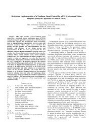
Fig. 1. Schematic <strong>of</strong> the <strong>SCARA</strong> robot showing the geometric parameters and<br />
coordinate frames.<br />
where M is the mass matrix, C is a vector <strong>of</strong> Coriolis and centrifugal<br />
terms, G is the gravitational terms, and τ is a vector <strong>of</strong> generalized<br />
forces. These terms, in general, contain polynomial and trigonometric<br />
nonlinearities. Polynomial nonlinearities cause no problems to the formulation.<br />
Trigonometric functions can be solved easily using a Taylor<br />
series expansion with a small-angle approximation, as will be shown<br />
later in this paper.<br />
B. PCT in Control Analysis<br />
The addition <strong>of</strong> control laws to a serial manipulator simply changes<br />
the right-hand side <strong>of</strong> (6). For example, using independent potential<br />
difference (PD) control on the joints causes no issues when applying<br />
PCT. Nonlinear control laws can be more vexing if the nonlinearity<br />
is not polynomial or trigonometric based. Care must be exercised to<br />
ensure that additional nonlinearities are not introduced by division as<br />
well.<br />
III. PCT APPLIED TO <strong>SCARA</strong> ROBOT<br />
In this paper, we will assume a 4-DOF <strong>SCARA</strong>-type manipulator<br />
having variation in the mass (and subsequently, the inertia) <strong>of</strong> both the<br />
first two links as well as payload, as shown in Fig. 1 and Table I. Variation<br />
in the link lengths and centers <strong>of</strong> mass could also be incorporated<br />
into the model but are left out as their effects are assumed to be small<br />
compared to the mass variation. The other mechanical parameters are<br />
set to reasonable values, as given in Table I. The variation is assumed<br />
to be uniformly distributed across the range. 2<br />
A. <strong>Dynamic</strong>s <strong>of</strong> the <strong>SCARA</strong> <strong>Robot</strong><br />
An open kinematic chain’s dynamics can be derived utilizing either<br />
a Newton–Euler or Lagrangian formulation. Utilizing a Lagrangian<br />
formulation, the equations <strong>of</strong> motion for the <strong>SCARA</strong> robot as shown<br />
in Fig. 1 are found to be [21], [22]<br />
⎡<br />
⎤ ⎡ ⎤<br />
p 1 + p 2 c 2 p 3 +0.5p 2 c 2 0 −p 5<br />
¨θ 1<br />
p 3 +0.5p 2 c 2 p 3 0 −p 5<br />
¨θ 2<br />
⎢<br />
⎣ 0 0 p 4 0<br />
⎥ ⎢<br />
⎦ ⎣<br />
¨θ<br />
⎥<br />
3 ⎦<br />
−p 5 −p 5 0 p 5<br />
¨θ 4<br />
} {{ }<br />
M<br />
⎡ ⎤ ⎡<br />
⎤ ⎡ ⎤<br />
τ 1 −p 2 s 2 ˙θ2 −0.5p 2 s 2 ˙θ2 0 0 ˙θ<br />
⎡ ⎤<br />
1 0<br />
τ<br />
=<br />
2<br />
⎢<br />
⎣ τ<br />
⎥<br />
3 ⎦ − 0.5 ∗ p 2 s 2 ˙θ1 0 0 0<br />
˙θ 2<br />
⎢<br />
⎣ 0 0 0 0<br />
⎥ ⎢<br />
⎦ ⎣<br />
˙θ<br />
⎥<br />
3 ⎦ + 0<br />
⎢ ⎥<br />
⎣ p 4 g ⎦<br />
τ 4 0 0 0 0 ˙θ 4<br />
0<br />
} {{ }<br />
F<br />
(7)<br />
where c 2 and s 2 are cos(θ 2 ) and sin(θ 2 ), respectively, and<br />
p 1 =<br />
4∑<br />
I i + m 1 x 2 1 + m 2 (x 2 2 + a 2 1 )+(m 3 + m 4 )(a 2 1 + a 2 2 )<br />
i=1<br />
p 2 =2[a 1 x 2 m 2 + a 1 a 2 (m 3 + m 4 )]<br />
4∑<br />
p 3 = I i + m 2 x 2 2 + a 2 2 (m 3 + m 4 )<br />
i=2<br />
p 4 = m 3 + m 4<br />
p 5 = I 4 (8)<br />
where τ i is the input torque (or force), I i is the moments <strong>of</strong> inertia<br />
around the centroid, m i is the mass, x i is the mass center, and a i is the<br />
length for link i. In order to include the affect <strong>of</strong> mass on the inertia,<br />
the inertia terms are further defined as<br />
I i = m i κ 2 i , i =1,...,4 (9)<br />
where κ i is the radius <strong>of</strong> gyration <strong>of</strong> the links. Assuming a PD control<br />
law on each joint, the torques are<br />
τ i = K pi (θ ides − θ i )+K di ( ˙θ ides − ˙ θ i ), i =1,...,4 (10)<br />
2 It should be noted that virtually any type <strong>of</strong> distribution and even mixed<br />
distributions (one variable being normally distributed and one being uniform)<br />
can be incorporated into the framework.<br />
where des denotes the desired values.<br />
In order to use a general nonlinear ordinary differential equation<br />
solver, the equations are expressed in state space form [23]. For this<br />
particular problem, the governing equations can be put into eight<br />
Authorized licensed use limited to: RWTH AACHEN. Downloaded on February 18, 2009 at 03:05 from IEEE Xplore. Restrictions apply.