Comparison of Symbolic Quantum Operators Versus Dirac-Notation ...
Comparison of Symbolic Quantum Operators Versus Dirac-Notation ...
Comparison of Symbolic Quantum Operators Versus Dirac-Notation ...

You also want an ePaper? Increase the reach of your titles
YUMPU automatically turns print PDFs into web optimized ePapers that Google loves.
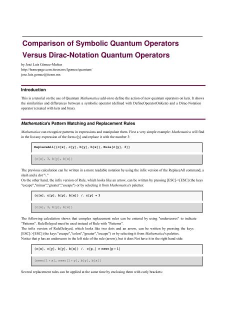
<strong>Comparison</strong> <strong>of</strong> <strong>Symbolic</strong> <strong>Quantum</strong> <strong>Operators</strong><br />
<strong>Versus</strong> <strong>Dirac</strong>-<strong>Notation</strong> <strong>Quantum</strong> <strong>Operators</strong><br />
by José Luis Gómez-Muñoz<br />
http://homepage.cem.itesm.mx/lgomez/quantum/<br />
jose.luis.gomez@itesm.mx<br />
Introduction<br />
This is a tutorial on the use <strong>of</strong> <strong>Quantum</strong> Mathematica add-on to define the action <strong>of</strong> new quantum operators on kets. It shows<br />
the similarities and differences between a symbolic operator (defined with DefineOperatorOnKets) and a <strong>Dirac</strong>-<strong>Notation</strong><br />
operator (created with kets and bras).<br />
Mathematica's Pattern Matching and Replacement Rules<br />
Mathematica can recognize patterns in expressions and manipulate them. First a very simple example: Mathematica will find<br />
in the list any expression <strong>of</strong> the form c[y] and replace it with the number 3:<br />
ReplaceAll@8c@xD, c@yD, b@yD, b@xD[ESC] (the keys<br />
"escape","minus","greater","escape") or by selecting it from Mathematica's palettes:<br />
8c@xD, c@yD, b@yD, b@xD< ê. c@yD → 3<br />
8c@xD, 3, b@yD, b@xD<<br />
The following calculation shows that complex replacement rules can be entered by using "underscores" to indicate<br />
"Patterns". RuleDelayed must be used instead <strong>of</strong> Rule with "Patterns".<br />
The infix version <strong>of</strong> RuleDelayed, which looks like two dots and an arrow, can be written by pressing the keys<br />
[ESC]:>[ESC] (the keys "escape","colon","greater","escape") or by selecting it from Mathematica's palettes.<br />
Notice that p has an underscore in the left side <strong>of</strong> the rule (arrow), but it does Not have it in the right hand side:<br />
8c@xD, c@yD, b@yD, b@xD< ê. c@p_D ⧴ newc@p +1D<br />
8newc@1 +xD, newc@1 +yD, b@yD, b@xD<<br />
Several replacement rules can be applied at the same time by enclosing them with curly brackets:
2 v7defope.nb<br />
8c@xD, c@yD, b@yD, b@xD< ê. 8c@p_D ⧴ newc@p +1D, b@yD → foo@yD<<br />
8newc@1 +xD, newc@1 +yD, foo@yD, b@xD<<br />
It is very important to understand the difference between the previous calculation (where b[x] did not change) and the next<br />
one (where both b[x] and b[y] are changed)<br />
8c@xD, c@yD, b@yD, b@xD< ê. 8c@p_D ⧴ newc@p +1D, b@y_D ⧴ foo@yD<<br />
8newc@1 +xD, newc@1 +yD, foo@yD, foo@xD<<br />
Next the sintaxis <strong>of</strong> replacement rules will be used to create new <strong>Quantum</strong> operators to be used in Mathematica<br />
Load the Package<br />
First load the <strong>Quantum</strong>`<strong>Notation</strong>` package. Write:<br />
Needs["<strong>Quantum</strong>`<strong>Notation</strong>`"]<br />
then press at the same time the keys ˜-Û to evaluate. Mathematica will load the package:<br />
Needs@"<strong>Quantum</strong>`<strong>Notation</strong>`"D<br />
<strong>Quantum</strong>`<strong>Notation</strong>` Version 2.2.0. HJuly 2010L<br />
A Mathematica package for <strong>Quantum</strong> calculations in <strong>Dirac</strong> bra−ket notation<br />
by José Luis Gómez−Muñoz<br />
Execute Set<strong>Quantum</strong>Aliases@D in order to use<br />
the keyboard to enter quantum objects in <strong>Dirac</strong>'s notation<br />
Set<strong>Quantum</strong>Aliases@D must be executed again in each new<br />
notebook that is created, only one time per notebook.<br />
In order to use the keyboard to enter quantum objects write:<br />
Set<strong>Quantum</strong>Aliases[ ];<br />
then press at the same time the keys ˜-Û to evaluate. The semicolon prevents Mathematica from printing the help<br />
message. Remember that Set<strong>Quantum</strong>Aliases[ ] must be evaluated again in each new notebook:<br />
Set<strong>Quantum</strong>Aliases@D;<br />
The Command DefineOperatorOnKets[]<br />
We will use the command DefineOperatorOnKets.<br />
A basic help can be obtained by writting<br />
? DefineOperatorOnKets<br />
then press at the same time the keys ˜-Û to evaluate:
v7defope.nb 3<br />
?DefineOperatorOnKets<br />
DefineOperatorOnKets@op,8rules[ESC]<br />
[ESC]eket[ESC] } ]<br />
then press the [TAB] several times in order to select the first place-holder (empty square) and write:<br />
1 [TAB] q1 [TAB] 2 [TAB] q1 [TAB] 2 [TAB] q1 [TAB] 3 [TAB] q1<br />
then press at the same time the keys ˜-Û to evaluate:<br />
DefineOperatorOnKetsBope1, :<br />
1 ˆ q1<br />
^ →<br />
2 ˆ q1<br />
^, 2 ˆ q1<br />
^ →<br />
3 ˆ q1<br />
^>F<br />
ope1 ⋅<br />
ope1 ⋅<br />
1 ˆ q1<br />
^ →<br />
2 ˆ<br />
q1<br />
^ →<br />
2 ˆ q1<br />
^<br />
3 ˆ<br />
q1<br />
^<br />
Now we can use our new operator.<br />
Write:<br />
ope1 [ESC]on[ESC] (b [ESC]eket[ESC] + c [ESC]eket[ESC] )<br />
then press the [TAB] several times in order to select the first place-holder (empty square) and write:<br />
1 [TAB] q1 [TAB] 2 [TAB] q1<br />
then press at the same time the keys ˜-Û to evaluate:<br />
ope1 ⋅ Jb 1 ˆ q1<br />
^ +c 2 ˆ q1<br />
^N<br />
b 2 ˆ<br />
q1<br />
^ +c 3 ˆ<br />
q1<br />
^<br />
In this simple case, we can use <strong>Dirac</strong> notation to write an operator that does something similar:<br />
dirac1 =<br />
2 q1ˆ ^ ⋅ Z1 ˆ<br />
q1<br />
+ 3 ˆ<br />
q1<br />
^ ⋅ Z2 ˆ<br />
q1<br />
2 ˆ q1<br />
^ ⋅ Z1 ˆ q1<br />
+ 3 ˆ q1<br />
^ ⋅ Z2 ˆ q1<br />
Now in this simple calculation the operators ope1, which was defined with the command DefineOperatorOnKets, and dirac1,<br />
which was created directly from the <strong>Dirac</strong> notation, give the same result:<br />
dirac1 ⋅ Jb 1 ˆ<br />
q1<br />
^ +c 2 ˆ<br />
q1<br />
^N<br />
b 2 ˆ<br />
q1<br />
^ +c 3 ˆ<br />
q1<br />
^<br />
The Mathematica command Column gives a simple way to show both results at the same time:
4 v7defope.nb<br />
ColumnB:<br />
>F<br />
ope1 ⋅ Jb 1 ˆ<br />
q1<br />
^ +c 2 ˆ<br />
q1<br />
^N,<br />
dirac1 ⋅ Jb 1 ˆ<br />
q1<br />
^ +c 2 ˆ<br />
q1<br />
^N<br />
b 2 ˆ q1<br />
^ +c 3 ˆ q1<br />
^<br />
b 2 ˆ<br />
q1<br />
^ +c 3 ˆ<br />
q1<br />
^<br />
The hermitian conjugate (entered as [ESC]her[ESC]) <strong>of</strong> both operators applied to a bra gives the expected answer (Notice<br />
that it is necessary to "Expand" for the hermitian <strong>of</strong> dirac1 on a Bra):<br />
ColumnB:<br />
Z2 ˆ<br />
q1<br />
⋅ Hope1L † ,<br />
Z2 ˆ q1<br />
⋅ Hdirac1L † ,<br />
ExpandBZ2 ˆ<br />
q1<br />
⋅ Hdirac1L † F<br />
>F<br />
Z3 ˆ q1<br />
Z2 ˆ<br />
q1<br />
⋅ J 1 ˆ<br />
q1<br />
^ ⋅ Z2 ˆ<br />
q1<br />
+ 2 ˆ<br />
q1<br />
^ ⋅ Z3 ˆ<br />
q1<br />
N<br />
Z3 ˆ<br />
q1<br />
On the other hand, there are situations where these two operators, created in different ways, are Not equivalent.<br />
As you can see in the following example, when ope1 acts on a ket where its action was not defined, it remains unevaluated.<br />
On the other, dirac1 vanishes that ket:<br />
ColumnB:<br />
>F<br />
ope1 ⋅ Jb 1 ˆ<br />
q1<br />
^ +c 2 ˆ<br />
q1<br />
^ +d 3 ˆ<br />
q1<br />
^N,<br />
dirac1 ⋅ Jb 1 ˆ<br />
q1<br />
^ +c 2 ˆ<br />
q1<br />
^ +d 3 ˆ<br />
q1<br />
^N<br />
dope1 ⋅<br />
3 ˆ<br />
q1<br />
^ +b 2 ˆ<br />
q1<br />
^ +c 3 ˆ<br />
q1<br />
^<br />
b 2 ˆ q1<br />
^ +c 3 ˆ q1<br />
^<br />
Now the important advantage <strong>of</strong> the command DefineOperatorOnKets over the direct <strong>Dirac</strong> definition <strong>of</strong> an operator is the<br />
use <strong>of</strong> the powerful "Pattern" matching capabilities <strong>of</strong> Mathematica. Here we use the "Pattern" (the n with underscore, n_)<br />
and the "RuleDelayed" [ESC]:>[ESC] (the keys "escape","colon","greater","escape") in order to create a powerful "rising"<br />
operator, called ope2.<br />
Notice that n has an underscore in the left side <strong>of</strong> the rule (arrow), but it does Not have it in the right hand side. Notice also<br />
the use <strong>of</strong> parenthesis in (n+1):
v7defope.nb 5<br />
DefineOperatorOnKetsBope2, :<br />
n_ ˆ q1<br />
^ ⧴<br />
Hn +1L ˆ q1<br />
^>F<br />
n_ ˆ q1<br />
^ ⧴<br />
Hn +1L ˆ q1<br />
^<br />
Now we can compare the three rising operators:<br />
ColumnB:<br />
>F<br />
ope1 ⋅ Jb 1 ˆ<br />
q1<br />
^ +c 2 ˆ<br />
q1<br />
^ +d 3 ˆ<br />
q1<br />
^N,<br />
dirac1 ⋅ Jb 1 ˆ<br />
q1<br />
^ +c 2 ˆ<br />
q1<br />
^ +d 3 ˆ<br />
q1<br />
^N,<br />
ope2 ⋅ Jb 1 ˆ<br />
q1<br />
^ +c 2 ˆ<br />
q1<br />
^ +d 3 ˆ<br />
q1<br />
^N<br />
dope1 ⋅<br />
3 ˆ q1<br />
^ +b 2 ˆ q1<br />
^ +c 3 ˆ q1<br />
^<br />
b 2 ˆ q1<br />
^ +c 3 ˆ q1<br />
^<br />
b 2 ˆ<br />
q1<br />
^ +c 3 ˆ<br />
q1<br />
^ +d 4 ˆ<br />
q1<br />
^<br />
It can be created an operator using <strong>Dirac</strong> notation in Mathematica that works the same as ope2:<br />
∞<br />
dirac2 = ‚<br />
j=−∞<br />
Hj +1L ˆ<br />
q1<br />
^ ⋅ Zj ˆ<br />
q1<br />
∞<br />
‚<br />
j=−∞<br />
Hj +1L ˆ q1<br />
^ ⋅ Zj ˆ q1<br />
Here the two operators do the same<br />
ColumnB:<br />
ope2 ⋅ Jb 100 ˆ<br />
q1<br />
^ +c 200 ˆ<br />
q1<br />
^ +d 1020 ˆ<br />
q1<br />
^N,<br />
dirac2 ⋅ Jb 100 ˆ<br />
q1<br />
^ +c 200 ˆ<br />
q1<br />
^ +d 1020 ˆ<br />
q1<br />
^N<br />
>, Dividers → AllF<br />
b 101 ˆ q1<br />
^ +c 201 ˆ q1<br />
^ +d 1021 ˆ q1<br />
^<br />
b 101 ˆ q1<br />
^ +c 201 ˆ q1<br />
^ +d 1021 ˆ q1<br />
^<br />
Powers <strong>of</strong> operators can easily be calculated
6 v7defope.nb<br />
ColumnB:<br />
ope2 4 ⋅ Jb 100 ˆ<br />
q1<br />
^ +c 200 ˆ<br />
q1<br />
^ +d 1020 ˆ<br />
q1<br />
^N,<br />
dirac2 4 ⋅ Jb 100 q1ˆ ^ +c 200 ˆ<br />
q1<br />
^ +d 1020 ˆ<br />
q1<br />
^N<br />
>, Dividers → AllF<br />
b 104 ˆ q1<br />
^ +c 204 ˆ q1<br />
^ +d 1024 ˆ q1<br />
^<br />
b 104 ˆ<br />
q1<br />
^ +c 204 ˆ<br />
q1<br />
^ +d 1024 ˆ<br />
q1<br />
^<br />
Differences between an operator created with DefineOperatorOnKets[] and an operator<br />
created with kets and bras<br />
These are the definitions <strong>of</strong> the two operators we are working with. The operator dirac2 is created from kets and bras, while<br />
the symbolic operator ope2 is created with the <strong>Quantum</strong> Mathematica command DefineOperatorOnKets[]:<br />
Needs@"<strong>Quantum</strong>`<strong>Notation</strong>`"D;<br />
∞<br />
dirac2 = ‚<br />
j=−∞<br />
Hj +1L ˆ<br />
q1<br />
^ ⋅ Zj ˆ<br />
q1<br />
;<br />
DefineOperatorOnKetsBope2, :<br />
n_ ˆ<br />
q1<br />
^ ⧴<br />
Hn +1L ˆ<br />
q1<br />
^>F;<br />
Both have the same effect on a superposition <strong>of</strong> kets:<br />
ColumnB:<br />
ope2 ⋅ Jb 100 ˆ<br />
q1<br />
^ +c 200 ˆ<br />
q1<br />
^ +d 1020 ˆ<br />
q1<br />
^N,<br />
dirac2 ⋅ Jb 100 ˆ<br />
q1<br />
^ +c 200 ˆ<br />
q1<br />
^ +d 1020 ˆ<br />
q1<br />
^N<br />
>, Dividers → AllF<br />
b 101 ˆ q1<br />
^ +c 201 ˆ q1<br />
^ +d 1021 ˆ q1<br />
^<br />
b 101 ˆ q1<br />
^ +c 201 ˆ q1<br />
^ +d 1021 ˆ q1<br />
^<br />
However the hermitian conjugate <strong>of</strong> ope2 has no action on kets, while the hermitian conjugate <strong>of</strong> dirac2 has a very specific<br />
effect:<br />
ColumnB:<br />
Hope2L † ⋅ Jb 100 ˆ<br />
q1<br />
^ +c 200 ˆ<br />
q1<br />
^ +d 1020 ˆ<br />
q1<br />
^N,<br />
Hdirac2L † ⋅ Jb 100 q1ˆ ^ +c 200 ˆ<br />
q1<br />
^ +d 1020 ˆ<br />
q1<br />
^N<br />
>, Dividers → AllF<br />
ope2 † ⋅ Jb 100 ˆ q1<br />
^ +c 200 ˆ q1<br />
^ +d 1020 ˆ q1<br />
^N<br />
b 99 ˆ q1<br />
^ +c 199 ˆ q1<br />
^ +d 1019 ˆ q1<br />
^
v7defope.nb 7<br />
We can force the hermitian conjugate <strong>of</strong> ope2 to have the same effect as the hermitian conjugate <strong>of</strong> dirac2. Notice the use <strong>of</strong><br />
the parenthesis in (n-1)<br />
DefineOperatorOnKetsBHope2L † , :<br />
ColumnB:<br />
n_ ˆ<br />
q1<br />
^ ⧴<br />
Hn −1L ˆ<br />
q1<br />
^>F;<br />
Hope2L † ⋅ Jb 100 ˆ<br />
q1<br />
^ +c 200 ˆ<br />
q1<br />
^ +d 1020 ˆ<br />
q1<br />
^N,<br />
Hdirac2L † ⋅ Jb 100 q1ˆ ^ +c 200 ˆ<br />
q1<br />
^ +d 1020 ˆ<br />
q1<br />
^N<br />
>, Dividers → AllF<br />
b 99 ˆ q1<br />
^ +c 199 ˆ q1<br />
^ +d 1019 ˆ q1<br />
^<br />
b 99 ˆ<br />
q1<br />
^ +c 199 ˆ<br />
q1<br />
^ +d 1019 ˆ<br />
q1<br />
^<br />
Perhaps the main difference between ope2 (created with DefineOperatorOnKets[]) and dirac2 (created with kets and bras) is<br />
what happen when these operators are not acting on kets or bras:<br />
Column@8<br />
ope2,<br />
dirac2<br />
8 v7defope.nb<br />
Set<strong>Quantum</strong>Object@qoD;<br />
ColumnA9<br />
CommutatorExpandAHope2 +qoL 2 E,<br />
CommutatorExpandAHdirac2 +qoL 2 E<br />
=, Dividers → AllE<br />
ope2 2 +qo 2 − Pope2, qoT −<br />
+2ope2 ⋅qo<br />
qo 2 ∞<br />
+ ⁄ j3=−∞<br />
H2 +j3L ˆ q1<br />
^ ⋅ Zj3 ˆ q1<br />
+<br />
∞<br />
⁄ j=−∞<br />
H1 +jL ˆ q1<br />
^ ⋅ Zj ˆ q1<br />
∞<br />
⋅qo + ⁄ j=−∞ qo ⋅ H1 +jL ˆ q1<br />
^ ⋅ Zj ˆ q1<br />
The two expressions above are equivalent, as can be seen when they are applied to the same ket:<br />
Set<strong>Quantum</strong>Object@qoD;<br />
ColumnB:<br />
CommutatorExpandAHope2 +qoL 2 E ⋅<br />
CommutatorExpandAHdirac2 +qoL 2 E ⋅<br />
100 ˆ<br />
q1<br />
^,<br />
100 ˆ<br />
q1<br />
^<br />
>, Dividers → AllF<br />
qo 2 ⋅<br />
100 ˆ q1<br />
^ +qo ⋅<br />
101 ˆ q1<br />
^ +ope2 ⋅qo ⋅<br />
100 ˆ q1<br />
^ +<br />
102 ˆ q1<br />
^<br />
∞<br />
⁄ j=−∞<br />
H1 +jL ˆ<br />
q1<br />
^ ⋅ Zj ˆ<br />
q1<br />
⋅qo ⋅ 100 ˆ<br />
q1<br />
^ +qo 2 ⋅<br />
100 ˆ<br />
q1<br />
^ +qo ⋅<br />
101 ˆ<br />
q1<br />
^ +<br />
102 ˆ<br />
q1<br />
^<br />
by José Luis Gómez-Muñoz<br />
http://homepage.cem.itesm.mx/lgomez/quantum/<br />
jose.luis.gomez@itesm.mx