Sensitivity of the Kurtosis Statistic as a Detector - Remote Sensing ...

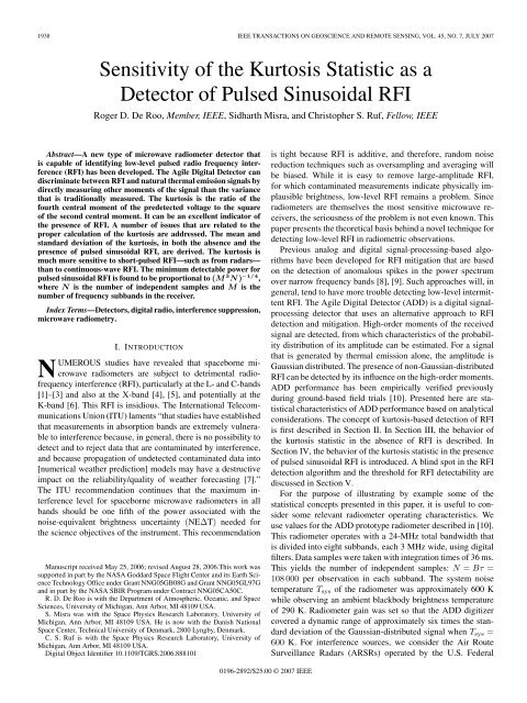
1938 IEEE TRANSACTIONS ON GEOSCIENCE AND REMOTE SENSING, VOL. 45, NO. 7, JULY 2007 

Sensitivity of the Kurtosis Statistic as a 

Detector of Pulsed Sinusoidal RFI 

Roger D. De Roo, Member, IEEE, Sidharth Misra, and Christopher S. Ruf, Fellow, IEEE 

Abstract—A new type of microwave radiometer detector that 

is capable of identifying low-level pulsed radio frequency interference 

(RFI) has been developed. The Agile Digital Detector can 

discriminate between RFI and natural thermal emission signals by 

directly measuring other moments of the signal than the variance 

that is traditionally measured. The kurtosis is the ratio of the 

fourth central moment of the predetected voltage to the square 

of the second central moment. It can be an excellent indicator of 

the presence of RFI. A number of issues that are related to the 

proper calculation of the kurtosis are addressed. The mean and 

standard deviation of the kurtosis, in both the absence and the 

presence of pulsed sinusoidal RFI, are derived. The kurtosis is 

much more sensitive to short-pulsed RFI—such as from radars— 

than to continuous-wave RFI. The minimum detectable power for 

pulsed sinusoidal RFI is found to be proportional to (M 3 N ) −1/4 , 

where N is the number of independent samples and M is the 

number of frequency subbands in the receiver. 

Index Terms—Detectors, digital radio, interference suppression, 

microwave radiometry. 

I. INTRODUCTION 

NUMEROUS studies have revealed that spaceborne microwave 

radiometers are subject to detrimental radiofrequency 

interference (RFI), particularly at the L- and C-bands 

[1]–[3] and also at the X-band [4], [5], and potentially at the 

K-band [6]. This RFI is insidious. The International Telecommunications 

Union (ITU) laments “that studies have established 

that measurements in absorption bands are extremely vulnerable 

to interference because, in general, there is no possibility to 

detect and to reject data that are contaminated by interference, 

and because propagation of undetected contaminated data into 

[numerical weather prediction] models may have a destructive 

impact on the reliability/quality of weather forecasting [7].” 

The ITU recommendation continues that the maximum interference 

level for spaceborne microwave radiometers in all 

bands should be one fifth of the power associated with the 

noise-equivalent brightness uncertainty (NE∆T) needed for 

the science objectives of the instrument. This recommendation 

Manuscript received May 25, 2006; revised August 28, 2006.This work was 

supported in part by the NASA Goddard Space Flight Center and its Earth Science 

Technology Office under Grant NNG05GB08G and Grant NNG05GL97G 

and in part by the NASA SBIR Program under Contract NNG05CA50C. 

R. D. De Roo is with the Department of Atmospheric, Oceanic, and Space 

Sciences, University of Michigan, Ann Arbor, MI 48109 USA. 

S. Misra was with the Space Physics Research Laboratory, University of 

Michigan, Ann Arbor, MI 48109 USA. He is now with the Danish National 

Space Center, Technical University of Denmark, 2800 Lyngby, Denmark. 

C. S. Ruf is with the Space Physics Research Laboratory, University of 

Michigan, Ann Arbor, MI 48109 USA. 

Digital Object Identifier 10.1109/TGRS.2006.888101 

is tight because RFI is additive, and therefore, random noise 

reduction techniques such as oversampling and averaging will 

be biased. While it is easy to remove large-amplitude RFI, 

for which contaminated measurements indicate physically implausible 

brightness, low-level RFI remains a problem. Since 

radiometers are themselves the most sensitive microwave receivers, 

the seriousness of the problem is not even known. This 

paper presents the theoretical basis behind a novel technique for 

detecting low-level RFI in radiometric observations. 

Previous analog and digital signal-processing-based algorithms 

have been developed for RFI mitigation that are based 

on the detection of anomalous spikes in the power spectrum 

over narrow frequency bands [8], [9]. Such approaches will, in 

general, tend to have more trouble detecting low-level intermittent 

RFI. The Agile Digital Detector (ADD) is a digital signalprocessing 

detector that uses an alternative approach to RFI 

detection and mitigation. High-order moments of the received 

signal are detected, from which characteristics of the probability 

distribution of its amplitude can be estimated. For a signal 

that is generated by thermal emission alone, the amplitude is 

Gaussian distributed. The presence of non-Gaussian-distributed 

RFI can be detected by its influence on the high-order moments. 

ADD performance has been empirically verified previously 

during ground-based field trials [10]. Presented here are statistical 

characteristics of ADD performance based on analytical 

considerations. The concept of kurtosis-based detection of RFI 

is first described in Section II. In Section III, the behavior of 

the kurtosis statistic in the absence of RFI is described. In 

Section IV, the behavior of the kurtosis statistic in the presence 

of pulsed sinusoidal RFI is introduced. A blind spot in the RFI 

detection algorithm and the threshold for RFI detectability are 

discussed in Section V. 

For the purpose of illustrating by example some of the 

statistical concepts presented in this paper, it is useful to consider 

some relevant radiometer operating characteristics. We 

use values for the ADD prototype radiometer described in [10]. 

This radiometer operates with a 24-MHz total bandwidth that 

is divided into eight subbands, each 3 MHz wide, using digital 

filters. Data samples were taken with integration times of 36 ms. 

This yields the number of independent samples: N = Bτ = 

108 000 per observation in each subband. The system noise 

temperature T sys of the radiometer was approximately 600 K 

while observing an ambient blackbody brightness temperature 

of 290 K. Radiometer gain was set so that the ADD digitizer 

covered a dynamic range of approximately six times the standard 

deviation of the Gaussian-distributed signal when T sys = 

600 K. For interference sources, we consider the Air Route 

Surveillance Radars (ARSRs) operated by the U.S. Federal 

0196-2892/$25.00 © 2007 IEEE

DE ROO et al.: SENSITIVITY OF THE KURTOSIS STATISTIC 1939 

signal, higher order moments are uniquely determined by the 

standard deviation. The kurtosis of v is defined as 

R = m 4 

m 2 . (3) 

2 

Fig. 1. Example of predetection signals. On the left are time-domain representations 

of the signals. Their pdfs are shown on the right. Geophysical signals 

and receiver noise are Gaussian distributed in amplitude (top), while sinusoids 

have a distinctly non-Gaussian pdf (bottom). 

Aviation Administration. These L-band radars are distributed 

throughout the U.S. and transmit at megawatt peak power levels 

with center frequencies that range from 1215–1380 MHz [11], 

which is very close to the L-band passive band in the range 

of 1400–1427 MHz. ARSR-1 radars transmit with a 0.072% 

duty cycle, while ARSR-4 radars transmit with a 1%–3.24% 

duty cycle. 

II. PRINCIPLE OF KURTOSIS-BASED RFI DETECTION 

IN MICROWAVE RADIOMETRY 

The signal detected by a microwave radiometer is primarily 

from natural thermal emission as well as thermal noise generated 

by the hardware. The probability density function (pdf) 

of the amplitude of this signal is Gaussian distributed. The 

most likely form of RFI is sinusoidal, which has a completely 

different amplitude distribution, as shown in Fig. 1. 

In the absence of RFI, the random voltage v at the input 

to a digitizer is given by the Gaussian probability density 

p g (v), i.e., 

p g (v) = 1 

σ √ 2π e −v2 

2σ 2 . (1) 

The RFI detection algorithm makes use of the higher order 

moments of the random variable v. The central moments of the 

distribution are given by 

m g n = 〈(v −〈v〉) n 〉 =1· 3 ······(n − 1)σ n (2) 

where σ is the standard deviation of v and n is even. The moment 

m n =0when n is odd. In case of a Gaussian-distributed 

For a Gaussian-distributed signal, the kurtosis is equal to 3, 

independent of σ. In case the signal is corrupted by RFI, the 

probability may deviate from a Gaussian distribution, and the 

value of the kurtosis may deviate from 3. 

The detection of RFI thus reduces to the problem of deciding 

from its samples if a variable is normally distributed. This 

is a well-documented area of research [12]. The momentratio-based 

methods are especially appealing for radiometric 

operation because calculations of the test statistic are simple 

(and therefore fast), they do not require significant data storage 

(e.g., no ranking of data is required), and the postdetect data 

transmission rate is not significantly different from current 

receiver technologies that do not employ RFI detection. In 

addition, the statistic R is independent of the statistic m 2 for 

a Gaussian distribution [12]. Therefore, estimates of m 2 and 

hence of the brightness temperature will be unbiased by the 

removal of samples incorrectly flagged as containing RFI by a 

kurtosis-based algorithm. RFI detection algorithms which rely 

on brightness thresholds may be biased because high outliers 

are suppressed. 

III. KURTOSIS IN THE ABSENCE OF RFI 

While the kurtosis is ideally equal to 3 for a Gaussian distribution, 

the measurement process results in a sample estimate 

of the kurtosis that can deviate from the theoretical value. This 

section explores some mechanisms of the measurement process 

and how they can affect the estimate of the kurtosis when no 

RFI is present. 

A. Effects of Finite Number of Independent Samples 

Because the kurtosis is estimated from a finite sample set, it 

is itself a random variable. Let its pdf be denoted by p(R; N), 

where N is the number of independent samples. The area under 

the outlying tails of the pdf determines the rate of false detections 

of RFI in otherwise RFI-free radiometric observations. 

Closed-form expressions for p(R; N) exist only for N =4 

[13], which is a sample size that is much too small for practical 

utility. Fortunately, the moments of p(R; N) are known 

exactly for arbitrary N up to the seventh moment [14]–[16] 

and can be used to estimate the area under its tails. In the 

limit of large N, p(R; N) tends toward normal with mean 

〈R〉 =3(N − 1)/(N +1) and variance that asymptotically 

approaches 24/N . The normal approximation requires a rather 

large N (N >50 000). For radiometer applications with very 

fine bandwidth resolution and very short integration times, the 

non-Gaussian nature of p(R; N) should be taken into account 

in order to minimize the false alarms of RFI detection. 

A common moment-based estimator for pdfs and cumulative 

distribution functions (CDFs) is the Edgeworth series [17], 

but this series generates negative values for the pdf in the 

tails, resulting in poor area estimates under the tails. Bowman


TABLE I 

RATIO OF SAMPLES WITHIN THE DIGITIZER SPAN TO OUTLIERS FOR AN 

RFI-FREE SIGNAL WITH DIFFERENT DIGITIZER SPANS 

3.279. While the RFI-free rejection is about the same (1.1%), 

the actual 1% thresholds are 2.744


of the moments about the origin can be readily derived with the 

binomial formula [21] 

m a 2 = µ 2 − µ 2 1 (6) 

m a 4 = µ 4 − 4µ 3 µ 1 +6µ 2 µ 2 1 − 3µ 4 1 (7) 

where the superscript a indicates an ideal analog operation, 

i.e., without the effects of digitization. Thus, a digital receiver 

configured to perform kurtosis calculations should collect the 

first four moments about the origin of the data to correct for the 

ADC null offset. Null offsets of even a fraction of a digitizing 

bin can be removed in this manner. 

D. Effects of Digitization 

Digitization of the signal results in a small loss of information 

since the continuous random variable is binned by the 

ADC. For example, the variance of a digitized Gaussian signal 

is larger than the variance of the analog signal by the variance 

of a uniform distribution that is one digitizing bin wide. This 

is because the act of digitizing can be viewed as adding to 

the analog signal a random amount, which is either positive 

or negative up to one half of a digitizing bin. If the signal 

strength is sufficiently strong, the amount added to the data 

by digitization is nearly uniformly distributed. A similar effect 

occurs to all even moments of a digitized distribution. Fischman 

and England [22] have derived the effects of digitization on the 

moments of a Gaussian distribution as a function of the width 

of a digitization bin v 0 . They found that 

m d 2 = σ 2 + 1 

12 v2 0 (8) 

m d 4 =3σ 4 + 1 2 σ2 v 2 0 + 1 80 v4 0 (9) 

where the superscript d indicates that the Gaussian signal has 

been digitized. They further found that the correction for the 

variance is accurate for a Gaussian signal as long as the standard 

deviation σ is greater than 2/3 v 0 and the correction for the 

fourth moment is accurate for σ>3/4 v 0 . 

For radio brightness measurements of the second moment, 

this digitization offset is a constant and can be lumped with 

the receiver temperature. For kurtosis measurements of thermal 

noise, the digitization offsets in the second and fourth moments 

nearly cancel when the ratio (3) is taken, i.e., 

m d 4 

( 

m 

d 

2 

) 2 

=3− 

1 

120 

( ( 

σ 

v 0 

) 2 

+ 

1 

12 

) 2 

. (10) 

The offset induced in the kurtosis statistic by neglecting the 

effects of digitization is always negative, and while it is about 

−1% at σ =2/3 v 0 , it decreases to −0.24% at σ = v 0 and 

decreases further as the signal strength at the ADC input is 

increased. For the case of the ADD measurements presented 

in [10], the instrument gain was set so that σ =10v 0 . 

The correction for the effects of digitization has been derived 

by Sheppard and is given by [21] 

m 2 = µ 2 − µ 2 1 − 1 

12 v2 0 

m 4 = µ 4 − 4µ 3 µ 1 +6µ 2 µ 2 1 − 3µ 4 1 

− 1 ( 

µ2 − µ 2 

2 

1) 

v 

2 

0 + 7 

240 v4 0. (11) 

These moments are the estimators of the second and fourth 

central moments, which are unbiased by the effects of digitization, 

in terms of the output of the FPGA. Errors in the 

ADC transfer function measured by the differential and integral 

nonlinearities have not been considered. While radiometric and 

even interferometric operation is quite feasible with only a few 

levels, Sheppard’s correction must be generalized for optimal 

signal detection [23]. In the rest of this paper, our measurements 

were made with sufficiently strong signals that Sheppard’s 

correction has been neglected. 

IV. KURTOSIS IN THE PRESENCE OF 

PULSED SINUSOIDAL RFI 

The kurtosis may change in the presence of RFI. Here, we 

characterize the behavior of the kurtosis in the presence of a 

radarlike source of RFI. 

A. Combined Gaussian Noise and a Pulsed Sinusoid 

Assume that the RFI can be modeled as a pulsed sinusoid 

with an amplitude A and total duration dτ, where τ is the 

radiometer integration time and 0 ≤ d ≤ 1. In our case, even 

though the RFI is deterministic in nature, we consider its 

amplitude histogram as an equivalent probability distribution. 

The pdf of such a waveform is given by 

d 

p ps (v) =(1− d)δ(v)+ 

π √ (12) 

A 2 − v 2 

where δ(x) is the Dirac delta function. If the integration time 

greatly exceeds the interpulse period, then d is the radar’s 

duty cycle, which is the proportion of time that the radar 

is transmitting. We require the probability distribution of the 

combined signal that includes both thermal emission and the 

RFI signal. Rice [24] determined the probability distribution 

function for the instantaneous voltage of a sinusoid with noise, 

which is easily extended to the case of a pulsed sinusoid, i.e., 

p(v) = 1 √ 

2πσ 

e −v2 

2σ 2 (1+d 

where 

He 2k (x) = 

k∑ 

m=0 

∞∑ 

( ) 2k 

1 A 

( v 

) ) 

(k!) 2 He 2k 

2σ σ 

(13) 

k=1 

(−1) m 

2 m (2k)! 

m!(2k − 2m)! x2k−2m (14) 

is a Hermite polynomial of even order [17]. When d =0 

or A =0, the expression reduces to a Gaussian probability


Fig. 3. Instantaneous voltage pdf for constant Gaussian noise level and 

constant pulsed sinusoid amplitude but varying duty cycle. 

Fig. 5. Examples of instantaneous voltage pdfs with the same variance 

(m ps 

2 = 64). Pulsed sinusoidal RFI, when present, has a constant signal-tonoise 

power level but different duty cycles. The low-duty-cycle RFI has the 

highest tails and is easiest to detect with the kurtosis statistic. 

where S is the signal-to-noise ratio of the pulsed sinusoid power 

(P ps = dA 2 /2, which is averaged over an integration period) to 

the noise power and is given by 

S = dA2 

2σ 2 = P ps 

kT sys B = T ps 

T sys 

(19) 

where σ 2 = kT sys B, k is the Boltzmann constant, and B is 

the RF bandwidth. S is also the ratio of the equivalent RFI 

brightness temperature T ps to the system temperature (in the 

absence of RFI) T sys . The shape of the pdf of the instantaneous 

voltage as a function of the duty cycle, but with the total power 

kept constant, is depicted in Fig. 5. The tails of the distribution 

are highest at low duty cycles. 

Fig. 4. Comparison of (13) with the ADD output while the radiometer is 

observing the sky with an equivalent of 2000 K of CW at 1412 MHz added 

to the input. 

distribution. Rice’s result is the case when d =1.Fig.3shows 

the shapes predicted by (13) for constant noise and pulsed 

sinusoid amplitudes. Fig. 4 shows a comparison of Rice’s result 

with the measurements presented in [10]. 

In order to calculate the statistical behavior of the kurtosis, 

we require the first four moments of the resultant signal. Since 

the distributions are symmetric about v =0, the odd moments 

are zero. Thus, the first four nonzero moments for the signal 

with pulsed sinusoidal contamination become 

m ps 

2 = σ2 + dA2 

2 =σ2 (1+S) (15) 

( 

( 

m ps 

4 =3 σ 4 +dA 2 σ 2 + 

)=3σ dA4 4 1+2S+ 1 ) 

8 

2d S2 (16) 

( 

m ps 

6 =5σ6 3+9S+ 9 

2d S2 + 2 ) 

(2d) 2 S3 (17) 

m ps 

8 =35σ8 ( 

3+12S+ 18 

2d S2 + 8 

(2d) 2 S3 + 1 

(2d) 3 S4 ) 

(18) 

B. Mean and Variance of Kurtosis With Pulsed Sinusoidal RFI 

In the presence of pulsed sinusoidal RFI, the large sample 

expected value of the kurtosis becomes 

R(S, d) = 

mps 4 

(m ps 

( 

1+2S + 

1 

=3 2d S2) 

2 )2 (1 + S) 2 . (20) 

In the CW limit (d =1), R ranges from 3 to 3/2 as the power 

in the sinusoid increases. However, as d → 0 but S>0 (corresponding 

to very short radar pulses), R>3. These departures 

from 3 enable the detection of RFI. 

The large sample variance in the kurtosis statistic can be 

derived from the moments to be [25] 

σR(S, 2 1 

d) = 

N (m ps 

2 )4 

[ 

] 

× m ps 

8 − (mps 4 )2 + 4(mps 4 )3 4 mps 6 

. (21) 

4mps 

(m ps − 

2 )2 m ps 

2 

For S =0(i.e., in the absence of RFI), the variance of the kurtosis 

statistic reduces to σR 2 (S =0)=24/N . We shall denote 

this special value as σR0 2 .


V. L IMITS OF DETECTION 

A. Blind Spot and False Alarm Rate (FAR) 

If the kurtosis becomes 3, then, in spite of the presence of 

RFI, the algorithm will fail to detect it. This indicates a blind 

spot in the algorithm. Two conditions are possible in which 

the kurtosis becomes 3: S =0or d =1/2. The first condition 

corresponds to the absence of RFI, while the second is an 

algorithm blind spot. It is worth noting that practical radars tend 

to operate with duty cycles well below 50%, and so radiometers 

will generally not be subject to this problem. Nonetheless, this 

result is somewhat surprising given the obvious differences 

between the 50% duty cycle and Gaussian pdfs in Fig. 5. This 

is because the kurtosis is just one more parameter that describes 

the pdf. A more complete description of the pdf requires more 

moments of the pdf. 

In light of the variance in R even in the absence of RFI, 

there will be a range of RFI around R =3± zσ R0 for some z 

determined by the desired FAR for which the kurtosis algorithm 

is blind. To determine this region of blindness, we solve (20) for 

the duty cycle, i.e., 

d = 

3 

2 S2 

(1 + S) 2 R − 3(1 + 2S) . (22) 

Provided that the number of independent samples N is sufficiently 

high to invoke the normal distribution of the kurtosis R, 

the relation between a specified FAR and the threshold values of 

the kurtosis R tha =3+z a σ R0 and R thb =3− z b σ R0 is given 

by FAR = FAR a + FAR b , where 

FAR a,b = 1 2 

( 

1 − erf(z a,b / √ ) 

2) 

(23) 

and the subscripts a and b refer to the tail of the distribution 

“above” and “below” the RFI-free kurtosis mean value of 3. 

Fig. 6 illustrates the region of sinusoid amplitude and duty 

cycle in which the signal will not be detected by the kurtosis for 

a given number of independent samples and FAR. The kurtosis 

is blind at a 50% duty cycle. In this example, the FAR is nearly 

symmetric (FAR a = FAR b ) because N is sufficiently large to 

invoke the normal distribution of R and z = z a = z b .Forthe 

curves presented in Fig. 6, zσ R0 =0.03, which corresponds 

to an arbitrarily chosen FAR =4.4% for N = 108 000. Under 

these conditions, the 100% duty cycle (CW) limit of detection 

is S = −7.84 dB, corresponding to T ps =99K, assuming an 

RFI-free T sys = 600 K. The limit of detection for very short 

duty cycle RFI is lower. For example, the ∼1% duty cycle of 

ARSR-4 radars should be detectable at −18.4 dB (8.3 K), and 

the ∼0.1% duty cycle of ARSR-1 radars should be detectable 

at S = −23.4 dB (2.7 K) at FAR =4.4%. ForFAR a = 10%, 

the ARSR-1 detectable limit is S = −24.4 dB (2.2 K). Thisis 

very close to the ideal radiometric uncertainty since NE∆T = 

T sys / √ N =1.8 K. 

B. Probability of Detection 

When the number of samples N is sufficiently large to 

describe the distribution of the kurtosis as having a Gaussian 

Fig. 6. Kurtosis blindness to pulsed sinusoidal RFI, with zσ R0 =0.03, 

which is the 4.4% FAR for Bτ = 108 000. The pulsed sinusoidal RFI with 

duty cycle and power between the R =3± zσ R0 curves are not detectable. 

At any power level, a 50% duty cycle is undetectable. The limit of detectability 

for very short pulsed RFI is much lower than that for CW RFI and approaches 

NE∆T. 

distribution with mean R and standard deviation σ R , we can 

predict not only the FAR but also the probability of detection 

(PD) for a given threshold value of kurtosis R th , strength S, and 

duty cycle d of pulsed sinusoid RFI. Considering the blind spot 

at d =1/2, the PD for RFI with d1/2 (e.g., CW RFI) will be denoted as PD b because 

we expect R to be below 3. These probabilities of detection are 

given as 

PD a,b = 1 2 

( ( (Rtha,b 

1 ∓ erf − R(S, d) ) / √ )) 

2σ R (S, d) . 

(24) 

Figs. 7 and 8 show the receiver operating characteristic charts 

for 0.1% and 1% duty cycles, respectively, while Fig. 9 shows 

the same for 100% duty cycle, for a fixed N = 108 000. The 

performance of the algorithm is much better at a low duty cycle. 

C. Dependence of Detection of RFI on System Parameters 

For a duty cycle d that is small, the sinusoid amplitude A 

must be substantial to obtain a particular level of interference. 

The digitizer must not clip this short duration pulse, or we 

will effectively reduce the interference to the point where it 

remains present but is not detectable. If we arbitrarily consider 

the minimum T ps which is unambiguously detectable without 

using the kurtosis statistic as being equal to, say, 10NE∆T, then 

the digitizer should not clip the signal for S


Fig. 7. Probability of detection of a pulsed sinusoid with 0.1% duty cycle 

versus single-sided FAR. N = 108 000. At an RFI contribution equal to 

2NE∆T, detection exceeds 90% for a FAR of 3%. 

Fig. 9. Probability of detection of a CW tone (duty cycle of 100%) versus 

single-sided FAR. N = 108 000. The power in the sinusoid must get relatively 

strong to be reliably detected in a single look. 

Fig. 8. Probability of detection of a pulsed sinusoid with 1% duty cycle versus 

single-sided FAR. N = 108 000. The detection of RFI at a strength of 8NE∆T 

is nearly perfect. 

setting the PD to PD =1− FAR. This is equivalent to setting 

the threshold kurtosis value to the same number of standard 

deviations away from the means of both the RFI-free and pulsed 

sinusoidal RFI-containing pdfs, i.e., 

R tha,b =3− zσ R0 = R(S min ,d)+zσ R (S min ,d) (25) 

where S min is the minimum detectable S and z is a parameter 

that is fixed based on the desired FAR. For example, 

FAR b,a =15.87% for z = ±1, FAR b,a =2.28% for z = ±2, 

Fig. 10. Minimum detectable RFI as a function of the number of samples 

N and duty cycle d for a fixed FAR and PD, with PD =1− FAR, and 

the FAR determined by the threshold kurtosis R th =3± zσ R0 .ForN> 

100 000, the kurtosis algorithm is most sensitive to short duty cycle RFI. The 

minimum detectable RFI, when measured in Kelvin, is proportional to N −1/4 

for a large N. 

and FAR b,a =0.13% for z = ±3. Solving the equation for the 

constant z, we get 

√ ( ) 

3Smin 

2 N 

24 1 − 

1 

2d 

z = 

(1 + S min ) 2 (1 + σ R (S min ,d)/σ R0 ) . (26) 

As N →∞, the ratio of the standard deviations becomes 

constant, and S min is proportional to N −1/4 . Expressed in 

terms of the ideal radiometer uncertainty NE∆T, which itself 

is proportional to N −1/2 , the minimum detectable RFI grows 

as N 1/4 , as shown in Fig. 10. Thus, the kurtosis algorithm can 

be used to detect an arbitrarily low level of RFI, but the number


of samples needed to do so increases somewhat faster than that 

needed for a particular radiometric resolution. 

Division of the RF bandwidth B into subbands is an approach 

to salvage some observations when the RFI is narrowband 

and has been used to detect RFI by comparing the power 

in each subband [8], [9]. Polyphase filters [26] can be used 

in the FPGA to divide the RF bandwidth into M subbands. 

This division into subbands also enhances the sensitivity of 

the kurtosis statistic to RFI. Because the RFI is presumed to 

be narrowband, the RFI signal strength for a subband with 

pulsed sinusoidal RFI is the same as that which would appear 

in the full reception bandwidth. However, the noise power is 

proportional to the bandwidth, and so the signal-to-noise ratio 

for the subband S sb is enhanced by a factor of M over that 

of full bandwidth reception: S sb = MS. At the same time, 

the number of independent samples for each subband N sb is 

reduced by a factor of M : N sb = N/M. Since the sensitivity 

analysis for one subband is the same as for full-band reception, 

we can conclude that S sb,min is proportional to N −1/4 

sb 

,orfor 

the entire system, S min is proportional to (M 3 N) −1/4 . Thus, 

in terms of the minimum detectable RFI, the division of the 

received bandwidth into eight subbands, as done in the ADD, 

is equivalent to increasing the number of independent samples 

by a factor of 512 and reducing the minimum detectable RFI 

power by a factor of 4.75. 

The limit of detection is a function of S, which is the ratio 

of the pulsed sinusoid power to the total Gaussian-distributed 

power. This Gaussian-distributed power is the system temperature 

T sys , which is the sum of the receiver noise temperature 

and the geophysical brightness temperature, which is the point 

of the radiometric observation, i.e., T sys = T REC + T B .Areduction 

of the receiver noise figure, i.e., a reduction of T REC ,is 

well known to reduce the standard error of observation of T B . 

A quiet receiver also helps in the detection of RFI by reducing 

the T sys , the baseline from which the minimum detectible RFI 

power is calculated from the sinusoid to thermal power ratio S. 

The standard error of the brightness observation can be 

reduced by combining observations together. The same can 

be done, at least in principle, to the other moments of the 

observation, thereby increasing the number of independent 

samples, and thus the sensitivity of the kurtosis test for RFI. 

However, much like the brightness uncertainty can increase for 

long integration times due to gain fluctuations or ultimately, 

scene brightness changes, the kurtosis is also sensitive to these 

effects. For example, if an RFI-free observation has a standard 

deviation σ 1 for a duration t 1 but then suddenly changes to σ 2 

for a duration t 2 , then m 2 =(t 1 σ1 2 + t 2 σ2)/(t 2 1 + t 2 ), and 

m 4 =3(t 1 σ1 4 + t 2 σ2)/(t 4 1 + t 2 ). Thus 

( ) 

R =3 t2 1σ1 4 + t 1 t 2 σ 

4 

1 + σ2 

4 + t 

2 

2 σ2 

4 

t 2 1 σ4 1 + t 1t 2 (2σ1 2 . (27) 

σ2 2 )+t2 2 σ4 2 

In this circumstance, R =3only if σ 1 = σ 2 , t 1 =0,ort 2 =0, 

which are the conditions that correspond to a constant standard 

deviation. Otherwise, R>3. Thus, integration periods should 

be restricted to limit the effects of gain and brightness changes 

on the kurtosis statistic as well as their effects on the brightness. 

VI. CONCLUSION 

The kurtosis of the predetected voltage has been presented 

as a means of detecting the presence of pulsed sinusoidal RFI 

in radiometric observations. The predetected voltage due to 

thermal emission obeys the Gaussian pdf, for which the kurtosis 

is 3, regardless of the variance (brightness) of the signal. Finite 

sample sizes, digitizer offsets, digitizer spans, and the digitizer 

bin size affect the kurtosis calculation in small but predictable 

ways in the absence of RFI. When pulsed sinusoidal RFI is 

added to the thermal noise, the kurtosis statistic can deviate 

significantly from 3, indicating the presence of the RFI. CW 

RFI tends to drive the kurtosis value to less than 3, while short 

duty cycle pulses, such as those from radars, drive the kurtosis 

to exceed 3. A pulsed sinusoid with a 50% duty cycle added to 

Gaussian noise has an expected kurtosis of 3 and thus cannot 

be detected by an RFI detection algorithm using the kurtosis. 

For very short duty cycle RFI, such as radar transmissions, the 

minimum RFI power for which the kurtosis can detect the RFI 

approaches the ideal radiometric uncertainty. The sensitivity of 

the kurtosis to RFI can be enhanced by dividing the system 

bandwidth in the receiver into multiple frequency subbands, 

possibly to the point that some RFI at the limit recommended 

by the ITU for spaceborne passive sensors is detectable. The 

ADD has been configured to use the RFI detection scheme 

based on the kurtosis of the predetected voltage. The ADD has 

been used in multiple campaigns to date, and the data collected 

is currently being processed to demonstrate the performance of 

the RFI detection scheme using the kurtosis. 

REFERENCES 

[1] L. Li, E. G. Njoku, E. Im, P. Change, and K. S. Germain, “A preliminary 

survey of radio-frequency interference over the U.S. in Aqua AMSR-E 

data,” IEEE Trans. Geosci. Remote Sens., vol. 42, no. 2, pp. 380–390, 

Feb. 2004. 

[2] E. G. Njoku, P. Ashcroft, T. K. Chan, and L. Li, “Global survey 

and statistics of radio-frequency interference in AMSR-E land observations,” 

IEEE Trans. Geosci. Remote Sens., vol. 43, no. 5, pp. 938–947, 

May 2005. 

[3] D. M. Le Vine and M. Haken, “RFI at L-band in synthetic aperture 

radiometers,” in Proc. IGARSS, Toulouse, France, Jul. 21–25, 2003, vol. 3, 

pp. 1742–1744. 

[4] S. W. Ellingson and J. T. Johnson, “A polarimetric survey of radiofrequency 

interference in C- and X-bands in the continental United States 

using WindSat radiometry,” IEEE Trans. Geosci. Remote Sens., vol. 44, 

no. 3, pp. 540–549, Mar. 2003. 

[5] L. Li, P. W. Gaiser, M. H. Bettenhausen, and W. Johnson, “WindSat 

radio-frequency interference signature and its identification over land and 

ocean,” IEEE Trans. Geosci. Remote Sens., vol. 44, no. 3, pp. 530–539, 

Mar. 2003. 

[6] M. Younis, J. Maurer, J. Fortuny-Guasch, R. Schneider, W. Wiesbeck, and 

A. J. Gasiewski, “Interference from 24-GHz automotive radars to passive 

microwave Earth remote sensing satellites,” IEEE Trans. Geosci. Remote 

Sens., vol. 42, no. 7, pp. 1387–1389, Jul. 2003. 

[7] International Telecommunications Union, Interference Criteria for Satellite 

Passive Remote Sensing, 2003, Geneva, Switzerland. ITU Recommendation 

ITU-R RS.1029-2. 

[8] A. J. Gasiewski, M. Klein, A. Yevgrafov, and V. Leuski, “Interference 

mitigation in passive microwave radiometry,” in Proc. IGARSS, Toronto, 

ON, Canada, 2002, vol. 3, pp. 1682–1684. 

[9] J. T. Johnson, G. A. Hampson, and S. W. Ellingson, “Design and demonstration 

of an interference suppressing microwave radiometer,” in Proc. 

IGARSS, Anchorage, AK, 2004, pp. 1683–1686. 

[10] C. Ruf, S. M. Gross, and S. Misra, “RFI detection and mitigation for 

microwave radiometry with an agile digital detector,” IEEE Trans. Geosci. 

Remote Sens., vol. 44, no. 3, pp. 694–706, Mar. 2006.


[11] Federal Aviation Administration, Spectrum Management Regulations and 

Procedures Manual, FAA Order 6050.32A, May 1, 1998. 

[12] R. B. D’Agostino and M. A. Stephens, Goodness-of-Fit Techniques. 

New York: Marcel Dekker, 1986. 

[13] A. T. McKay, “The distribution of beta_2 in samples of 4 from a normal 

universe,” Biometrika, vol. 25, no. 3/4, pp. 411–415, Dec. 1933. 

[14] E. S. Pearson, “Note on tests for normality,” Biometrika, vol. 22, no. 3/4, 

pp. 423–424, May 1931. 

[15] C. T. Hsu and D. N. Lawley, “The derivation of the fifth and sixth moments 

of the distribution of b2 in samples from a normal population,” 

Biometrika, vol. 31, no. 3/4, pp. 238–248, Mar. 1940. 

[16] R. C. Geary and J. P. G. Worlledge, “On the computation of universal 

moments of tests of statistical normality derived from samples drawn at 

random from a normal universe,” Biometrika, vol. 34, no. 1/2, pp. 98–110, 

Jan. 1947. 

[17] M. Abramowitz and I. A. Stegun, Handbook of Mathematical Functions. 

Washington, DC: Nat. Bureau Standards, 1964. 

[18] K. O. Bowman and L. R. Shenton, “Omnibus test contours for departures 

from normality based on sqrt(b1) and b2,” Biometrika, vol. 62, no. 2, 

pp. 243–250, Aug. 1975. 

[19] N. L. Johnson, “Tables to facilitate fitting S_U frequency curves,” 

Biometrika, vol. 52, no. 3/4, pp. 547–558, 1965. 

[20] R. B. D’Agostino and E. S. Pearson, “Tests for departures from normality. 

Empirical results for the distributions of b2 and sqrt(b1),” Biometrika, 

vol. 60, no. 3, pp. 613–622, Dec. 1973. 

[21] S. Dawson, An Introduction to the Computation of Statistics. London, 

U.K.: Univ. London Press, 1933. 

[22] M. A. Fischman and A. W. England, “Sensitivity of a 1.4 GHz directsampling 

digital radiometer,” IEEE Trans. Geosci. Remote Sens., vol. 37, 

no. 5, pp. 2172–2180, Sep. 1999. 

[23] C. S. Ruf, “Digital correlators for synthetic aperture interferometric 

radiometry,” IEEE Trans. Geosci. Remote Sens., vol. 33, no. 5, pp. 1222– 

1229, Sep. 1995. 

[24] S. O. Rice, “Statistical properties of a sine wave plus random noise,” Bell 

Syst. Tech. J., vol. 27, no. 1, pp. 109–157, Jan. 1948. 

[25] M. G. Kendall, Advanced Theory of Statistics, 5th ed. New York: Hafner, 

1952. 

[26] F. J. Harris, Multirate Signal Processing for Communication Systems. 

Upper Saddle River, NJ: Prentice-Hall, 2004. 

Roger D. De Roo (S’88–M’96) received the B.S. degree 

in letters and engineering from Calvin College, 

Grand Rapids, MI, in 1986, and the B.S.E., M.S.E., 

and Ph.D. degrees in electrical engineering from the 

University of Michigan, Ann Arbor, in 1986, 1989, 

and 1996, respectively. His dissertation topic was on 

the modeling and measurement of bistatic scattering 

of electromagnetic waves from rough dielectric 

surfaces. 

From 1996 to 2000, he was a Research Fellow 

with the Radiation Laboratory, Department of Electrical 

Engineering and Computer Science, University of Michigan, where he 

investigated the modeling and simulation of millimeter-wave backscattering 

phenomenology of terrain at near grazing incidence. He is currently an 

Assistant Research Scientist with the Department of Atmospheric, Oceanic, 

and Space Sciences, University of Michigan. He has supervised the fabrication 

of numerous dual-polarization microcontroller-based microwave radiometers. 

His current research interests include digital correlating radiometer technology 

development and inversion of geophysical parameters such as soil moisture, 

snow wetness, and vegetation parameters from radar and radiometric signatures 

of terrain. 

Sidharth Misra received the B.E. degree in electronics 

and communication from the Nirma Institute 

of Technology, Gujarat University, Ahmedabad, 

Gujarat, India, in 2004, and the M.S. degree in 

electrical engineering and computer science-signal 

processing from the University of Michigan, Ann 

Arbor, in 2006. 

He was a Research Engineer with the Space 

Physics Research Laboratory, University of 

Michigan, where he worked on the analysis and 

implementation of the Agile Digital Detector for 

RFI mitigation. He has also worked on Oceansat-II for the Space Application 

Center, Indian Space Research Organization, Ahmedabad, India. He is 

currently a Research Assistant with the Danish National Space Center, 

Technical University of Denmark (DTU), Lyngby. He is also currently involved 

with RFI analysis for CoSMOS, an airborne campaign preparing for SMOS 

at DTU. His research interests involve signal detection and estimation, filter 

design, and image processing. 

Christopher S. Ruf (S’85–M’87–SM’92–F’01) received 

the B.A. degree in physics from Reed College, 

Portland, OR, and the Ph.D. degree in electrical 

and computer engineering from the University of 

Massachusetts, Amherst. 

He is currently a Professor of atmospheric, 

oceanic, and space sciences and electrical engineering 

and computer science and the Director of the 

Space Physics Research Laboratory, University of 

Michigan, Ann Arbor. He has worked previously at 

Intel Corporation, Hughes Space and Communications, 

the NASA Jet Propulsion Laboratory, and Pennsylvania State University. 

In 2000, he was a Guest Professor with the Technical University of Denmark, 

Lyngby. He has published more than 97 refereed articles in the areas of microwave 

remote sensing instrumentation and geophysical retrieval algorithms. 

Dr. Ruf is a member of the American Geophysical Union (AGU), the 

American Meteorological Society (AMS), and the Union Radio Scientifique 

Internationale Commission F. He has served or is serving on the Editorial 

Boards of the IEEE GRS-S NEWSLETTER, the AGU Radio Science, the 

IEEE TRANSACTIONS ON GEOSCIENCE AND REMOTE SENSING, andthe 

AMS Journal of Atmospheric and Oceanic Technology. He was a recipient of 

three NASA Certificates of Recognition and four NASA Group Achievement 

Awards, as well as the 1997 GRS-S Transactions Prize Paper Award and the 

1999 IEEE Judith A. Resnik Technical Field Award.

Sensitivity of the Kurtosis Statistic as a Detector - Remote Sensing ...

Create successful ePaper yourself

Delete template?

Save as template?