Introduction to the Finite Element Method - Lecture 02
Introduction to the Finite Element Method - Lecture 02
Introduction to the Finite Element Method - Lecture 02

You also want an ePaper? Increase the reach of your titles
YUMPU automatically turns print PDFs into web optimized ePapers that Google loves.
<strong>Lecture</strong> <strong>02</strong><br />
pk285@<br />
Boundary<br />
Value<br />
Problems<br />
<strong>Finite</strong> <strong>Element</strong><br />
<strong>Method</strong><br />
Function Spaces<br />
Weak Forms<br />
<strong>Introduction</strong> <strong>to</strong> <strong>the</strong> <strong>Finite</strong> <strong>Element</strong> <strong>Method</strong><br />
<strong>Lecture</strong> <strong>02</strong><br />
P.S. Koutsourelakis<br />
pk285@cornell.edu<br />
369 Hollister Hall<br />
September 3 2008
Boundary Value Problem<br />
<strong>Lecture</strong> <strong>02</strong><br />
pk285@<br />
Boundary<br />
Value<br />
Problems<br />
<strong>Finite</strong> <strong>Element</strong><br />
<strong>Method</strong><br />
Function Spaces<br />
Weak Forms<br />
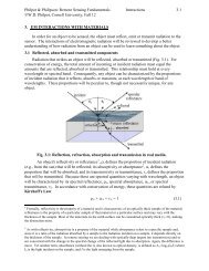
Example<br />
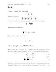
Consider a bar of length L, cross-sectional area A which is held<br />
fixed on <strong>the</strong> left end and pulled with a force F on <strong>the</strong> right end and<br />
stretched with a distributed force b(x) along its length. Whats will<br />
be <strong>the</strong> deformation of <strong>the</strong> bar u(x) at each point x?<br />
b(x)<br />
A<br />
u(x)<br />
L<br />
F<br />
Boundary Value Problem (BVP)<br />
EA d 2 u(x)<br />
dx 2 + b(x) = 0 ∀x ∈ (0, L) (1)<br />
with boundary conditions: u(0) = 0,<br />
E A du<br />
dx | x=l = F
Boundary Value Problem<br />
<strong>Lecture</strong> <strong>02</strong><br />
pk285@<br />
Boundary<br />
Value<br />
Problems<br />
<strong>Finite</strong> <strong>Element</strong><br />
<strong>Method</strong><br />
Function Spaces<br />
Weak Forms<br />
Boundary Value Problem (BVP)<br />
EA d 2 u(x)<br />
dx 2 + b(x) = 0 ∀x ∈ (0, L) (2)<br />
with boundary conditions: u(0) = 0, E A du<br />
dx | x=l = F<br />
Although it is straightforward <strong>to</strong> derive a closed-form<br />
solution (right?) things are not necessarily so if:<br />
elastic modulus varies E(x)<br />
cross-sectional area varies A(x)<br />
if we are considering two or three dimensional versions<br />
with arbitrary boundary shapes/conditions.<br />
we need a general computational method that is able <strong>to</strong><br />
produce efficiently, accurate solutions of BVPs.
Boundary Value Problem<br />
<strong>Lecture</strong> <strong>02</strong><br />
pk285@<br />
Boundary<br />
Value<br />
Problems<br />
<strong>Finite</strong> <strong>Element</strong><br />
<strong>Method</strong><br />
Function Spaces<br />
Weak Forms<br />
Boundary Value Problem (BVP)<br />
EA d 2 u(x)<br />
dx 2 + b(x) = 0 ∀x ∈ (0, L) (3)<br />
Approximate derivatives with finite differences, i.e.:<br />
du<br />
dx = lim u(x + h) − u(x) u(x + h) − u(x)<br />
≈ for 0 < h
Boundary Value Problem<br />
<strong>Lecture</strong> <strong>02</strong><br />
pk285@<br />
Boundary<br />
Value<br />
Problems<br />
<strong>Finite</strong> <strong>Element</strong><br />
<strong>Method</strong><br />
Function Spaces<br />
Weak Forms<br />
Boundary Value Problem (BVP)<br />
EA d 2 u(x)<br />
dx 2 + b(x) = 0 ∀x ∈ (0, L) (4)<br />
define N grid points x i = i h where h = L N<br />
and let<br />
u i = u(x i )<br />
if h is small enough <strong>the</strong>n I can approximate:<br />
d 2 u(x)<br />
dx 2 | x=xi ≈ u i+1 − 2u i + u i−1<br />
h 2 (5)<br />
substitute in Equation (4) for x = x i , ∀i <strong>to</strong> obtain N<br />
algebraic equations w.r.t N unknowns u i .<br />
this is <strong>the</strong> <strong>the</strong> <strong>Finite</strong> Difference <strong>Method</strong>
<strong>Finite</strong> Difference <strong>Method</strong> (FDM)<br />
<strong>Lecture</strong> <strong>02</strong><br />
pk285@<br />
Boundary<br />
Value<br />
Problems<br />
<strong>Finite</strong> <strong>Element</strong><br />
<strong>Method</strong><br />
Function Spaces<br />
Weak Forms<br />
E d 2 u(x)<br />
dx 2 + b(x) = 0 ∀x ∈ (0, L)<br />
⇓<br />
(discretization)<br />
EA u i+1 − 2u i + u i−1<br />
h 2 + b(x i ) = 0 ∀x i , i = 1, 2,...,N<br />
Observe that in FDM we approximate <strong>the</strong> PDE itself<br />
FDM is still used in a wide range of problems and we<br />
will use it in time-dependent problems <strong>to</strong> discretize<br />
time derivatives.<br />
In <strong>the</strong> <strong>Finite</strong> <strong>Element</strong> <strong>Method</strong> (FEM) we approximate<br />
<strong>the</strong> solution of <strong>the</strong> PDE.
<strong>Finite</strong> <strong>Element</strong> <strong>Method</strong><br />
<strong>Lecture</strong> <strong>02</strong><br />
pk285@<br />
Boundary<br />
Value<br />
Problems<br />
<strong>Finite</strong> <strong>Element</strong><br />
<strong>Method</strong><br />
Function Spaces<br />
Weak Forms<br />
Roadmap <strong>to</strong> FEM approximations:<br />
1 We are going <strong>to</strong> define where we are going <strong>to</strong> <strong>to</strong> be looking<br />
for solutions, i.e. which function space<br />
2 We are going <strong>to</strong> reformulate <strong>the</strong> original problem, i.e. PDE<br />
and BC.<br />
3 We are going <strong>to</strong> show that this new form is actually<br />
equivalent <strong>to</strong> <strong>the</strong> original, i.e. any solution of <strong>the</strong> former is a<br />
solution of <strong>the</strong> latter and vice versa.<br />
4 We are going <strong>to</strong> show that <strong>the</strong> solution is unique.<br />
5 If that wasn’t enough, we are going <strong>to</strong> look at some<br />
equivalent forms which can be considered as special cases.<br />
6 We are going <strong>to</strong> propose ways <strong>to</strong> discretize <strong>the</strong>se alternate<br />
forms.
Function Spaces<br />
<strong>Lecture</strong> <strong>02</strong><br />
pk285@<br />
Boundary<br />
Value<br />
Problems<br />
<strong>Finite</strong> <strong>Element</strong><br />
<strong>Method</strong><br />
Function Spaces<br />
Weak Forms<br />
Since we are going <strong>to</strong> be approximating solutions of PDEs<br />
i.e. functions, it makes sense <strong>to</strong> recap some of <strong>the</strong> basic<br />
function spaces and <strong>the</strong>ir properties. If Ω is an open subset<br />
of R (or R n ) in general, <strong>the</strong>n:<br />
C(Ω) contains all functions defined on Ω which are<br />
continuous.<br />
C k (Ω) contains all functions defined on Ω which have<br />
continuous derivatives up <strong>to</strong> order k.<br />
Cb k(Ω) same as Ck (Ω) plus <strong>the</strong> function is bounded<br />
L 2 (Ω) contains all functions defined on Ω which are square<br />
integrable i.e.: ∫<br />
u 2 (x) dx < +∞ (6)<br />
Ω<br />
H 1 (Ω) contains all functions in L 2 whose derivatives are also<br />
square integrable i.e.:<br />
∫<br />
|du/dx| 2 (x) dx < +∞ (7)<br />
Ω
Function Spaces<br />
<strong>Lecture</strong> <strong>02</strong><br />
pk285@<br />
Boundary<br />
Value<br />
Problems<br />
<strong>Finite</strong> <strong>Element</strong><br />
<strong>Method</strong><br />
Function Spaces<br />
Weak Forms<br />
Boundary Value Problem (BVP)<br />
EA d 2 u(x)<br />
dx 2 + b(x) = 0 ∀x ∈ (0, L) (8)<br />
with boundary conditions: u(0) = u 0 ,<br />
E A du<br />
dx | x=l = F<br />
We are going <strong>to</strong> look for solutions in <strong>the</strong> space S:<br />
∫<br />
S = {u(x) : (0, L) → R|u(0) = u 0 , E A| du<br />
dx |2 (x) dx < +∞}<br />
(0,L)<br />
Observe that:<br />
u ∈ S satisfy exactly only one of <strong>the</strong> two boundary<br />
conditions. This BC is called essential.<br />
u ∈ S have finite strain energy!<br />
u ∈ S are continuous and bounded.
Function Spaces<br />
<strong>Lecture</strong> <strong>02</strong><br />
pk285@<br />
Boundary<br />
Value<br />
Problems<br />
<strong>Finite</strong> <strong>Element</strong><br />
<strong>Method</strong><br />
Function Spaces<br />
Weak Forms<br />
Boundary Value Problem (BVP)<br />
EA d 2 u(x)<br />
dx 2 + b(x) = 0 ∀x ∈ (0, L) (9)<br />
with boundary conditions: u(0) = u 0 , E A du<br />
dx | x=l = F<br />
We are going <strong>to</strong> look for solutions in <strong>the</strong> space S:<br />
∫<br />
S = {u(x) : (0, L) → R|u(0) = u 0 ,<br />
(0,L)<br />
E A| du<br />
dx |2 (x) dx < +∞}<br />
Observe that:<br />
The space S is much larger than what <strong>the</strong> PDE and BC<br />
would imply.<br />
Even though a 2nd order derivative of appears in<br />
Equation (9), we are looking for solutions that are<br />
guaranteed <strong>to</strong> have a 1st order derivative<br />
Even though a “force” BC must be satisfied, we are<br />
looking for solutions that are not a priori guaranteed <strong>to</strong><br />
satisfy it.
<strong>Finite</strong> <strong>Element</strong> <strong>Method</strong><br />
<strong>Lecture</strong> <strong>02</strong><br />
pk285@<br />
Boundary<br />
Value<br />
Problems<br />
<strong>Finite</strong> <strong>Element</strong><br />
<strong>Method</strong><br />
Function Spaces<br />
Weak Forms<br />
Roadmap <strong>to</strong> FEM approximations:<br />
1 We are going <strong>to</strong> define where we are going <strong>to</strong> <strong>to</strong> be looking<br />
for solutions, i.e. which function space<br />
2 We are going <strong>to</strong> reformulate <strong>the</strong> original problem, i.e. PDE<br />
and BC.<br />
3 We are going <strong>to</strong> show that this new form is actually<br />
equivalent <strong>to</strong> <strong>the</strong> original, i.e. any solution of <strong>the</strong> former is a<br />
solution of <strong>the</strong> latter and vice versa.<br />
4 We are going <strong>to</strong> show that <strong>the</strong> solution is unique.<br />
5 If that wasn’t enough, we are going <strong>to</strong> look at some<br />
equivalent forms which can be considered as special cases.<br />
6 We are going <strong>to</strong> propose ways <strong>to</strong> discretize <strong>the</strong>se alternate<br />
forms.
Weak Forms<br />
<strong>Lecture</strong> <strong>02</strong><br />
pk285@<br />
Boundary<br />
Value<br />
Problems<br />
<strong>Finite</strong> <strong>Element</strong><br />
<strong>Method</strong><br />
Function Spaces<br />
Weak Forms<br />
Boundary Value Problem (BVP)<br />
EA d 2 u(x)<br />
dx 2 + b(x) = 0 ∀x ∈ (0, L) (10)<br />
with boundary conditions: u(0) = u 0 , E A du<br />
dx | x=l = F<br />
We are going <strong>to</strong> look for solutions in <strong>the</strong> space S:<br />
∫<br />
S = {u(x) : (0, L) → R|u(0) = u 0 ,<br />
(0,L)<br />
E A| du<br />
dx |2 (x) dx < +∞}<br />
A u ∈ S will not satisfy Equation (10) exactly (unless it is <strong>the</strong><br />
solution) and in general <strong>the</strong>re will be a residual R(x)<br />
R(x) = EA d 2 u(x)<br />
dx 2 + b(x) (11)<br />
There will also be a residual R(L) = E A du<br />
dx | x=l − F because<br />
u ∈ S do not a priori satisfy this BC
Weak Forms<br />
<strong>Lecture</strong> <strong>02</strong><br />
pk285@<br />
Boundary<br />
Value<br />
Problems<br />
<strong>Finite</strong> <strong>Element</strong><br />
<strong>Method</strong><br />
Function Spaces<br />
Weak Forms<br />
How can we make those residuals zero?<br />
R(x) = EA d 2 u(x)<br />
dx 2 + b(x) R(L) = F − EA du<br />
dx | x=l<br />
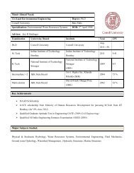
(Bubnov)-Galerkin approach<br />
Figure: Boris Galerkin (1871-1945)
Weak Forms<br />
<strong>Lecture</strong> <strong>02</strong><br />
pk285@<br />
Boundary<br />
Value<br />
Problems<br />
<strong>Finite</strong> <strong>Element</strong><br />
<strong>Method</strong><br />
Function Spaces<br />
Weak Forms<br />
How can we make those residuals zero?<br />
R(x) = EA d 2 u(x)<br />
dx 2 + b(x) R(L) = F − EA du<br />
dx | x=l<br />
(Bubnov)-Galerkin or Weighted Residual approach: define<br />
ano<strong>the</strong>r set of functions called weighting functions v ∈ V:<br />
∫<br />
V = {v(x) : (0, L) → R|v(0) = 0, E A| dv<br />
dx |2 (x) dx < +∞}<br />
(0,L)<br />
Find u ∈ S such that for all v ∈ V:<br />
∫ L<br />
0<br />
v(x)R(x) dx + v(L)R(L) = 0 (12)<br />
Note that <strong>the</strong> residual is not zero in <strong>the</strong> STRONG sense i.e.<br />
R(x) = 0 ∀x but <strong>the</strong> condition is enforced WEAKLY as above.
Weak Forms<br />
<strong>Lecture</strong> <strong>02</strong><br />
pk285@<br />
Boundary<br />
Value<br />
Problems<br />
<strong>Finite</strong> <strong>Element</strong><br />
<strong>Method</strong><br />
Function Spaces<br />
Weak Forms<br />
STRONG form:<br />
WEAK form:<br />
⎧ ∫ L<br />
⎨<br />
0<br />
u ∈ S<br />
⎩<br />
v ∈ V<br />
du dv<br />
EA<br />
dx<br />
⎧<br />
⎨<br />
⎩<br />
EA d 2 u(x)<br />
dx 2 + b(x) = 0<br />
u(0) = u 0<br />
F = EA du<br />
dx | x=l<br />
dx dx = ∫ L<br />
A b(x)v(x)dx + v(L)F ∀v ∈ V<br />
0<br />
Does <strong>the</strong> weak form remind you of something?<br />
Principle of Virtual Work<br />
The necessary and sufficient condition for a system in<br />
equilibrium is that <strong>the</strong> work done by internal forces should be<br />
equal <strong>to</strong> <strong>the</strong> work done by externals loads for any<br />
kinematically acceptable virtual displacement
Weak Forms<br />
<strong>Lecture</strong> <strong>02</strong><br />
pk285@<br />
Boundary<br />
Value<br />
Problems<br />
<strong>Finite</strong> <strong>Element</strong><br />
<strong>Method</strong><br />
Function Spaces<br />
Weak Forms<br />
WEAK form:<br />
⎧ ∫ L<br />
⎨<br />
0<br />
u ∈ S<br />
⎩<br />
v ∈ V<br />
du dv<br />
EA<br />
dx<br />
Principle of Virtual Work:<br />
dx dx = ∫ L<br />
A b(x)v(x)dx + v(L) F ∀v ∈ V<br />
0<br />
a virtual kinematically acceptable displacement v(x) is<br />
one that does not violate displacement boundary<br />
conditions u(0) = u 0 , i.e. v(0) = 0.<br />
Work of internal forces:<br />
∫<br />
W int (v) = A<br />
σ u (x)<br />
} {{ }<br />
stress from u<br />
∫<br />
ǫ v (x) dx = A<br />
} {{ }<br />
strain from v<br />
Work of external forces:<br />
∫<br />
W ext (v) = A b(x) v(x) dx + F v(l)<br />
E du<br />
dx<br />
dv<br />
dx dx