Discrete probability measures Uniform measure Random variables ...
Discrete probability measures Uniform measure Random variables ...
Discrete probability measures Uniform measure Random variables ...

You also want an ePaper? Increase the reach of your titles
YUMPU automatically turns print PDFs into web optimized ePapers that Google loves.
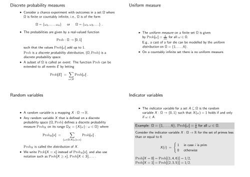
<strong>Discrete</strong> <strong>probability</strong> <strong><strong>measure</strong>s</strong><br />
◮ Consider a chance experiment with outcomes in a set Ω where<br />
Ω is finite or countably infinite, i.e., Ω is of the form<br />
<strong>Uniform</strong> <strong>measure</strong><br />
Ω = {ω 1 , . . . , ω n } or Ω = {ω 1 , ω 2 , . . .} .<br />
◮ The probabilities are given by a real-valued function<br />
Prob : Ω → [0, 1]<br />
such that the values Prob[ω] add up to 1.<br />
Prob is a discrete <strong>probability</strong> distribution, (Ω, Prob) is a<br />
discrete <strong>probability</strong> space.<br />
◮ A subset of Ω is called an event. The function Prob can be<br />
extended to all events E by letting<br />
◮ The uniform <strong>measure</strong> on a finite set Ω is given<br />
by Prob[ω] = 1<br />
|Ω|<br />
for all ω ∈ Ω.<br />
E.g., a cast of a fair die can be modelled by the uniform<br />
distribution on Ω = {1, . . . , 6}.<br />
◮ On a countably infinite set there is no uniform <strong>measure</strong>.<br />
Prob[E] = ∑ ω∈E<br />
Prob[ω] .<br />
<strong>Random</strong> <strong>variables</strong><br />
Indicator <strong>variables</strong><br />
◮ A random variable is a mapping X : Ω → R.<br />
◮ Any random variable X that is defined on a discrete<br />
<strong>probability</strong> space (Ω, Prob) defines a discrete <strong>probability</strong><br />
<strong>measure</strong> Prob X on its range Ω X = {X (ω) : ω ∈ Ω} where<br />
Prob X [x] =<br />
∑<br />
{ω∈Ω:X (ω)=x}<br />
Prob X is called the distribution of X .<br />
Prob[ω] .<br />
◮ We write Prob[X = x] instead of Prob X [x], and also use<br />
notation such as Prob[X ≥ x], Prob[X ∈ S], . . . .<br />
◮ The indicator variable for a set A ⊆ Ω is the random<br />
variable X : Ω → {0, 1} such that X (ω) = 1 holds if and only<br />
if ω ∈ A.<br />
Example: Ω = {1, . . . , 6}, Prob[ω] = 1 6<br />
for all ω ∈ Ω.<br />
Consider the indicator variable X : Ω → R for the set of primes less<br />
than or equal to 6<br />
{<br />
1 in case i is prim<br />
X (i) =<br />
0 otherwise<br />
Prob[X = 0] = Prob[{1, 4, 6}] = 1/2,<br />
Prob[X = 1] = Prob[{2, 3, 5}] = 1/2.
Joint distribution<br />
Joint distribution<br />
◮ Let X 1 , . . . , X m be random <strong>variables</strong> on the same discrete<br />
<strong>probability</strong> space Ω.<br />
◮ The joint distribution Prob X1 ,...,X m<br />
Prob X1 ,...,X m<br />
[r 1 , . . . , r m ] =<br />
is<br />
∑<br />
{ω∈Ω:X 1 (ω)=r 1 ,...,X m (ω)=r m }<br />
◮ We write Prob[X 1 = r 1 , . . . , X m = r m ] instead<br />
of Prob X1 ,...,X m<br />
[r 1 , . . . , r m ].<br />
Prob[ω] . (1)<br />
Example: Ω = {1, . . . , 6}, Prob[ω] = 1 6<br />
for all ω ∈ Ω.<br />
Consider indicator <strong>variables</strong> X , Y and Z for the events ω is prime,<br />
ω is even, and ω is odd.<br />
X , Y , and Z have the same distribution, the uniform distribution<br />
on {0, 1}. However,<br />
Prob[X = 1, Y = 1] = 1 6 ,<br />
Prob[X = 1, Z = 1] = 2 6 .<br />
So the joint distribution is not determined by the individual<br />
distributions.<br />
Mutually independent random <strong>variables</strong><br />
◮ Let X 1 , . . . , X m be random <strong>variables</strong> on the same discrete<br />
<strong>probability</strong> space Ω.<br />
◮ X 1 , . . . , X m are mutually independent if for any combination<br />
of values r 1 , . . . , r m in the range of X 1 , . . . , X m , respectively,<br />
Prob[X 1 = r 1 , . . . , X m = r m ]<br />
Example: m tosses of a fair coin<br />
= Prob[X 1 = r 1 ] · · · · · Prob[X m = r m ] .<br />
Consider m tosses of a fair coin and let X i be the indicator variable<br />
for the event that the ith toss shows head. Then the X 1 , . . . , X m<br />
are mutually independent and for all (r 1 . . . r m ) ∈ {0, 1} m<br />
Prob[X 1 = r 1 , . . . , X m = r m ] = 1<br />
2 m .<br />
Pairwise and k-wise independence<br />
◮ <strong>Random</strong> <strong>variables</strong> X 1 , . . . , X m are pairwise independent if all<br />
pairs X i and X j with i ≠ j are mutually independent, i.e., for<br />
all i ≠ j and all r i and r j<br />
Prob[X i = r i and X j = r j ]<br />
= Prob[X i = r i ] · Prob[X j = r j ] .<br />
◮ The concept of k-wise independence of random <strong>variables</strong> for<br />
any k ≥ 2 is defined similar to pairwise independence, where<br />
now every subset of k distinct random <strong>variables</strong> must be<br />
mutually independent.
Mutual versus pairwise independence<br />
Pairwise and 3-wise independence<br />
◮ It can be shown that mutual independence implies pairwise<br />
independence.<br />
◮ For three or more random <strong>variables</strong>, in general pairwise<br />
independence does not imply mutual independence.<br />
◮ It can be shown for any k ≥ 2 that (k + 1)-wise independence<br />
implies k-wise independence, whereas the reverse implication<br />
is false.<br />
◮ Examples of random <strong>variables</strong> that are k-wise independent but<br />
are not mutually independent will be constructed in the<br />
section on derandomization.<br />
An even simpler example is the following.<br />
Example: pairwise but not 3-wise independence.<br />
Consider a chance experiment where a fair coin is tossed 3 times<br />
and let X i be the indicator variable for the event that coin i shows<br />
head. Let<br />
Z 1 = X 1 ⊕ X 2 , Z 2 = X 1 ⊕ X 3 , Z 3 = X 2 ⊕ X 3 .<br />
The random <strong>variables</strong> Z 1 , Z 2 , and Z 3 are pairwise independent<br />
because for any pair i and j of distinct indices in {1, 2, 3} and any<br />
values b 1 and b 2 in {0, 1} we have<br />
Prob[Z i = b 1 &Z j = b 2 ] = 1/4 .<br />
On the other hand, Z 1 , Z 2 , and Z 3 are not 3-wise independent<br />
because for example we have Z 1 = Z 2 ⊕ Z 3 .<br />
Expectation<br />
◮ The expectation of X is<br />
Expectation<br />
Example: Ω = {1, . . . , 6}, Prob[ω] = 1 6<br />
for all ω ∈ Ω.<br />
E [X ] = ∑ ω∈Ω<br />
Prob[ω]X (ω) ,<br />
provided that this sum converges absolutely. If the latter<br />
condition is satisfied, we say the expectation of X exists.<br />
◮ Recall ∑ that<br />
◮<br />
i∈N a i converges to s if and only if the partial<br />
∑<br />
sums a 0 + . . . + a n converge to s,<br />
◮<br />
i∈N a i converges absolutely if even the sum ∑ i∈N |a i|<br />
converges,<br />
◮ absolute convergence is equivalent to convergence to the same<br />
value under arbitrary reorderings.<br />
◮ The condition on absolute convergence ensures that the<br />
expectation is the same no matter how we order Ω.<br />
The condition is always satisfied if Ω is finite or if X is<br />
non-negative and the sum converges at all.<br />
If we let X be the identity mapping on Ω, then<br />
E [X ] =<br />
∑<br />
i∈{1,...,6}<br />
Example: Ω = N, Prob[i] = 1<br />
2 i+1 .<br />
Prob[i] X (i) = 1 6 + 2 6 + . . . + 6 6 = 21 6 = 3.5 .<br />
The expectation of the random variable<br />
X : i ↦→ 2 i+1<br />
does not exist because the corresponding sum does not converge<br />
∑<br />
i∈N<br />
Prob[i] X (i) = ∑ i∈N<br />
1<br />
2 i+1 2i+1 = 1 + 1 + . . . = +∞ .
Linearity of Expectation<br />
◮ Let X and X 1 , . . . , X n be random <strong>variables</strong> such that their<br />
expectations all exist.<br />
◮ Expectation is linear.<br />
For any real number r, the expectation of rX exists and it<br />
holds that<br />
E [rX ] = rE [X ] .<br />
The expectation of X 1 + . . . + X m exists and it holds that<br />
E [X 1 + · · · + X n ] = E [X 1 ] + · · · + E [X n ] .<br />
◮ If the X 1 , . . . , X n are mutually independent, then the<br />
expectation of X 1 · . . . · X m exists and<br />
E [X 1 · · · · · X n ] = E [X 1 ] · · · · · E [X n ] .<br />
Number of fixed points of a random permutation<br />
◮ Suppose that n tokens T 1 , . . . , T n are distributed at random<br />
among n persons P 1 , . . . , P n such that each person gets<br />
exactly one token and all such assignments of tokens to<br />
persons have the same <strong>probability</strong><br />
(i.e., the tokens are assigned by choosing a permutation<br />
of {1, . . . , n} uniformly at random).<br />
◮ What is the expected number of indices i such that P i gets<br />
his or her “own token” T i ?<br />
If we let X i be the indicator variable for the event that P i<br />
gets T i , then X = ∑ n<br />
i=1 X i is equal to the random number of<br />
persons that get their own token.<br />
◮ By linearity of expectation, the expectation of X is<br />
[ n∑<br />
]<br />
n∑<br />
n∑<br />
( n − 1<br />
E [X ] = E X i = E [X i ] =<br />
n 0 + 1 )<br />
n 1 = 1 .<br />
i=1<br />
i=1<br />
i=1<br />
Conditional distributions and expectations<br />
◮ The conditional <strong>probability</strong> of an event E given an event F is<br />
Prob[E|F ] = Prob[E ∩ F ]<br />
Prob[F ]<br />
where this value is undefined in case Prob[F ] = 0.<br />
◮ The conditional distribution Prob[.|F ] of a random variable X<br />
given an event F is defined by<br />
Prob[X = a|F ] =<br />
Prob[{ω ∈ Ω: X (ω) = a} ∩ F ]<br />
Prob[F ]<br />
◮ The conditional expectation E [X |F ] of a random variable X<br />
given an event F is the expectation of X with respect to the<br />
conditional distribution Prob[X |F ], i.e.,<br />
∑<br />
E [X |F ] = a · Prob[X = a|F ] .<br />
a∈range(X )<br />
,<br />
.<br />
Markov Inequality<br />
Proposition (Markov Inequality)<br />
Let X be a random variable that assumes only non-negative values.<br />
Then for every positive real number r, we have<br />
Proof.<br />
Prob[X ≥ r] ≤ E [X ]<br />
r<br />
Let (Ω, Prob) be the <strong>probability</strong> space on which X is defined.<br />
Then we have<br />
E [X ] = ∑ ∑<br />
Prob[ω]X (ω) ≥<br />
Prob[ω]X (ω)<br />
ω∈Ω<br />
≥<br />
r<br />
∑<br />
{ω∈Ω:X (ω)≥r}<br />
.<br />
{ω∈Ω:X (ω)≥r}<br />
Prob[ω] ≥ r Prob[X ≥ r] .