Journal of AE, Volume 27, 2009 (ca. 35 MB) - AEWG
Journal of AE, Volume 27, 2009 (ca. 35 MB) - AEWG
Journal of AE, Volume 27, 2009 (ca. 35 MB) - AEWG

You also want an ePaper? Increase the reach of your titles
YUMPU automatically turns print PDFs into web optimized ePapers that Google loves.
<strong>Journal</strong> <strong>of</strong> Acoustic Emission, <strong>Volume</strong> <strong>27</strong>, <strong>2009</strong><br />
VIEWING AN ARTICLE IN CD-ROM<br />
You need a s<strong>of</strong>tware that <strong>ca</strong>n read a pdf-file, such as Adobe Acrobat Reader®. Install one first before<br />
going further. You <strong>ca</strong>n download the latest version from www.adobe.com. Use <strong>of</strong> Adobe Acrobat® (not<br />
provided) allows one to utilize the Search function. This gives the power to search for a name or a word<br />
in the entire volume and is highly recommended.<br />
PDF Files: Contents are listed below. Individual papers have file names <strong>of</strong> <strong>27</strong>-xxx.pdf, with xxx as their<br />
first page number.<br />
Contents<br />
<strong>27</strong>-001 MONITORING THE CIVIL INFRASTRUCTURE WITH ACOUSTIC EMISSION:<br />
BRIDGE CASE STUDIES<br />
D. ROBERT HAY, JOSE A. CAVACO and VASILE MUSTAFA 1-10<br />
<strong>27</strong>-011 ACOUSTIC EMISSION TESTING OF A DIFFICULT-TO-REACH STEEL BRIDGE<br />
DETAIL<br />
DAVID E. KOSNIK 11-17<br />
<strong>27</strong>-018 ACOUSTIC EMISSION AS A MONITORING METHOD IN PRESTRESSED<br />
CONCRETE BRIDGES HEALTH CONDITION EVALUATION<br />
MAŁGORZATA KALICKA 18-26<br />
<strong>27</strong>-0<strong>27</strong> ACOUSTIC EMISSION LEAK DETECTION OF LIQUID FILLED<br />
BURIED PIPELINE<br />
ATHANASIOS ANASTASOPOULOS, DIMITRIOS KOUROUSIS<br />
and KONSTANTINOS BOLLAS <strong>27</strong>-39<br />
<strong>27</strong>-040 ACOUSTIC EMISSION MONITORING AND FATIGUE LIFE<br />
PREDICTION IN AXIALLY LOADED NOTCHED STEEL SPECIMENS<br />
FADY F. BARSOUM, JAMIL SULEMAN, ANDREJ KORCAK and ERIC V. K. HILL 40-63<br />
<strong>27</strong>-064 <strong>AE</strong> ANALYSIS ON BLADE CUTTING PRESSURE ADJUSTMENT IN DYNAMIC<br />
CUTTING OF PAPERBOARD<br />
DARULIHSAN A. HAMID, SHIGERU NAGASAWA, YASUSHI FUKUZAWA,<br />
YUUKI KOMIYAMA and AKIRA HINE 64-76<br />
<strong>27</strong>-077 DAMAGE ONSET AND GROWTH IN CARBON-CARBON COMPOSITE<br />
MONITORED BY ACOUSTIC EMISSION TECHNIQUE<br />
ARIE BUSSIBA, ROMANA PIAT, MOSHE KUPIEC, RAMI CARMI, IGAL ALON<br />
and THOMAS BÖHLKE 77-88<br />
<strong>27</strong>-089 FUNDAMENTAL STUDY ON INTEGRITY EVALUATION METHOD FOR COPVS<br />
BY MEANS OF ACOUSTIC EMISSION TESTING<br />
YOSHIHIRO MIZUTANI, SOTA SUGIMOTO, RYOSUKE MATSUZAKI<br />
and AKIRA TODOROKI 89-97<br />
I-1
<strong>27</strong>-098 ACOUSTIC EMISSION FROM IMPACTS OF RIGID BODIES<br />
TATIANA B. PETERSEN 98-113<br />
<strong>27</strong>-114 SOME OBSERVATIONS ON RAYLEIGH WAVES AND ACOUSTIC EMISSION IN<br />
THICK STEEL PLATES<br />
M. A. HAMSTAD 114-136<br />
<strong>27</strong>-137 FRACTURE BEHAVIOR IN BONE CHARACTERIZED BY <strong>AE</strong> WAVELET<br />
ANALYSIS<br />
SHUICHI WAKAYAMA, KEISUKE MOGI and TETSUYA SUEMUNE 137-143<br />
<strong>27</strong>-144 ABOUT PLASTIC INSTABILITIES IN IRON AND POWER SPECTRUM OF<br />
ACOUSTIC EMISSION<br />
ALEXEY LAZAREV and ALEXEI VINOGRADOV 144-156<br />
<strong>27</strong>-157 ACOUSTIC AND ELECTROMAGNETIC EMISSION FROM CRACK<br />
CREATED IN ROCK SAMPLE UNDER DEFORMATION<br />
YASUHIKO MORI, YOSHIHIKO OBATA and JOSEF SIKULA 157-166<br />
<strong>27</strong>-167 IDENTIFICATION OF <strong>AE</strong> MULTIPLETS IN THE TIME AND FREQUENCY<br />
DOMAINS<br />
HIROSHI ASANUMA, YUSUKE KUMANO, HIROAKI NIITSUMA, DOONE WYBORN<br />
and ULRICH SCANZ 167-175<br />
<strong>27</strong>-176 CRACK GROWTH MONITORING WITH HIERARCHICAL CLUSTERING OF <strong>AE</strong><br />
N. F. INCE, CHU-SHU KAO, M. KAVEH, A. TEWFIK and J. F. LABUZ 176-185<br />
<strong>27</strong>-186 ACOUSTIC EMISSION FOR CHARACTERIZING BEHAVIOR OF COMPOSITE<br />
CONCRETE ELEMENTS UNDER FLEXURE<br />
SHOHEI MOMOKI, HWAKIAN CHAI, DIMITRIOS G. AGGELIS, AKINOBU HIRAMA<br />
and TOMOKI SHIOTANI 186-193<br />
<strong>27</strong>-194 DISTINCT ELEMENT ANALYSIS FOR ROCK FAILURE CONSIDERING <strong>AE</strong><br />
EVENTS GENERATED BY THE SLIP AT CRACK SURFACES<br />
HIROYUKI SHIMIZU, SUMIHIKO MURATA and TSUYOSHI ISHIDA 194-211<br />
<strong>27</strong>-212 ELECTROMAGNETIC METHOD OF ELASTIC WAVE EXCITATION FOR<br />
CALIBRATION OF ACOUSTIC EMISSION SENSORS AND APPARATUS<br />
SERGEY LAZAREV, ALEXANDER MOZGOVOI, ALEXEI VINOGRADOV, ALEXEY LAZAREV<br />
and ANDREY SHVEDOV 212-223<br />
<strong>27</strong>-224 MONITORING OF PIPE CLOGGING BY MUSSELS UTILIZING AN OPTICAL<br />
FIBER <strong>AE</strong> SYSTEM<br />
TAKUMA MATSUO, YUTA MIZUNO and HIDEO CHO 224-232<br />
<strong>27</strong>-233 CORROSION DETECTION BY FIBER OPTIC <strong>AE</strong> SENSOR<br />
YUICHI MACHIJIMA, MASAHIRO AZEMOTO, TOYOKAZU TADA<br />
I-2
and HISAKAZU MORI 233-240<br />
<strong>27</strong>-241 EFFECT OF SHOT PEENING ON THE DELAYED FRACTURE USING THE<br />
ALMEN STRIP AND <strong>AE</strong> TECHNIQUE<br />
MIKIO TAKEMOTO, MOTOAKI NAKAMURA, SEIJI MASANO and SHUICHI UENO 241-253<br />
<strong>27</strong>-254 CONTRIBUTION OF ACOUSTIC EMISSION TO EVALUATE CABLE STRESS<br />
CORROSION CRACKING IN SIMULATED CONCRETE PORE SOLUTION<br />
S. RAMADAN, L. GAILLET, C. TESSIER and H. IDRISSI 254-262<br />
<strong>27</strong>-263 FLEXURAL FAILURE BEHAVIOR OF RC BEAMS WITH REBAR CORROSION<br />
AND DAMAGE EVALUATION BY ACOUSTIC EMMISSION<br />
NOBUHIRO OKUDE, MINORU KUNIEDA, TOMOKI SHIOTANI<br />
and HIKARU NAKAMURA 263-<strong>27</strong>1<br />
<strong>27</strong>-<strong>27</strong>2 ACOUSTIC EMISSION METHOD FOR SOLVING PROBLEMS IN DOUBLE-<br />
BOTTOM STORAGE TANKS<br />
MAREK NOWAK, IRENEUSZ BARAN, JERZY SCHMIDT and KANJI ONO <strong>27</strong>2-280<br />
<strong>27</strong>-281 STUDY OF IDENTIFICATION AND REMOVAL METHOD FOR DROP NOISE IN<br />
<strong>AE</strong> MEASUREMENT OF TANKS<br />
HIDEYUKI NAKAMURA, TAKAHIRO ARAKAWA, HIRAKU KAWASAKI, KAZUYOSHI<br />
SEKINE and NAOYA KASAI 281-290<br />
<strong>27</strong>-291 A GENERIC TECHNIQUE FOR ACOUSTIC EMISSION SOURCE LOCATION<br />
JONATHAN J. SCHOLEY, PAUL D. WILCOX, MICH<strong>AE</strong>L R. WISNOM,<br />
MIKE I. FRISWELL, MARTYN PAVIER and MOHAMMAD R ALIHA 291-298<br />
<strong>27</strong>-299 ACOUSTIC EMISSION TESTING – DEFINING A NEW STANDARD OF<br />
ACOUSTIC EMISSION TESTING FOR PRESSURE VESSELS<br />
Part 1: Quantitative and comparative performance analysis <strong>of</strong> zonal lo<strong>ca</strong>tion and<br />
triangulation methods<br />
JOHANN CATTY 299-313<br />
Contents<strong>27</strong> Contents <strong>of</strong> <strong>Volume</strong> <strong>27</strong> (<strong>2009</strong>) I-1 – I-3<br />
AUindex<strong>27</strong> Authors Index <strong>of</strong> <strong>Volume</strong> <strong>27</strong> I-4<br />
AusNotes Policy/Author’s Notes/Meeting Calendar/DVD/Subscription Information<br />
I-5 – I-7<br />
I<strong>AE</strong>S19 JC<strong>AE</strong> Kishinoue Award Acceptace Speech by T.F. Drouillard I-8 – I-10<br />
<strong>AE</strong> Literature <strong>AE</strong> conference proceedings in China, 2001-2006: Gongtian Shen I-11 – I-16<br />
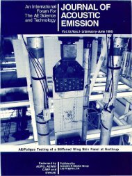
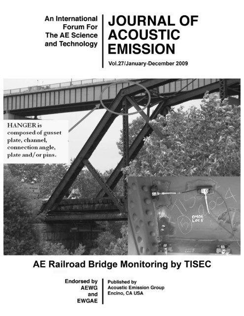
Cover photographs See <strong>27</strong>-001 by Hay et al. for details.<br />
J<strong>AE</strong> Index Folder* Cumulative Indices <strong>of</strong> J. <strong>of</strong> Acoustic Emission, 1982 – <strong>2009</strong><br />
Contents1-<strong>27</strong> Contents <strong>Volume</strong>s 1-<strong>27</strong><br />
Authors Index1-<strong>27</strong> Authors Index <strong>Volume</strong>s 1-<strong>27</strong><br />
* indi<strong>ca</strong>tes the availability in CD-ROM only. Indices are also available for download from<br />
www.aewg.org.<br />
I-3
AUTHORS INDEX, <strong>Volume</strong> <strong>27</strong>, <strong>2009</strong><br />
DIMITRIOS G. AGGELIS, <strong>27</strong>-186<br />
MOHAMMAD R ALIHA <strong>27</strong>-291<br />
IGAL ALON <strong>27</strong>-077<br />
ATHANASIOS ANASTASOPOULOS, <strong>27</strong>-0<strong>27</strong><br />
TAKAHIRO ARAKAWA, <strong>27</strong>-281<br />
HIROSHI ASANUMA, <strong>27</strong>-167<br />
MASAHIRO AZEMOTO, <strong>27</strong>-233<br />
IRENEUSZ BARAN, <strong>27</strong>-<strong>27</strong>2<br />
FADY F. BARSOUM, <strong>27</strong>-040<br />
THOMAS BÖHLKE <strong>27</strong>-077<br />
KONSTANTINOS BOLLAS <strong>27</strong>-0<strong>27</strong><br />
ARIE BUSSIBA, <strong>27</strong>-077<br />
RAMI CARMI, <strong>27</strong>-077<br />
JOHANN CATTY <strong>27</strong>-299<br />
JOSE A. CAVACO <strong>27</strong>-001<br />
HWAKIAN CHAI, <strong>27</strong>-186<br />
HIDEO CHO <strong>27</strong>-224<br />
MIKE I. FRISWELL, <strong>27</strong>-291<br />
YASUSHI FUKUZAWA, <strong>27</strong>-064<br />
L. GAILLET, <strong>27</strong>-254<br />
DARULIHSAN A. HAMID, <strong>27</strong>-064<br />
M. A. HAMSTAD <strong>27</strong>-114<br />
D. ROBERT HAY, <strong>27</strong>-001<br />
ERIC V. K. HILL <strong>27</strong>-040<br />
AKIRA HINE <strong>27</strong>-064<br />
AKINOBU HIRAMA <strong>27</strong>-186<br />
H. IDRISSI <strong>27</strong>-254<br />
N. F. INCE, <strong>27</strong>-176<br />
TSUYOSHI ISHIDA <strong>27</strong>-194<br />
MAŁGORZATA KALICKA <strong>27</strong>-018<br />
CHU-SHU KAO, <strong>27</strong>-176<br />
NAOYA KASAI <strong>27</strong>-281<br />
M. KAVEH, <strong>27</strong>-176<br />
HIRAKU KAWASAKI, <strong>27</strong>-281<br />
YUUKI KOMIYAMA <strong>27</strong>-064<br />
ANDREJ KORCAK <strong>27</strong>-040<br />
DAVID E. KOSNIK, <strong>27</strong>-011<br />
DIMITRIOS KOUROUSIS <strong>27</strong>-0<strong>27</strong><br />
YUSUKE KUMANO, <strong>27</strong>-167<br />
MINORU KUNIEDA, <strong>27</strong>-263<br />
MOSHE KUPIEC, <strong>27</strong>-077<br />
J. F. LABUZ <strong>27</strong>-176<br />
ALEXEY LAZAREV <strong>27</strong>-144, <strong>27</strong>-212<br />
SERGEY LAZAREV, <strong>27</strong>-212<br />
YUICHI MACHIJIMA, <strong>27</strong>-233<br />
SEIJI MASANO <strong>27</strong>-241<br />
TAKUMA MATSUO, <strong>27</strong>-224<br />
RYOSUKE MATSUZAKI <strong>27</strong>-089<br />
YUTA MIZUNO <strong>27</strong>-224<br />
YOSHIHIRO MIZUTANI, <strong>27</strong>-089<br />
KEISUKE MOGI <strong>27</strong>-137<br />
SHOHEI MOMOKI, <strong>27</strong>-186<br />
HISAKAZU MORI <strong>27</strong>-233<br />
YASUHIKO MORI, <strong>27</strong>-157<br />
ALEXANDER MOZGOVOI, <strong>27</strong>-212<br />
SUMIHIKO MURATA <strong>27</strong>-194<br />
VASILE MUSTAFA <strong>27</strong>-001<br />
SHIGERU NAGASAWA, <strong>27</strong>-064<br />
HIDEYUKI NAKAMURA, <strong>27</strong>-281<br />
HIKARU NAKAMURA <strong>27</strong>-263<br />
MOTOAKI NAKAMURA, <strong>27</strong>-241<br />
HIROAKI NIITSUMA, <strong>27</strong>-167<br />
MAREK NOWAK, <strong>27</strong>-<strong>27</strong>2<br />
YOSHIHIKO OBATA <strong>27</strong>-157<br />
NOBUHIRO OKUDE, <strong>27</strong>-263<br />
KANJI ONO <strong>27</strong>-<strong>27</strong>2<br />
MARTYN PAVIER <strong>27</strong>-291<br />
TATIANA B. PETERSEN <strong>27</strong>-098<br />
ROMANA PIAT, <strong>27</strong>-077<br />
S. RAMADAN, <strong>27</strong>-254<br />
ULRICH SCANZ <strong>27</strong>-167<br />
JERZY SCHMIDT <strong>27</strong>-<strong>27</strong>2<br />
JONATHAN J. SCHOLEY, <strong>27</strong>-291<br />
KAZUYOSHI SEKINE <strong>27</strong>-281<br />
HIROYUKI SHIMIZU, <strong>27</strong>-194<br />
TOMOKI SHIOTANI <strong>27</strong>-186, <strong>27</strong>-263<br />
ANDREY SHVEDOV <strong>27</strong>-212<br />
JOSEF SIKULA <strong>27</strong>-157<br />
TETSUYA SUEMUNE <strong>27</strong>-137<br />
SOTA SUGIMOTO, <strong>27</strong>-089<br />
JAMIL SULEMAN, <strong>27</strong>-040<br />
TOYOKAZU TADA <strong>27</strong>-233<br />
MIKIO TAKEMOTO, <strong>27</strong>-241<br />
C. TESSIER <strong>27</strong>-254<br />
A. TEWFIK <strong>27</strong>-176<br />
AKIRA TODOROKI <strong>27</strong>-089<br />
SHUICHI UENO <strong>27</strong>-241<br />
ALEXEI VINOGRADOV <strong>27</strong>-144, <strong>27</strong>-212<br />
SHUICHI WAKAYAMA, <strong>27</strong>-137<br />
PAUL D. WILCOX, <strong>27</strong>-291<br />
MICH<strong>AE</strong>L R. WISNOM, <strong>27</strong>-291<br />
DOONE WYBORN <strong>27</strong>-167<br />
I-4
JOURNAL OF ACOUSTIC EMISSION<br />
Editor: Kanji Ono<br />
Associate Editors: A. G. Beattie, T. F. Drouillard, M. Ohtsu and W. H. Prosser<br />
1. Aims and Scope <strong>of</strong> the <strong>Journal</strong><br />
<strong>Journal</strong> <strong>of</strong> Acoustic Emission is an international journal<br />
designed to be <strong>of</strong> broad interest and use to both researcher and<br />
practitioner <strong>of</strong> acoustic emission. It will publish original contributions<br />
<strong>of</strong> all aspects <strong>of</strong> research and signifi<strong>ca</strong>nt engineering<br />
advances in the sciences and appli<strong>ca</strong>tions <strong>of</strong> acoustic emission.<br />
The journal will also publish reviews, the abstracts <strong>of</strong> papers<br />
presented at meetings, techni<strong>ca</strong>l notes, communi<strong>ca</strong>tions and<br />
summaries <strong>of</strong> reports. Current news <strong>of</strong> interest to the acoustic<br />
emission communities, announcements <strong>of</strong> future conferences and<br />
working group meetings and new products will also be included.<br />
<strong>Journal</strong> <strong>of</strong> Acoustic Emission includes the following classes<br />
<strong>of</strong> subject matters;<br />
A. Research Articles: Manuscripts should represent completed<br />
original work embodying the results <strong>of</strong> extensive investigation.<br />
These will be judged for scientific and techni<strong>ca</strong>l merit.<br />
B. Appli<strong>ca</strong>tions: Articles must present signifi<strong>ca</strong>nt advances<br />
in the engineering appli<strong>ca</strong>tions <strong>of</strong> acoustic emission. Material will<br />
be subject to reviews for adequate description <strong>of</strong> procedures,<br />
substantial database and objective interpretation.<br />
C. Techni<strong>ca</strong>l Notes and Communi<strong>ca</strong>tions: These allow publi<strong>ca</strong>tions<br />
<strong>of</strong> short items <strong>of</strong> current interest, new or improved experimental<br />
techniques and procedures, discussion <strong>of</strong> published articles<br />
and relevant appli<strong>ca</strong>tions.<br />
D. <strong>AE</strong> Program and Data Files: Original program files and<br />
data files that <strong>ca</strong>n be read by others and analyzed will be<br />
distributed in CD-ROM.<br />
Reviews, Tutorial Articles and Special Contributions will<br />
address the subjects <strong>of</strong> general interest. Nontechni<strong>ca</strong>l part will<br />
cover book reviews, signifi<strong>ca</strong>nt personal and techni<strong>ca</strong>l accomplishments,<br />
current news and new products.<br />
2. Endorsement<br />
Acoustic Emission Working Group (<strong>AE</strong>WG), European<br />
Working Group on Acoustic Emission (EWG<strong>AE</strong>), have endorsed<br />
the publi<strong>ca</strong>tion <strong>of</strong> <strong>Journal</strong> <strong>of</strong> Acoustic Emission.<br />
3. Governing Body<br />
The Editor and Associate Editors will implement the editorial<br />
policies described above. The Editorial Board will advise the editors<br />
on any major change. The Editor, Pr<strong>of</strong>essor Kanji Ono, has<br />
the general responsibility for all the matters. Associate Editors<br />
assist the review processes as lead reviewers. The members <strong>of</strong> the<br />
Editorial Board are selected for their knowledge and experience<br />
on <strong>AE</strong> and will advise and assist the editors on the publi<strong>ca</strong>tion<br />
policies and other aspects. The Board presently includes the<br />
following members:<br />
A. Anastasopoulos (Greece)<br />
F.C. Beall<br />
(USA)<br />
J. Bohse (Germany)<br />
P. Cole (UK)<br />
L. Golaski (Poland)<br />
M.A. Hamstad<br />
(USA)<br />
R. Hay (Canada)<br />
K.M. Holford<br />
(UK)<br />
O.Y. Kwon<br />
(Korea)<br />
J.C. Lenain<br />
(France)<br />
G. Manthei (Germany)<br />
P. Mazal (Czech Republic)<br />
C.R.L. Murthy<br />
(India)<br />
A.A. Pollock<br />
(USA)<br />
F. Rauscher (Austria)<br />
T. Shiotani (Japan)<br />
P. Tschliesnig (Austria)<br />
H. Vallen (Germany)<br />
M. Wevers (Belgium)<br />
B.R.A. Wood<br />
(Australia)<br />
4. Publi<strong>ca</strong>tion<br />
<strong>Journal</strong> <strong>of</strong> Acoustic Emission is published annually in CD-<br />
ROM by Acoustic Emission Group, P<strong>MB</strong> 409, 4924 Balboa Blvd,<br />
Encino, CA 91316. It may also be reached at 2121H, Engr. V,<br />
University <strong>of</strong> California, Los Angeles, California 90095-1595<br />
(USA). tel. 310-825-5233. FAX 310-206-7<strong>35</strong>3. e-mail:<br />
aegroup7@gmail.com or ono@ucla.edu<br />
5. Subscription<br />
Subscription should be sent to Acoustic Emission Group.<br />
Annual rate for 2010 is US $111.00 including CD-ROM delivery,<br />
by priority mail in the U.S. and by air for Canada and elsewhere.<br />
For additional print copy, add $40-49. Overseas orders must be<br />
paid in US currencies with a check drawn on a US bank. PayPal<br />
payment accepted. Inquire for individual (with institutional order)<br />
and bookseller discounts. See also page I-7.<br />
6. Advertisement<br />
No advertisement will be accepted, but announcements for<br />
books, training courses and future meetings on <strong>AE</strong> will be<br />
included without charge.<br />
ISSN 0730-0050 Copyright©<strong>2009</strong> Acoustic Emission Group I-5 CODEN: JACEDO All rights reserved.
Notes for Contributors<br />
1. General<br />
The <strong>Journal</strong> will publish contributions from all parts <strong>of</strong> the<br />
world and manuscripts for publi<strong>ca</strong>tion should be submitted<br />
to the Editor. Send to:<br />
Pr<strong>of</strong>essor Kanji Ono, Editor - J<strong>AE</strong><br />
Rm. 2121H, Engr. V, MSE Dept.<br />
University <strong>of</strong> California<br />
420 Westwood Plaza,<br />
Los Angeles, California 90095-1595 USA<br />
FAX (1) 818-990-1686<br />
e-mail: ono@ucla.edu<br />
Authors <strong>of</strong> any <strong>AE</strong> related publi<strong>ca</strong>tions are encouraged to<br />
send a copy to:<br />
Mr. T.F. Drouillard, Associate Editor - J<strong>AE</strong><br />
11791 Spruce Canyon Circle<br />
Golden, Colorado 80403 USA<br />
Only papers not previously published will be accepted.<br />
Authors must agree to transfer the copyright to the <strong>Journal</strong><br />
and not to publish elsewhere, the same paper submitted to<br />
and accepted by the <strong>Journal</strong>. A paper is acceptable if it is a<br />
revision <strong>of</strong> a governmental or organizational report, or if it<br />
is based on a paper published with limited distribution.<br />
Compilation <strong>of</strong> annotated data files will be accepted for<br />
inclusion in CD-ROM distribution, so that others <strong>ca</strong>n share<br />
in their analysis for research as well as training. ASCII or<br />
widely accepted data formats will be required.<br />
The language <strong>of</strong> the <strong>Journal</strong> is English. All papers should<br />
be written concisely and clearly.<br />
2. Page Charges<br />
No page charge is levied. The contents <strong>of</strong> CD-ROM will be<br />
supplied to the authors free <strong>of</strong> charge via Internet site.<br />
3. Manuscript for Review<br />
Manuscripts for review need only to be typed legibly;<br />
preferably, double-spaced on only one side <strong>of</strong> the page with<br />
wide margins. The title should be brief. An abstract <strong>of</strong> 100-<br />
200 words is needed for articles. Except for short<br />
communi<strong>ca</strong>tions, descriptive heading should be used to<br />
divide the paper into its component parts. Use the<br />
International System <strong>of</strong> Units (SI).<br />
References to published literature should be quoted in the<br />
text citing authors and the year <strong>of</strong> publi<strong>ca</strong>tion or<br />
consecutive numbers. These are to be grouped together<br />
at the end <strong>of</strong> the paper in alphabeti<strong>ca</strong>l and chronologi<strong>ca</strong>l<br />
order. <strong>Journal</strong> references should be arranged as below.<br />
Titles for journal or book articles are helpful for readers,<br />
but may be omitted.<br />
H.L. Dunegan, D.O. Harris and C.A. Tatro (1968), Eng.<br />
Fract. Mech., 1, 105-122.<br />
Y. Krampfner, A. Kawamoto, K. Ono and A.T. Green<br />
(1975), "Acoustic Emission Characteristics <strong>of</strong> Cu Alloys<br />
under Low-Cycle Fatigue Conditions," NASA CR-134766,<br />
University <strong>of</strong> California, Los Angeles and Acoustic Emission<br />
Tech. Corp., Sacramento, April.<br />
A.E. Lord, Jr. (1975), Physi<strong>ca</strong>l Acoustics: Principles and<br />
Methods, vol. 11, eds. W. P. Mason and R. N. Thurston,<br />
A<strong>ca</strong>demic Press, New York, pp. 289-<strong>35</strong>3.<br />
Abbreviations <strong>of</strong> journal titles should follow those used in<br />
the ASM Metals Abstracts. In every <strong>ca</strong>se, authors' initials,<br />
appropriate volume and page numbers should be included.<br />
The title <strong>of</strong> the cited journal reference is optional.<br />
Illustrations and tables should be planned to fit a single<br />
page width (165 mm or 6.5"). For the reviewing processes,<br />
these need not be <strong>of</strong> high quality, but submit glossy prints<br />
or equivalent electronic files with the final manuscript.<br />
Lines and letters should be legible.<br />
4. Review<br />
All manuscripts will be judged by qualified reviewer(s).<br />
Each paper is reviewed by one <strong>of</strong> the editors and may be<br />
sent for review by members <strong>of</strong> the Editorial Board. The<br />
Board member may seek another independent review. In<br />
<strong>ca</strong>se <strong>of</strong> disputes, the author may request other reviewers.<br />
5. Electronic Media<br />
This <strong>Journal</strong> will be primarily distributed electroni<strong>ca</strong>lly by<br />
CD-ROM. In order to expedite processing and minimize<br />
errors, the authors are requested to submit electronic files<br />
<strong>of</strong> the paper. We <strong>ca</strong>n read Macintosh and IBM PC formats.<br />
On the INTERNET, you <strong>ca</strong>n send an MS Word file and the<br />
separate figure files to "aegroup7@gmail.com".<br />
6. Color Illustration<br />
We <strong>ca</strong>n process color illustration needed to enhance the<br />
techni<strong>ca</strong>l content <strong>of</strong> an article. With the new format,<br />
authors are encouraged to use them.<br />
I-6
MEETING CALENDAR:<br />
EWG<strong>AE</strong>29<br />
EWG<strong>AE</strong>-2010: 29 th European Conference on Acoustic Emission Testing will be held September 8-10,<br />
2010, hosted by TÜV Austria Services GmbH at Wirtschaftskammer Wien, Vienna, Austria. Peter<br />
Tscheliesnig is the organizer. Abstract deadline is past but more information is available at<br />
http://www.2010.ewgae.eu/<br />
I<strong>AE</strong>S20<br />
The 20th International Acoustic Emission Symposium (sponsored by Ad Hoc Committee on Acoustic<br />
Emission <strong>of</strong> JSNDI) will be held November 16-19, 2010, hosted by Kumamoto University at Ark Hotel<br />
Kumamoto, Kumamoto, Japan. City <strong>of</strong> Kumamoto is lo<strong>ca</strong>ted at the middle <strong>of</strong> Kyushu Island (the<br />
southern island <strong>of</strong> Japan). By air, it takes 90 minutes from Tokyo. Masayasu Ohtsu is the organizer.<br />
Abstract deadline is June 30, 2010 and more information is available at<br />
http://iaes20-kumamoto.com/index.html/<br />
J<strong>AE</strong> DVD: Vol. 1-24 (1982-2006)<br />
A DVD contains all the articles from the past 25 years <strong>of</strong> <strong>Journal</strong> <strong>of</strong> Acoustic Emission. Cost is $200<br />
plus shipping <strong>of</strong> $8. Send an order to Acoustic Emission Group (address below).<br />
2010 SUBSCRIPTION RATES<br />
Base rate (CD-ROM) for one year $111.00<br />
CD-ROM + printed copy, US priority mail: $151.00<br />
CD-ROM + printed copy, non-US priority mail: $160.00<br />
Print copy only with priority shipping (US) $140.00<br />
Print copy only with priority/air shipping (non-US) $149.00<br />
Payment must be in U.S. dollars drawn on a U.S. bank. Bank transfer accepted at<br />
California Bank and Trust, San Fernando Valley Office (Account No. 080-03416470)<br />
16130 Ventura Blvd, Encino, CA 91436 USA (Swift code: CALBUS66)<br />
PAYPAL payment is accepted. Inquire via e-mail.<br />
Back issues available in CD only; Inquiry and all orders should be sent to (Fax no longer available):<br />
Acoustic Emission Group<br />
P<strong>MB</strong> 409, 4924 Balboa Blvd. Encino, CA 91316 USA<br />
For inquiry through Internet, use the following address: aegroup7@gmail.com<br />
Editor-Publisher Kanji Ono Tel. (818) 849-9190<br />
Publi<strong>ca</strong>tion Date <strong>of</strong> This Issue (<strong>Volume</strong> <strong>27</strong>): 19 April 2010.<br />
I-7
19 th International Acoustic Emission Symposium<br />
Fukui Institute for Fundamental Chemistry, Kyoto University, Kyoto, Japan, Dec. 10, 2008<br />
JC<strong>AE</strong> Kishinoue Awards and <strong>AE</strong>WG Awards<br />
Inaugural Kishinoue Awards <strong>of</strong> the Japanese Committee on Acoustic Emission were presented to<br />
Pr<strong>of</strong>essor Teruo Kishi and Mr. Thomas F. Drouillard for their outstanding contributions to the<br />
field <strong>of</strong> acoustic emission. <strong>AE</strong>WG Gold Medal Award and <strong>AE</strong>WG Student Paper Award were<br />
also given to, respectively, Pr<strong>of</strong>essor Masayasu Ohtsu and Mr. Kentaro Ohno.<br />
From L to R, K. Ohno, T.F. Drouillard, T. Kishi and M. Ohtsu.<br />
Acceptance Speech by Thomas F. Drouillard<br />
Thank you very much!<br />
It is indeed a great honor to have been<br />
considered, and even a greater honor to have<br />
been selected to receive the Japanese Committee<br />
on Acoustic Emission’s Inaugural Kishinoue<br />
Award*. I consider this one <strong>of</strong> the crowning<br />
highlights in my <strong>ca</strong>reer <strong>of</strong> over a half century in<br />
the field <strong>of</strong> Nondestructive Testing: 17-yrs. in<br />
Ultrasonics, and 41-yrs. in Acoustic Emission.<br />
I am very impressed with the most appropriate<br />
name you have chosen to <strong>ca</strong>ll this award, the<br />
Kishinoue Award. As many <strong>of</strong> you know, the<br />
two things I have devoted most <strong>of</strong> my efforts<br />
towards have been my bibliography work and<br />
I-8<br />
Tom Drouillard accepts Kishinoue Award from<br />
JC<strong>AE</strong> Chair Pr<strong>of</strong>. Enoki.<br />
researching and writing the history <strong>of</strong> <strong>AE</strong>. In the process <strong>of</strong> searching to find all the early published<br />
literature on <strong>AE</strong>, I would first read any document I thought might be on the subject, then check each<br />
_______________<br />
* The spelling Kishinoue is currently used by the Japanese and appears on the award; in the text the spelling<br />
Kishinouye is used which is in agreement with all original references to and publi<strong>ca</strong>tions by Kishinouye.
eference in that document to see if it pertained in any way to <strong>AE</strong>, which <strong>of</strong>ten led to some earlier<br />
publi<strong>ca</strong>tion on the subject. Those that looked promising, I would order a copy through my library. Those<br />
documents that were published in a language other than English, I would have translated into English.<br />
In 1990, I wrote an article entitled “Anecdotal History <strong>of</strong> Acoustic Emission from Wood” for publi<strong>ca</strong>tion<br />
in the <strong>Journal</strong> <strong>of</strong> Acoustic Emission. During my search for material, a number <strong>of</strong> references led me to<br />
what I believe was the first article ever written on a study <strong>of</strong> acoustic emission from wood by Pr<strong>of</strong>.<br />
Fuyuhiko Kishinouye. The article was published in 1934 in the Japanese seismologi<strong>ca</strong>l journal Jishin,<br />
with an English version published in 1937 in the Bulletin <strong>of</strong> the Earthquake Research Institute, Tokyo<br />
Imperial University. The reference was found in an article by Pr<strong>of</strong>. Kiyoo Mogi, who was at the<br />
Earthquake Research Institute, University <strong>of</strong> Tokyo. He stated, “The elastic shocks <strong>ca</strong>used by the fracture<br />
<strong>of</strong> solid materials were measured by F. Kishinouye for the purpose <strong>of</strong> investigation <strong>of</strong> earthquakes. He<br />
(Kishinouye) described the process <strong>of</strong> shock occurrences in wood specimens under flexural stress.”<br />
Pr<strong>of</strong>. Kishinouye had designed and performed a series <strong>of</strong> Gedanken, or thought experiments to amplify<br />
and record the many rapid, inaudible vibrations and cracking sounds produced by the fracture <strong>of</strong> wood, in<br />
order to study the fracture <strong>of</strong> the earth’s crust as the <strong>ca</strong>use <strong>of</strong> earthquakes, and solve the problem <strong>of</strong> timedistribution<br />
<strong>of</strong> earthquakes and, in particular, the Ito earthquake swarm that had occurred between<br />
February and June <strong>of</strong> 1930.<br />
The apparatus for the experiment consisted <strong>of</strong> a phonograph pickup using a steel needle inserted into the<br />
tension side <strong>of</strong> a wooden board to which a bending stress was applied to <strong>ca</strong>use fracture. Kishinouye<br />
stated: “When the board cracked, electric current was generated in the coil <strong>of</strong> the pick-up, the current<br />
being amplified with an amplifier, which formed a part <strong>of</strong> the Haeno radio-seismograph. The current was<br />
recorded with an oscillograph on cinematographic films.....As bending proceeded, cracking sounds were<br />
heard, while the oscillograms recorded many inaudible vibrations. The process <strong>of</strong> fracture varied with the<br />
velocity <strong>of</strong> bending, the kind <strong>of</strong> wood, the grain <strong>of</strong> the board, and the moisture content <strong>of</strong> the wooden<br />
board.....When the materials were the same and velocity <strong>of</strong> bending equal, the board broke with nearly<br />
equal deformation....When deformation proceeded slowly, oc<strong>ca</strong>sionally loud creaking sounds were heard<br />
owing to rupture <strong>of</strong> the grains, and low silent vibrations were found on the oscillogram.....It was found<br />
that the process <strong>of</strong> fracture is affected considerably by the condition <strong>of</strong> the experimented material and the<br />
particular way in which the force acts.”<br />
It is unfortunate that the pioneering instrumented <strong>AE</strong> experiment Pr<strong>of</strong>. Kishinouye conceived and<br />
performed was published in a journal in a field <strong>of</strong> technology outside the realm <strong>of</strong> <strong>AE</strong> scientists and<br />
engineers. However, the signifi<strong>ca</strong>nt accomplishment we do credit Pr<strong>of</strong>. Kishinouye with, is that the<br />
oscillograms he made were the first acoustic emission waveforms ever recorded.<br />
But, the birth <strong>of</strong> traditional acoustic emission would then have to wait until 1950 for the research work <strong>of</strong><br />
Joseph Kaiser in Germany, and publi<strong>ca</strong>tion <strong>of</strong> his doctoral dissertation. In 1954 a copy <strong>of</strong> Kaiser’s<br />
dissertation was translated for Brad Sch<strong>of</strong>ield in the U.S., who repeated and expanded on Kaiser’s<br />
experiments, which he published in a series <strong>of</strong> reports entitled “Acoustic Emission Under Applied<br />
Stress.” These publi<strong>ca</strong>tions precipitated research in a number <strong>of</strong> laboratories throughout the U.S. By the<br />
1960s, we find <strong>AE</strong> research being performed in many countries throughout the world.<br />
Thus we moved into what I <strong>ca</strong>ll the Golden Age <strong>of</strong> <strong>AE</strong> with the formation <strong>of</strong> the first three working<br />
groups: the Acoustic Emission Working Group in 1967, the Japanese Committee on Acoustic Emission in<br />
1969, and the European Working Group on Acoustic Emission in 1972.<br />
I will elaborate on just one <strong>of</strong> these working groups, the one here in Japan. It all started here in Kyoto in<br />
the summer <strong>of</strong> 1969, at the International Institute <strong>of</strong> Welding Conference where the term Acoustic<br />
Emission was mentioned in several <strong>of</strong> the papers and in some <strong>of</strong> the discussions. This piqued the interest<br />
<strong>of</strong> a number <strong>of</strong> the attendees. Later that year, in response to the interest generated from the IIW<br />
I-9
Conference, along with that from then Assistant Pr<strong>of</strong>. Kanji Ono’s lecture on materials edu<strong>ca</strong>tion and<br />
research, and some discussion on <strong>AE</strong> during his visit to Fuji Steel in the spring <strong>of</strong> 1969, Dr. Eiji Isono <strong>of</strong><br />
Fuji Steel and Pr<strong>of</strong>. Morio Onoe <strong>of</strong> the Institute <strong>of</strong> Industrial Science, University <strong>of</strong> Tokyo, organized the<br />
Japanese Committee on Acoustic Emission, under the sponsorship <strong>of</strong> the High Pressure Institute <strong>of</strong> Japan,<br />
and in co-operation with the Japanese Society for Non-Destructive Inspection. JC<strong>AE</strong> was composed <strong>of</strong><br />
approximately 40 members, most <strong>of</strong> whom <strong>ca</strong>me from steel makers, plant fabri<strong>ca</strong>tors and universities.<br />
In July <strong>of</strong> 1972, the first biennial International <strong>AE</strong> Symposium was held in Tokyo. Some <strong>of</strong><br />
the sessions were in Japanese, and some in English. The proceedings consisted <strong>of</strong> 2 volumes:<br />
a Japanese volume with 11 papers, and an English volume with 6 papers. The number <strong>of</strong> Japanese<br />
participants was 130, reflecting the increasing interest in <strong>AE</strong> here in Japan. The following summer, July<br />
1973, Dr. Onoe and eight <strong>of</strong> his colleagues visited a number <strong>of</strong> laboratories in the U.S., concluding their<br />
study mission by attending the 11 th meeting <strong>of</strong> the <strong>AE</strong>WG in Richland, Washington.<br />
As you <strong>ca</strong>n see, international communi<strong>ca</strong>tion and techni<strong>ca</strong>l exchange was well underway. JC<strong>AE</strong><br />
scheduled their Second <strong>AE</strong> Symposium to be held in Tokyo the next year. Starting with this symposium,<br />
English was adopted as the <strong>of</strong>ficial language for all presentations and published proceedings.<br />
Starting with the 5 th symposium, the name was changed to International Acoustic Emission Symposium –<br />
I<strong>AE</strong>S. Then, starting with the 6 th symposium, the title <strong>of</strong> the proceedings was changed to Progress in<br />
Acoustic Emission. The proceedings <strong>of</strong> these biennial symposia have indeed become an ongoing<br />
documentation <strong>of</strong> the progress in <strong>AE</strong> throughout the world and comprise a major component <strong>of</strong> the<br />
permanent world literature on acoustic emission.<br />
It is through the working groups, their lo<strong>ca</strong>l meetings, and the international meetings that <strong>AE</strong> technology<br />
has, and continues to progress. The working groups bring together people with expertise in all <strong>of</strong> the<br />
basic sciences that form the foundation <strong>of</strong> <strong>AE</strong> technology. They provide forums for the exchange <strong>of</strong> ideas<br />
and information. And through the dedi<strong>ca</strong>ted research <strong>of</strong> hundreds <strong>of</strong> scientists and engineers throughout<br />
the world, <strong>AE</strong> has become a highly developed, mature technology and recognized NDT method. <strong>AE</strong> has<br />
become an international fraternity <strong>of</strong> these scientists, engineers, and technicians, creating <strong>ca</strong>maraderie and<br />
working relationships on an international s<strong>ca</strong>le. The fact that the Japanese, European, and U.S. working<br />
groups have existed for nearly half a century attests to the importance <strong>of</strong> <strong>AE</strong>.<br />
I urge each and everyone <strong>of</strong> you to continue to take an active roll by presenting papers, participating in<br />
open discussions, asking questions, posing problems, and sharing reports <strong>of</strong> your work. And remember, it<br />
is important to have input from all areas <strong>of</strong> <strong>AE</strong> activity: research, development, and appli<strong>ca</strong>tion.<br />
I consider myself very privileged to have spent the better part <strong>of</strong> my <strong>ca</strong>reer in such an exciting field <strong>of</strong><br />
technology, to have personally known and worked with so many people from all over the world, and<br />
watched our technology develop from the grass roots to an important and unique NDT method.<br />
In closing, I want to congratulate the Organizing Committee for the excellent job they have done in<br />
putting together another fine symposium in the tradition <strong>of</strong> the past 36 years.<br />
Again, thank you very much for this most distinguished award.<br />
Thomas F. Drouillard<br />
I-10
<strong>AE</strong> LITERATURE<br />
Chinese Acoustic Emission Conferences, 2001 - 2006<br />
Compiled by Gongtian Shen<br />
The Paper List <strong>of</strong> Proceedings for 9th Chinese Acoustic Emission Conference<br />
August 19-24, 2001, Chengdu, China<br />
1. Up-to-date Acoustic Emission Technique and Problems<br />
Geng Rongsheng (Beijing Aeronauti<strong>ca</strong>l Technology Research Centre)<br />
2. Development on Appli<strong>ca</strong>tions and Standardizations <strong>of</strong> Acoustic Emission Technique in Aerospace<br />
Industry<br />
Jin Zhougeng (Aerospace Research Institute <strong>of</strong> Materials & Processing Technology)<br />
3. <strong>AE</strong> Testing System for Acoustic Emission<br />
Yang Mingjian,Yang Xiyi (Shenyang Computer Technology Research & Design institute)<br />
4. Waveform Acoustic Emission Technology<br />
Liu Shifeng,Wang Yong (Tsinghua University)<br />
5. Recognizing the Availability <strong>of</strong> Acoustic Emission Signals on a Method<br />
Li Wei, Dai Guang (Daqing Petroleum Institute)<br />
6. Technique <strong>of</strong> Multi-sensor Data Fusion on Acoustic Emission Source Recognition<br />
Li Guanghai (Guangzhou Institute <strong>of</strong> Boiler & Pressure Vessel Inspection)<br />
7. Recognizing Method Study <strong>of</strong> the Acoustic Emission Signals Availability<br />
Li Wei, Zhang Ying (Daqing Petroleum Institute)<br />
8. Experience Of Calibration in <strong>AE</strong> Detection<br />
Li Huaping, Li Yongjian (Lanzhou Petroleum Machinery Research Institute)<br />
9. A Discussion <strong>of</strong> Uncertainty <strong>of</strong> Measurement about Acoustic Emission Source Lo<strong>ca</strong>tion<br />
Yao Li, Lai Deming (China Air-dynami<strong>ca</strong>l Research and Development Center)<br />
10. Noise Rejection for Modal Acoustic Emission<br />
Zhang Ying (Capgold Development Inc)<br />
11. <strong>AE</strong> Detection and Evaluation On Multilayer Binding High Pressure Vessels<br />
Dai Guang, Li Wei (Daqing Petroleum Institute)<br />
12. The Example <strong>of</strong> Acoustic Emission Test in Titanium Alloys Pressure Vessels<br />
Wang Jian (Aerospace Research Institute <strong>of</strong> Materials & Processing Technology)<br />
13. Online Acoustic Emission Testing on In-service C4 Spheri<strong>ca</strong>l Vessel<br />
Jiang Shiliang, Dong Zhiyong (Machinery Research Institute Of Tianjin Petrochemi<strong>ca</strong>l<br />
Corporation)<br />
14. On-line Acoustic Inspection and Integrity Assessment <strong>of</strong> Verti<strong>ca</strong>l Metal Storage Tanks<br />
Xu Yanting, Dai Guang (Daqing Petroleum Institute)<br />
15. A Experimental Study on Engine Piston-liner Wear Fault Diagnosis by Acoustic Emission<br />
Technology<br />
Yang Zhan<strong>ca</strong>i, Zhang Laibin (University <strong>of</strong> Petroleum)<br />
16. Research on <strong>AE</strong> Inspection for Stay Ring Machining and Spiral Case <strong>of</strong> Water Wheel<br />
I-11
Wang Yong, Liu Shifeng (Tsinghua University)<br />
17. Acoustic Emission Monitoring <strong>of</strong> the Slope Stability <strong>of</strong> the Permanent Rock for the Three<br />
Georges Project<br />
Chen Cuimei, Yu Guojing (Wuhan Safety and Environmental Protection Research Institute)<br />
18. Appli<strong>ca</strong>tion <strong>of</strong> <strong>AE</strong> Technology on State Monitoring and Fault Diagnosing <strong>of</strong> Power Plant<br />
Equipment<br />
Zhang Aiping (Northeast China Institute <strong>of</strong> Electric Power Engineering)<br />
19. Analysis on Acoustic Emission Signals Features <strong>of</strong> Gas and Coal Outburst<br />
Su Xian (Chongqing Branch, CCMRI)<br />
20. Acoustic Emission Testing <strong>of</strong> the Shell <strong>of</strong> Electromagnetic Valve<br />
Xu Guozhen, Chen Yiwei (The 801 st Institute <strong>of</strong> CASC)<br />
21. The Problems <strong>of</strong> Material Testing Machine in the Measurement <strong>of</strong> Rock Stress by <strong>AE</strong> Method<br />
Ding Yuanchen, Wang Xihai (Institute <strong>of</strong> Geology, Chinese A<strong>ca</strong>demy <strong>of</strong> Science)<br />
22. Micromechanism <strong>of</strong> Improving the Interface Properties <strong>of</strong> SiC f /Al Composite by Fiber<br />
Modifi<strong>ca</strong>tion with Double and Gradient Coating<br />
Zhu Zuming, Guo Yanfeng (Institute <strong>of</strong> Metal, Chinese A<strong>ca</strong>demy Of Sciences)<br />
23. Appli<strong>ca</strong>tion <strong>of</strong> Acoustic Emission in Metallic Compounds Research<br />
Kong Fangong Ma Guiying (Shanghai Jiaotong University)<br />
24. Study on Relationship between Microstructure and Fatigue Life <strong>of</strong> Wire Rope<br />
Guo Yenfeng, Zhu Zuming (Institute <strong>of</strong> Metal, Chinese A<strong>ca</strong>demy <strong>of</strong> Sciences)<br />
25. The Monitoring <strong>of</strong> Acoustic Emission during the Pull Testing <strong>of</strong> A3 Steel Samples with Notches<br />
Liu Guoguang, Cheng Qingchan (East China University <strong>of</strong> Science And Technology)<br />
26. Frequency Distinguish <strong>of</strong> Acoustic Emission Signals for a Fiber/Al Composite<br />
Liu Zhejun (Aerospace Research Institute <strong>of</strong> Materials & Processing Technology)<br />
The Paper List <strong>of</strong> Proceedings for 10th Chinese Acoustic Emission Conference<br />
July 30 to August 3, 2004, Daqing, China<br />
1. Acoustic Emission Progress in China<br />
Shen Gongtian,Dai Guang,Liu Shifeng(Chinese Committee on <strong>AE</strong>)<br />
2. Appli<strong>ca</strong>tion <strong>of</strong> Acoustic Emission for Aviation Industry-current State Difficulties and Approaches<br />
Geng Rongsheng (Beijing Aeronauti<strong>ca</strong>l Technology Research Centre)<br />
3. A Dynamic Detection Technology and Its Study Progress for Pressure Vessels in Service<br />
Dai Guang, Li Wei (Daqing Petroleum Institute)<br />
4. The Research Progressing in Acoustic Emission Instrument<br />
Liu Shifeng, Li Guanghai (Tsinghua University)<br />
5. Recent and Ongoing Development <strong>of</strong> <strong>AE</strong> in Europe<br />
Hartmut Vallen (Vallen-System GmbH)<br />
6. Development on Appli<strong>ca</strong>tions <strong>of</strong> Acoustic Emission Technique in China Aerospace Industry<br />
Liu Zhejun (Aerospace Research Institute <strong>of</strong> Materials & Processing Technology)<br />
7. The Progress <strong>of</strong> Acoustic Emission Technique Appli<strong>ca</strong>tion to Pressure Vessel Test<br />
Shen Gongtian, Li Bangxian (China Special Equipment Inspection and Research Center)<br />
8. Suggestions on Great Enhancement <strong>of</strong> Acoustic Emission Appli<strong>ca</strong>tions in China<br />
Xu Yanting, Ding Shoubao (Special Device and Boiler & Pressure Vessel Inspection Center <strong>of</strong><br />
Zhejiang Province)<br />
9. An Overview <strong>of</strong> the Development <strong>of</strong> Acoustic Emission Signal Analysis Technique<br />
I-12
Li Guanhai, Liu Shifeng (Tsinghua University)<br />
10. Study and Appli<strong>ca</strong>tions <strong>of</strong> Acoustic Emission Technology in Canada<br />
Wang Xiaowei, Xu Yanting (Special Device and Boiler & Pressure Vessel Inspection Center <strong>of</strong><br />
Zhejiang Province)<br />
11. Appli<strong>ca</strong>tion in Lo<strong>ca</strong>tion <strong>of</strong> Acoustic Emission Using Neural Network Technique<br />
Li Dongsheng, He Lin (Harbin Institute <strong>of</strong> Technology)<br />
12. An Appli<strong>ca</strong>tion <strong>of</strong> Multi-s<strong>ca</strong>le Wavelet Decomposition Analysis on Leak Lo<strong>ca</strong>tion <strong>of</strong> Pipelines<br />
Meng Tao, Wu Bin (Beijing University <strong>of</strong> Technology)<br />
13. The Acoustic Emission Source Lo<strong>ca</strong>tion Technique in Pipeline Based on Waveform and Modal<br />
Analysis<br />
Jiao Jingpin, Wu Bin (Beijing University <strong>of</strong> Technology)<br />
14. Experimental Research <strong>of</strong> Corrosion Damage on Above-ground Atmospheric Verti<strong>ca</strong>l Storage<br />
Tank<br />
Long Feifei, Li Wei (Daqing Petroleum Institute)<br />
15. Study on Acoustic Emission Pipeline Leak Signal with the Propagation Distance<br />
Meng Tao, Liu Jiangqiang (Beijing University <strong>of</strong> Technology)<br />
16. Appli<strong>ca</strong>tion <strong>of</strong> Neural Network in Acoustic Emission Test<br />
Yang Nengjun, Wang Hangong (The Second Artillery Engineering College)<br />
17. A Study on the Attenuation <strong>of</strong> Acoustic Emission<br />
Yue Yalin, Li Shenghua (China Oil Science Research Center)<br />
18. Using Measured <strong>AE</strong> Signal Loss for Setting <strong>AE</strong> Parameters<br />
Jans Forker (Vallen-system GmbH)<br />
19. Acoustic Emission <strong>of</strong> the Demolish Test <strong>of</strong> Model P<strong>35</strong>0V50 High Pressure Steel Gas Cylinder<br />
Yao Li, Lai Deming (China Aerodynamic Research and Develop Center)<br />
20. Appli<strong>ca</strong>tion and Research <strong>of</strong> Acoustic Emission Testing on In-service Pressure Vessel<br />
Shao Feng, Jiang Jun (Nanjing Center <strong>of</strong> Boiler and Pressure Vessel Inspection)<br />
21. Acoustic Emission Sources <strong>of</strong> Hydrogen Tank Test<br />
Wang Yong, Li Bangxian (China Special Equipment Inspection and Research Center)<br />
22. Detection and Safety Evaluation on Hydrogenation Refine Reactor<br />
Yang Zhijun, Liu Yanlei (Daqing Petroleum Institute)<br />
23. The Practice <strong>of</strong> Acoustic Emission Testing on 39.2MPa Gas Cylinder<br />
Zhao Yuanyuan, Chen Yiwei (Shaihai Aerospace Technology Institute)<br />
24. Tank Bottom Lo<strong>ca</strong>tion-Example <strong>of</strong> Lo<strong>ca</strong>tion Uncertainty<br />
Hartmut Vallen (Vallen-system GmbH)<br />
25. On-line Detection and Estimation <strong>of</strong> Large-s<strong>ca</strong>le Above Ground Storage Tanks by Acoustic<br />
Emission<br />
Tao Yuanhong, Guan Weihe (Hebei General Machinney Research Institute)<br />
26. Study on Possibility <strong>of</strong> Monitoring Cracking for Manual Welding by Acoustic Emission<br />
Zhang Wei, Leng Jianxing (China Ship Scientific Research Center)<br />
<strong>27</strong>. Monitoring the Turning Machine for Train on Port Using Acoustic Emission<br />
Liu Zhejun, Chen Gui<strong>ca</strong>i (Aerospace Research Institute <strong>of</strong> Materials & Processing Technology)<br />
28. Acoustic Emission Inspection for Wheel Band Fitting Test<br />
Tao Yuanhong, Li Jian (Hefei General Machinery Research Institute)<br />
29. Acoustic Experiment Study <strong>of</strong> Estimating the Inner Leakage Rate <strong>of</strong> Gas Valves<br />
ZhangYing, Zhao Junru (Daqing Petroleum Institute)<br />
30. Experimental Study on Detecting the Working Load on In-service Metallic Bolt by Employing<br />
I-13
Barkhausen-effect<br />
Ji Hongguang, Sha Haifei (Beijing University <strong>of</strong> Science and Technology)<br />
31. The Appli<strong>ca</strong>tion <strong>of</strong> Acoustic Emission Technique in Detecting Metal Corrosion<br />
Wang Hangong, Zhong Jianqiang (Second Artillery Engineering College)<br />
32. Wavelet Analysis <strong>of</strong> Acoustic Emission Signal <strong>of</strong> Metal Corrosion Contaminated by Noise<br />
Li Wei, Li Baoyu (Daqing Petroleum Institute)<br />
33. The Events Influence on <strong>AE</strong> Signal’s Amplitude in Metal Deformation and Fracture<br />
Wang Hangong, Li Zhi (The Second Artillery Engineering College)<br />
34. The Acoustic Emission Criterion <strong>of</strong> Corrosion Fatigue Crack Propagation for LY12CZ and<br />
7075-T6 Aluminum Alloys<br />
Chang Hong, Han Enhou (Institute Of Metal Research, Chinese A<strong>ca</strong>demy <strong>of</strong> Science)<br />
<strong>35</strong>. The Acoustic Emission Monitoring <strong>of</strong> Yield Process for A3 Steel Plate Samples During the Pull<br />
Testing<br />
Liu Guoguang, Cheng Qingchan (East China University <strong>of</strong> Science and Technology)<br />
36. Numeri<strong>ca</strong>l Simulation <strong>of</strong> the Quasi-brittle Material Acoustic Emission Character<br />
Tai Shibin, Wang Shuhong (Northeastern University)<br />
37. The Preliminary Study on Acoustic Emission Phenomena <strong>of</strong> PBX during Thermal Shock<br />
Gao Dengpan, Tian Yong (The Institute <strong>of</strong> Chemi<strong>ca</strong>l Materials, C<strong>AE</strong>P)<br />
The Paper List <strong>of</strong> Proceedings for 11th Chinese Acoustic Emission Conference<br />
July 28 to August 1, 2006, Hangzhou, China<br />
1. Acoustic Emission Based Mechanics Solution to Micro-fracture Lo<strong>ca</strong>lization and Its<br />
Clini<strong>ca</strong>l Signifi<strong>ca</strong>nce<br />
Gang Qi (The University Of Memphis)<br />
2. Advanced Inspection/Monitoring Technique Used to Evaluate the Integrity <strong>of</strong> Large<br />
Verti<strong>ca</strong>l Storage Tanks<br />
Yanting Xu, Fujun Liu (Zhejiang Special Equipment Inspection Center)<br />
3. Acoustic Emission Technique for Titanium Alloys Pressure Vessels<br />
Liu Zhejun, Wu Song (Aerospace Research Institute <strong>of</strong> Materials & Processing<br />
Technology)<br />
4. Discussion <strong>of</strong> Interior Testing Technique about Pressure Equipment<br />
Yao Li (China Air-dynamic Research and Development Center)<br />
5. The Present Situation and Development <strong>of</strong> Detection <strong>of</strong> Partial Discharges in Power<br />
Transformers using Acoustic Emission Technology<br />
Hu Ping, Lin Jiedong (Guangdong Power Testing and Research Institute)<br />
6. Appli<strong>ca</strong>tion and Design Method <strong>of</strong> a Late-model PVDF Acoustic Emission Sensor<br />
Wu Bin, Wang Qingfeng (Beijing University <strong>of</strong> Technology)<br />
7. Structure Health Diagnosis Technique Based on OPCM Sensors and Gabor Wavelet<br />
Gu Jian, Wang Xinwei (Nanjing University <strong>of</strong> Aeronautics and Astronautics)<br />
8. Analysis <strong>of</strong> Acoustic Emission Signal Based on Independent Component Analysis<br />
Li Wei, Dai Guang (Daqing Petroleum Institute)<br />
9. The Technique <strong>of</strong> Noise Rejection for <strong>AE</strong> Signal Based on Correlation Analysis<br />
Tang Taoshan, Yang Nengjun (The Second Artillery Engineering College)<br />
10. Appli<strong>ca</strong>tion <strong>of</strong> <strong>AE</strong> Technique onto Fatigue Test <strong>of</strong> a Full-s<strong>ca</strong>le Aircraft Body- <strong>AE</strong><br />
I-14
Monitoring during Landing Gear Controlling Test<br />
Geng Rongsheng, Jing Peng (Beijing Aeronauti<strong>ca</strong>l Technology Research Center)<br />
11. Appli<strong>ca</strong>tion <strong>of</strong> <strong>AE</strong> Technique onto Fatigue Test <strong>of</strong> a Full-s<strong>ca</strong>le Aircraft Body- <strong>AE</strong><br />
Monitoring during Aircraft Body Test under Flight Loading Conditions<br />
Geng Rongsheng, Jing Peng (Beijing Aeronauti<strong>ca</strong>l Technology Research Center)<br />
12. Appli<strong>ca</strong>tion <strong>of</strong> Acoustic Emission to Condition Monitoring <strong>of</strong> Half-axis <strong>of</strong> Horizontal<br />
Tail <strong>of</strong> an Aircraft<br />
Wang Jan-xin, Wu Keqin (PLA Univ. <strong>of</strong> Science and Technology)<br />
13. The Appli<strong>ca</strong>tion <strong>of</strong> Acoustic Emission Technique in Crack Monitor during Anti-torque<br />
Bracket Fatigue Test <strong>of</strong> a Certain Helicopter<br />
Xia Guo-wang, Peng Jiangshu (China Helicopter Research and Development Institute)<br />
14. Two Different Appli<strong>ca</strong>tions <strong>of</strong> <strong>AE</strong> Technology on Detecting the Leakage on Storage<br />
Tank Floor<br />
Yanting Xu, Yadong Wang (Zhejiang Special Equipment Inspection Center)<br />
15. Appli<strong>ca</strong>tions <strong>of</strong> Acoustic Emission Technology on Verti<strong>ca</strong>l Tank Bottoms Detection and<br />
Evaluation<br />
Xiaolian Guo, Fujun Liu (Zhejiang Special Equipment Inspection Center)<br />
16. Appli<strong>ca</strong>tion <strong>of</strong> PAC-Tankpac TM Technique in Tianjin Petrochemi<strong>ca</strong>l Corporation<br />
Jiang Shiliang, Li Zhengwang (Tianjin Petrochemi<strong>ca</strong>l Corporation Machinery Research<br />
Institute)<br />
17. Acoustic Emission Detection <strong>of</strong> Power Transformers in 500kV Zengcheng Substation<br />
Lin Jiedong, Hu Ping (Guangdong Power Testing and Research Institute)<br />
18. Acoustic Emission Testing and Assessment <strong>of</strong> Hydrogenation Refine Reactor<br />
Tao Yuanhong, Guan Weihe (Hefei General Machinery Research Institute)<br />
19. Acoustic Emission Inspection and Evaluation On-line <strong>of</strong> Diesel Oil Hydrogenation<br />
Reactor<br />
Jiang Jun, Liang Hua (Nangjing Boiler and Pressure Vessel Inspection Institute)<br />
20. Appli<strong>ca</strong>tion <strong>of</strong> Acoustic Emission Technique on a Supercharger System<br />
Yadong Wang, Yanting Xu (Zhejiang Special Equipment Inspection Center)<br />
21. Acoustic Emission Testing <strong>of</strong> 2300m 3 Nitrogen Sphere <strong>of</strong> 15MnVNR Steel<br />
Cha Keyong, Mao Gengxin (Shanghai Baosteel Industry Inspection Corp.)<br />
22. The Detection <strong>of</strong> 8000 Cubic Meters Spheri<strong>ca</strong>l Tanks by Acoustic Emission<br />
Shao Feng (Nanjing Boiler and Pressure Vessel Inspection Institute)<br />
23. The Acoustic Emission Testing Of High Pressure Spheri<strong>ca</strong>l Tanks<br />
Yao Li, Lai Deming (China Air-dynamic Research and Development Center)<br />
24. The Acoustic Emission Detection Appli<strong>ca</strong>tion to Well-control Device Safety Evaluation<br />
Deng Yonggang, Liu Niannian (Technique Inspection Center, SPA)<br />
25. Appli<strong>ca</strong>tion <strong>of</strong> Acoustic Emission Inspection in an Single Ram-bop<br />
Zhu XiangJun (Technology Test Center <strong>of</strong> Sichuan Petroleum Administration)<br />
26. Research on Fatigue Life <strong>of</strong> Casting TI46AL8NB Alloy by Acoustic Emission<br />
G.B. Rao, X.L. Wang (Institute <strong>of</strong> Metal, Chinese A<strong>ca</strong>demy <strong>of</strong> Science)<br />
<strong>27</strong>. Acoustic Emission Study <strong>of</strong> Polarization Corrosion <strong>of</strong> LY12CZ Aluminum Alloy<br />
Hong Chang, En Houhan (Institute <strong>of</strong> Metal, Chinese A<strong>ca</strong>demy <strong>of</strong> Science)<br />
28. Study on Acoustic Emission Characteristic <strong>of</strong> LF3 Aluminum Corrosion Process<br />
Yang Nengjun, Wang Hangong (Second Artillery Engineering College)<br />
29. The Acoustic Emission Monitoring for Aluminum and Stainless Steel Pressure Vessel<br />
I-15
Hydraulic Pressure Testing<br />
Tang Zhiwen, Sun Wei (The second Artillery Corps <strong>of</strong> P.L.A)<br />
30. <strong>AE</strong> Monitoring <strong>of</strong> Three-point-bending Fracture Process for Duralumin LY12CZ<br />
Gao Chengqiang, Wang Hangong (The Second Artillery Engineering College)<br />
31. Study on Matching Technique <strong>of</strong> Acoustic Emission Testing on Pipeline<br />
Long Feifei, Dai Guang (Daqing Petroleum Institute)<br />
32. Research on Corrosion Damage <strong>of</strong> LF3 Aluminum Alloy Based on Character Parameter’s<br />
Pattern Recognition <strong>of</strong> Acoustic Emission Signal<br />
Xianhai Long, Hangong Wang (The Second Artillery Engineer Institute)<br />
33. Study on Monitoring Cracks Generated during Fatigue Test <strong>of</strong> Titanium Alloys by<br />
Acoustic Emission<br />
Yue Yalin, Li Shenghua (China Ship Scientific Research Center)<br />
34. Research on Mechani<strong>ca</strong>l Performance <strong>of</strong> Composite Cylinders by Acoustic Emission<br />
Technology<br />
Sun Bingjun, Chen Jinghua (Institute <strong>of</strong> Nuclear Physi<strong>ca</strong>l and Chemi<strong>ca</strong>l Engineering)<br />
<strong>35</strong>. Characteristic Analysis <strong>of</strong> Acoustic Emission Signals from the Flaw <strong>of</strong> Wood-Plastic<br />
Composites<br />
Yin Dongmeng, Liu Yunfei (Nanjing Forest University)<br />
36. Study on the Characteristics <strong>of</strong> Acoustic Emission Signal <strong>of</strong> PE/Peself-reinforced Composites<br />
Zhang Tonghua, Peng Yongchao (Donghua University)<br />
37. Study on the <strong>AE</strong> Characteristics <strong>of</strong> the Cracking Process in Pre-stressed Concrete Beams<br />
Gu Jianzu, Luo Ying (Jiangsu University)<br />
38. Study on Acoustic Emission Characteristics <strong>of</strong> Tensile Fracture for Particleboard<br />
Xu Hui, Zhou Youping (Nanjing Forestry University)<br />
39. The study on the Influence <strong>of</strong> Thermal Shock on the Mechanics Performance <strong>of</strong> PBX by<br />
Acoustic Emission<br />
Gao Dengpan, Tian Yong (The Institute <strong>of</strong> Chemi<strong>ca</strong>l Materials, C<strong>AE</strong>P)<br />
40. The Inspection and Computing <strong>of</strong> the Valves Inner Leakage Rate in the Estate <strong>of</strong> Barrage<br />
ZhangYing, DaiGuang (Daqing Petroleum Institute)<br />
41. Acoustic Emission Detection and Lo<strong>ca</strong>tion for Hypervelocity Impacts<br />
Liu Wugang, Sun Fei (Beijing Institute <strong>of</strong> Structure and Environment Engineering)<br />
42. Appli<strong>ca</strong>tion <strong>of</strong> <strong>Volume</strong> Comparison Method included Domain Differentiation Method to<br />
Acoustic Emission Monitoring<br />
Huang Zhenha (Shanghai Baosteel Industry Inspection Corp)<br />
Note: Names in the listing has last name first as is customary in China.<br />
I-16
MONITORING THE CIVIL INFRASTRUCTURE WITH ACOUSTIC<br />
EMISSION: BRIDGE CASE STUDIES<br />
Abstract<br />
D. ROBERT HAY 1 , JOSE A. CAVACO 2 and VASILE MUSTAFA 1<br />
1) TISEC Inc., <strong>27</strong>55 Pitfield Boulevard, Montreal, QC, H4S 1T2 Canada;<br />
2) Canadian National Railways, Walker Operations Bldg, Floor 2,<br />
10229 1<strong>27</strong> Avenue, Edmonton, AB, T5E 0B9 Canada<br />
Acoustic emission (<strong>AE</strong>) is one <strong>of</strong> an evolving array <strong>of</strong> inspection methods being applied to<br />
bridge inspection. The authors have used it as one <strong>of</strong> an ensemble <strong>of</strong> methods for bridge<br />
condition assessment and to prescribe maintenance follow-up actions with major financial<br />
impli<strong>ca</strong>tions. Over twenty years <strong>of</strong> <strong>AE</strong> appli<strong>ca</strong>tion in risk-informed approach to maintenance<br />
management, in which <strong>AE</strong> has been applied to over 400 bridges out <strong>of</strong> an ensemble <strong>of</strong> over 1000<br />
bridges in the authors’ bridge maintenance experience, has clearly established a role for <strong>AE</strong>. This<br />
experience has also provided a combination <strong>of</strong> experimental and theoreti<strong>ca</strong>l input for enhanced<br />
interpretation consistent with established codes and standards. Positioning <strong>of</strong> <strong>AE</strong> in the<br />
risk-informed maintenance management context, its appli<strong>ca</strong>tion in bridge inspection and<br />
interpretation through the recommendations it provides and <strong>ca</strong>se-study examples are described.<br />
Keywords: Ageing, Damage quantifi<strong>ca</strong>tion, Infrastructure, Maintenance management, Structural<br />
integrity<br />
Inspection-Based Bridge Maintenance<br />
The inspection component <strong>of</strong> contemporary bridge-maintenance policies and programs extends<br />
beyond visual inspection to include a wide range <strong>of</strong> monitoring methods. These range from<br />
inspection that detects and assesses fatigue crack growth, through methods that provide characterization<br />
over span lengths, to methods that monitor the overall bridge for displacement and settling.<br />
The combination <strong>of</strong> these diverse inspection and monitoring methods permits not only the<br />
detection <strong>of</strong> fault conditions but also assists in diagnosing the <strong>ca</strong>use <strong>of</strong> the condition and in recommending<br />
follow-up maintenance actions.<br />
Infrastructure maintenance-management programs for load-bearing structures ensure their<br />
safe, reliable and economic operation without undue risk to public health and safety. The infrastructure<br />
must be fit for service with a probability <strong>of</strong> satisfactory performance according to established<br />
performance functions under both specific service and extreme operating and environmental<br />
conditions for the duration <strong>of</strong> its design life. Accordingly, the total ownership cost <strong>of</strong> a<br />
bridge or any other infrastructure component throughout its lifecycle is affected by both the types<br />
<strong>of</strong> maintenance policies selected and the implementation schedule for these policies as well as<br />
the risk associated with unplanned or unscheduled repairs arising from contingencies such as accidental<br />
damage.<br />
The benefits <strong>of</strong> both risk-based and risk-informed approaches used extensively in the nuclear<br />
and aerospace industries are starting to be appreciated in the civil infrastructure. Quantitative risk<br />
assessment (QRA) is the structured and systematic examination <strong>of</strong> possible hazards associated<br />
with a structure, facility or process. In the risk-based approach, decision-making is solely based<br />
on the numeri<strong>ca</strong>l results <strong>of</strong> a risk assessment. It places a heavy reliance on risk assessment results<br />
J. Acoustic Emission, <strong>27</strong> (<strong>2009</strong>) 1 © <strong>2009</strong> Acoustic Emission Group
than may be currently impracti<strong>ca</strong>ble for bridge maintenance management due to uncertainties in<br />
probabilistic input. The risk-informed approach lies between the risk-based and purely deterministic<br />
approaches. Risk-informed input complements the traditional deterministic approach and<br />
<strong>ca</strong>n be used to reduce unnecessary conservatism in purely deterministic approaches and to identify<br />
areas with insufficient conservatism in deterministic analysis. The details <strong>of</strong> the issue under<br />
consideration will determine where the risk-informed decision falls within this spectrum.<br />
The risk-informed approach uses quantitative or qualitative probabilistic risk assessment and<br />
risk insights and complements them with bridge engineering knowledge, operating experience,<br />
engineering judgment and a broad range <strong>of</strong> resources to mitigate risk. The ensemble <strong>of</strong> inspection<br />
methods available for bridge monitoring includes, but is not limited to, those in Table 1.<br />
Acoustic emission (<strong>AE</strong>) is a signifi<strong>ca</strong>nt resource with a specific role to play in the spectrum <strong>of</strong><br />
risk-informed bridge maintenance resources both in its own right and as a complement to other<br />
monitoring technologies. Acoustic emission detects and lo<strong>ca</strong>tes propagating defects and quantifies<br />
their severity. Also, using supplementary information on load and strain, the <strong>AE</strong> is correlated<br />
to the condition, under which the damage occurs. Therefore, as in risk based inspection, <strong>AE</strong> is<br />
used to identify components and areas <strong>of</strong> a large structure suspected <strong>of</strong> having active defects,<br />
which then <strong>ca</strong>n allow cost-effective NDT and further analysis by fracture mechanics to determine<br />
the severity <strong>of</strong> defect from the structural integrity point <strong>of</strong> view. At this point, the decision to repair,<br />
strengthen or replace the damaged component is taken or to re-monitor structure at a later<br />
time with a certain schedule or to monitor continuously. This strategy allows early detection <strong>of</strong><br />
active defects and aids the development <strong>of</strong> cost-effective priority-based maintenance for complementary<br />
NDT depending on the actual damage and its signifi<strong>ca</strong>nce for the safety <strong>of</strong> the structure.<br />
Strain<br />
Resistance<br />
Fiber Optic<br />
Bragg<br />
Long gage<br />
Brillouin<br />
Table 1 Bridge monitoring technologies.<br />
Vibration<br />
Acoustic Emission<br />
Satellite Imaging<br />
Inclination<br />
Alignment<br />
Settlement<br />
Temperature<br />
Candidate Sites for Acoustic Emission Monitoring<br />
Inputs into selecting <strong>ca</strong>ndidate sites for <strong>AE</strong> monitoring from bridge engineering knowledge,<br />
operating experience and engineering judgment include the formal <strong>ca</strong>tegorization <strong>of</strong> fracture-criti<strong>ca</strong>l<br />
lo<strong>ca</strong>tions, experience with a specific types <strong>of</strong> bridges, for which a bridge engineer<br />
has responsibility, and bridge-specific experience including inspection and in-service bridge history.<br />
A combination <strong>of</strong> these is generally used to select the sites. Typi<strong>ca</strong>lly, bridge members<br />
susceptible to fatigue crack initiation and eventual failure due to fracture are those that receive<br />
stress ranges above the threshold stress range for a designated fatigue-detail <strong>ca</strong>tegory, as<br />
identified by AREMA-established fatigue-detail <strong>ca</strong>tegories (A to E’) [1].<br />
Long bridge members that have internal or load-path redundancy and good fabri<strong>ca</strong>tion details<br />
are least susceptible to fatigue cracking. Shorter members such as floor-system components<br />
2
including stringers, floor beams (including the connections) and truss hangers that receive<br />
considerably more stress cycles and are subjected to other, usually not designed for out-<strong>of</strong>-plane<br />
stresses, should be investigated more closely. Truss eye-bars, due to a low fatigue-detail <strong>ca</strong>tegory<br />
deserve special attention. Also, any bridge members that have been subjected to collision, section<br />
loss due to corrosion, fire or any other damage could be subjected to accelerated loss <strong>of</strong> fatigue<br />
life.<br />
Beside drawings <strong>of</strong> design bridge details, records <strong>of</strong> past maintenance performed on the<br />
bridge are valuable in establishing any fatigue-prone details that may have been inherently built<br />
into the structure or introduced afterward. These include tension members that may be subject to<br />
stress concentrations, such as sharply coped or welded members, unusual or suspect repairs or<br />
those with loosely attached connectors (rivets or bolts). The type <strong>of</strong> steel used in the fabri<strong>ca</strong>tion<br />
<strong>of</strong> the bridge is useful to know in establishing the criti<strong>ca</strong>lity <strong>of</strong> existing fatigue cracks that may<br />
have already initiated.<br />
The history <strong>of</strong> loading (typi<strong>ca</strong>l train configurations, <strong>ca</strong>r weights and magnitude <strong>of</strong> annual<br />
tonnage) is valuable information for <strong>ca</strong>lculating stress ranges and the corresponding number <strong>of</strong><br />
cycles and determining any member that may have reached its useful and safe remaining fatigue<br />
life and progressed to the crack initiation phase. For bridges with two-track loading, the<br />
incidence <strong>of</strong> the tracks being occupied at the same time is also useful for a more accurate fatigue<br />
life assessment.<br />
Representative <strong>AE</strong> Monitoring Lo<strong>ca</strong>tions<br />
Maintenance history complemented by extensive bridge inspection has identified the<br />
following bridge structure lo<strong>ca</strong>tions where <strong>AE</strong> monitoring has been applied most extensively:<br />
Hanger connections<br />
Link pin connection<br />
Copes and stringers<br />
Stiffener to weld connection.<br />
These lo<strong>ca</strong>tions are shown in Fig. 1. Other areas where <strong>AE</strong> has been applied include<br />
intermittent welds on cover plates, riveted connections in high-stress zones, cracks in restraint<br />
connectors where the web is rigidly fixed to the web <strong>of</strong> another girder and collision damage.<br />
Figure 2 shows a complex hanger eye-bar and link-pin lo<strong>ca</strong>tion and an instance <strong>of</strong> impact<br />
damage monitored using <strong>AE</strong>.<br />
<strong>AE</strong> Monitoring Procedure<br />
Resonant <strong>AE</strong> transducers are used in linear or planar arrays to detect the presence and the lo<strong>ca</strong>tion<br />
<strong>of</strong> defects and to monitor their activity under normal service loads. In the <strong>ca</strong>se <strong>of</strong> railroad<br />
bridges that are normally subject to high loads relative to their design loads, the loading is provided<br />
by normal rail traffic. For highway bridges, normal traffic <strong>ca</strong>n be used. In addition, pro<strong>of</strong><br />
loads with a loaded truck have been used to apply static and a variety <strong>of</strong> dynamic loads. Also,<br />
traffic management including stopping traffic and allowing it to accumulate, allowing various<br />
lanes to proceed and similar controls over the traffic during testing provides load management. In<br />
certain areas such as remote communities where special vehicles, such as logging trucks, are<br />
3
active, management <strong>of</strong> the passage <strong>of</strong> these vehicles provides for loading management as does<br />
the <strong>ca</strong>se where other large trucks such as concrete mixers and similar vehicles are present. The<br />
sensors are positioned to optimize the detection <strong>of</strong> the signals coming from the area <strong>of</strong> interest.<br />
An example is shown in Fig. 3.<br />
Fig. 1. Areas <strong>of</strong> extensive appli<strong>ca</strong>tion <strong>of</strong> <strong>AE</strong> on bridges.<br />
Fig. 2. Areas monitored to detect and assess load-induced and impact damage.<br />
Areas <strong>of</strong> interest, such as long welds, <strong>ca</strong>n be monitored using linear lo<strong>ca</strong>tion. While the <strong>AE</strong><br />
data, the severity and lo<strong>ca</strong>tion, are valuable inputs to condition assessment, correlations to other<br />
sensed data signifi<strong>ca</strong>ntly enhance the value <strong>of</strong> the <strong>AE</strong> data for maintenance decision-making.<br />
Two complementary sensing streams that <strong>ca</strong>n provide useful correlations are strain and temperature.<br />
In Fig. 4, the results <strong>of</strong> testing an active crack in a floor-beam web at its connection to a<br />
main girder show the lo<strong>ca</strong>tion <strong>of</strong> the source <strong>of</strong> emission, its correlation to strain and representative<br />
<strong>AE</strong> waveform.<br />
4
Fig. 3. A sensor array for monitoring an eye bar head at the pin connection.<br />
Standard <strong>AE</strong> guidelines [2] for <strong>AE</strong> testing under controlled stimulation <strong>ca</strong>n be adapted to this<br />
type <strong>of</strong> bridge inspection. In Fig. 5, <strong>AE</strong> activity is defined by the relationship between a stimulus<br />
that is conventionally a controlled monotoni<strong>ca</strong>lly increasing load and an activity metric, such as<br />
<strong>AE</strong> counts. Under normal bridge load traffic, the stimulus is the number <strong>of</strong> fatigue cycles introduced<br />
by the passing traffic. The correlations between strain and <strong>AE</strong> in Fig. 4 provide a basis for<br />
assessing activity using the fatigue cycles as the stimulus.<br />
<strong>AE</strong> activity and intensity are measured to generate an <strong>AE</strong> source index shown in Fig. 6. This<br />
is further complemented with information from other non-destructive testing information to define<br />
the Fatigue Assessment Index that, in turn, provides the series <strong>of</strong> recommendations in Fig. 7<br />
for follow-up action based on the Fatigue Assessment Index. Correlations between <strong>AE</strong> and laboratory<br />
studies <strong>of</strong> crack growth rates on bridge members that have been removed for repair and<br />
from data available in the literature provide a basis for <strong>ca</strong>lculation <strong>of</strong> crack growth rates.<br />
5
Fig. 4 Data obtained from an active crack in a floor beam web at its connection to a main girder.<br />
Fig. 5. ASTM 569 Controlled stimulation <strong>AE</strong> activity classifi<strong>ca</strong>tion.<br />
Fig. 6. Acoustic emission source ranking matrix.<br />
6
Fig. 7. Maintenance follow-up recommendations.<br />
Case Studies<br />
<strong>AE</strong> monitoring with strain correlation was applied to a 376-m long open deck bridge <strong>ca</strong>rrying<br />
two tangent tracks on separate spans lo<strong>ca</strong>ted in central Canada. The 20 north track spans <strong>of</strong> riveted<br />
construction were built in 1910 and designed to Ameri<strong>ca</strong>n Railway Engineering Association<br />
specifi<strong>ca</strong>tions <strong>of</strong> 1908. The 20 south track spans each ranging in length from 16.7 m to 22.6 m<br />
were designed according to Canadian Standards Association (CSA)-1950 and CN-1972 specifi<strong>ca</strong>tions<br />
and were <strong>of</strong> welded girder construction fabri<strong>ca</strong>ted by various contractors during the period<br />
from 1963 to 1974.<br />
Fig. 8. Representative cracks in the <strong>ca</strong>se study.<br />
Presently, the south track receives roughly 33 million gross tons <strong>of</strong> annual traffic, (476,000<br />
freight <strong>ca</strong>rs and 16,000 locomotives), which is approximately a 115% increase since its construction.<br />
Most loaded <strong>ca</strong>rs have a gross weight <strong>of</strong> 120 t but the bridge has recently been subjected to<br />
an increasing number <strong>of</strong> 130 t <strong>ca</strong>rs. Fatigue cracks were first detected on these spans approxi-<br />
7
mately 10 years ago at the bottom <strong>of</strong> the welded end stiffener to web connections. Figure 8<br />
shows a typi<strong>ca</strong>l fatigue-prone lo<strong>ca</strong>tion at the bottom connection <strong>of</strong> a verti<strong>ca</strong>l end stiffener welded<br />
to the interior girder web. These cracks were not considered threatening as they initiated at the<br />
bearing areas and drilling the crack tips seemed to contain them in the same vicinity.<br />
However, as time progressed, this same type <strong>of</strong> crack was now being detected at the bottom<br />
<strong>of</strong> intermediate stiffeners where they connect to the transverse brace frames at the middle <strong>of</strong> the<br />
spans. This disturbing situation quickly initiated procedures to monitor the growth <strong>of</strong> these<br />
cracks by CN inspectors at increasing frequencies. <strong>AE</strong> monitoring supplemented visual inspection<br />
with quantitative data on crack activity. The replacement <strong>of</strong> these spans, estimated at approximately<br />
$10 million CDN, appeared to be the inevitable recourse. To avoid a possible premature<br />
replacement, an intensive effort was undertaken to research available methods <strong>of</strong> safely<br />
extending the useful life <strong>of</strong> the south track spans. Operating speeds were reduced and <strong>AE</strong> monitoring<br />
assessed the crack activity levels <strong>of</strong> criti<strong>ca</strong>l areas. This <strong>AE</strong> information was essential for<br />
the development <strong>of</strong> manageable risk strategies required to maintain existing and projected levels<br />
<strong>of</strong> safe train operations to date over the bridge.<br />
Another <strong>ca</strong>se study <strong>of</strong> a 97.5-m long open deck bridge lo<strong>ca</strong>ted in Western Canada consisted<br />
<strong>of</strong> one 46-m deck truss, and three deck plate girders measuring 21.8 m, 15 m and 11.7 m in<br />
length, two <strong>of</strong> which are suspended and connected to stringers projecting beyond the end floor<br />
beams at each end <strong>of</strong> the deck truss. All spans were <strong>of</strong> riveted construction built in 1913 and designed<br />
to Dominion Government Class Heavy Specifi<strong>ca</strong>tions <strong>of</strong> 1908.<br />
The bridge traffic serviced a new intermodal terminal that led to a dramatic increase in total<br />
annual tonnage over this bridge. Last year, the bridge received approximately 20 million gross<br />
tons <strong>of</strong> annual traffic – an increase <strong>of</strong> over 80% from just 2 years ago. The majority <strong>of</strong> this traffic<br />
is comprised <strong>of</strong> articulated double-stack container <strong>ca</strong>rs, which <strong>ca</strong>n have axle loads up to <strong>35</strong> tons.<br />
The link-pin connection between the webs <strong>of</strong> the top stringer and the suspended deck plate<br />
girder consisted <strong>of</strong> a rectangular plate on each side <strong>of</strong> the main member webs connected by top<br />
and bottom pins (see attached photo). The photo shows a typi<strong>ca</strong>l fatigue-prone lo<strong>ca</strong>tion on the<br />
link plate at the center <strong>of</strong> the pin hole.<br />
This connection detail is subjected to considerable out-<strong>of</strong>-plane bending stresses <strong>ca</strong>used by<br />
lateral sway from wind and train motion, which were not considered in the design. In addition<br />
the connection is also susceptible to high impact stresses from rail joints and out-<strong>of</strong>-round and<br />
flat rolling-stock wheels. A crack initiating behind the pin nut would not be detected by visual<br />
inspection and could propagate quickly and without warning before detected by a visual inspection.<br />
Crack propagation in this area could lead to a <strong>ca</strong>tastrophic failure before detection by the<br />
next scheduled inspection. Signs <strong>of</strong> distress include unusual sway, wear in the pin connection and<br />
rust stains on the surface area <strong>of</strong> the link-pin connection.<br />
The potential for <strong>ca</strong>tastrophic failure at this lo<strong>ca</strong>tion was assessed and in light <strong>of</strong> increased<br />
and more frequent heavy axle traffic, measures to mitigate the possibility <strong>of</strong> any failure was<br />
taken beyond the normal inspection procedures in place. Monitoring <strong>of</strong> these lo<strong>ca</strong>tions by TISEC<br />
Inc. using <strong>AE</strong> and the results enabled the development <strong>of</strong> a suitable risk management strategy for<br />
this lo<strong>ca</strong>tion including the projected timely scheduling for the retr<strong>of</strong>it <strong>of</strong> the link-pin connection<br />
to include a redundant load system.<br />
8
Fig. 9 Fatigue-prone lo<strong>ca</strong>tion on the link plate at the<br />
center <strong>of</strong> the pin hole.<br />
Fig. 10 Hanger connection.<br />
A third example is a 1050-m long bridge in Western Canada consisting <strong>of</strong> 107 spans <strong>of</strong> various<br />
types ranging from through trusses to timber pile trestles. The spans in question are five<br />
48.5-m riveted through trusses built in 1904 by the Dominion Bridge Company and designed to<br />
Dominion Government Specifi<strong>ca</strong>tions <strong>of</strong> the early 1900’s. The traffic includes <strong>ca</strong>rs from four<br />
railroads accumulating an annual gross tonnage <strong>of</strong> approximately 54 million tons (610,000 <strong>ca</strong>rs<br />
and 20,000 locomotives). The spans were originally designed for a Cooper’s E40 loading and<br />
were rehabilitated in the mid-1990’s to include a new/strengthened floor system and truss members<br />
to accommodate heavier axle <strong>ca</strong>rs weighing up to 130 tons having a rating <strong>of</strong> up to E65.<br />
Related in-service observations include the fact that truss hangers have been known to be the<br />
weak link members <strong>of</strong> through truss spans (several failures <strong>of</strong> these members have been noted in<br />
the railroad industry). These members are particularly susceptible to fatigue distress due to the<br />
additional action <strong>ca</strong>used by the floor beams subjecting the hangers to bending stresses along with<br />
the designed axial stresses. Bending stresses attributed to floor beam connections were typi<strong>ca</strong>lly<br />
not accounted for in the design <strong>of</strong> hangers. With the introduction <strong>of</strong> heavier <strong>ca</strong>r loading these<br />
members have been subject to stress ranges that exceed the threshold stress range for the riveted<br />
hanger connection detail. Coupled with increased cyclic loading from more frequent <strong>ca</strong>r loading,<br />
the fatigue life <strong>of</strong> the hanger connection at this lo<strong>ca</strong>tion was substantially reduced. Figure 10<br />
shows the top hanger connection where cracks have been known to initiate leading to a failure<br />
scenario.<br />
9
As this bridge is a vital link for various railroad loadings destined to overseas markets from<br />
international ports, disruption <strong>of</strong> this traffic due to bridge component failure could not be tolerated.<br />
Hanger failure at this lo<strong>ca</strong>tion could potentially result in a derailment situation serious<br />
enough to put the bridge out <strong>of</strong> service for many weeks and <strong>ca</strong>use millions <strong>of</strong> dollars in damage.<br />
As the top hanger connections are difficult to inspect and identify initiating cracks, on-going inspection-based<br />
maintenance was implemented by TISEC at the hangers at this lo<strong>ca</strong>tion. Results<br />
<strong>of</strong> the monitoring substantiated a need for the retr<strong>of</strong>it <strong>of</strong> the hangers and provided the Bridges<br />
and Structures Department vital information required to schedule and complete the retr<strong>of</strong>it within<br />
the time frame provided by establishing a manageable level <strong>of</strong> risk.<br />
Summary<br />
Multiple data streams <strong>of</strong> bridge monitoring data, <strong>AE</strong> and strain provide a basis to assess the<br />
condition <strong>of</strong> a bridge in terms <strong>of</strong> the fatigue-related defects, to quantify the effect <strong>of</strong> the condition<br />
on structural integrity and to generate recommendations for follow-up maintenance actions.<br />
Acknowledgements<br />
The authors wish to recognize the contributions <strong>of</strong> their respective companies in supporting<br />
the development and appli<strong>ca</strong>tion <strong>of</strong> <strong>AE</strong> monitoring over the last 20 years and bringing it to its<br />
important role in risk-informed inspection-based maintenance. They also recognize the support<br />
<strong>of</strong> Pre<strong>ca</strong>rn Inc. for development <strong>of</strong> much <strong>of</strong> the intelligent systems technology for data interpretation.<br />
References<br />
1. AREMA Manual for Railway Engineering, Article 1.3.13i, (2004), Ameri<strong>ca</strong>n Railway Engineering<br />
and Maintenance-<strong>of</strong>-Way Association, Washington, DC.<br />
2. ASTM E569-07 Standard Practice for Acoustic Emission Monitoring <strong>of</strong> Structures During<br />
Controlled Simulation, ASTM International, West Conshohocken, PA, www.astm.org, 2002.<br />
10
ACOUSTIC EMISSION TESTING OF A DIFFICULT-TO-REACH STEEL<br />
BRIDGE DETAIL<br />
DAVID E. KOSNIK<br />
Infrastructure Technology Institute / Department <strong>of</strong> Civil & Environmental Engineering<br />
Northwestern University, Evanston, Illinois 60208, USA<br />
Abstract<br />
Discovery <strong>of</strong> a 130 mm (5 in) long full-depth crack in a fracture-criti<strong>ca</strong>l member <strong>of</strong> a large<br />
steel through truss bridge led to the deployment <strong>of</strong> acoustic emission (<strong>AE</strong>) testing in concert with<br />
other, more traditional, non-destructive evaluation methods. While <strong>AE</strong> continues to gain acceptance<br />
as a method for evaluating civil structures, the appli<strong>ca</strong>tion <strong>of</strong> <strong>AE</strong> testing to steel bridge details<br />
that are fully exposed to the elements and difficult to reach presents some special challenges;<br />
as such, <strong>AE</strong> work typi<strong>ca</strong>lly has been contingent on favorable field conditions. In this<br />
study, a custom weatherpro<strong>of</strong> enclosure and robust communi<strong>ca</strong>tion and control methods were<br />
deployed to obtain useful <strong>AE</strong> data in this environment. First-hit channel analysis, planar lo<strong>ca</strong>tion,<br />
and spatial/temporal clustering analysis were used to determine if the crack was actively growing.<br />
The <strong>AE</strong> results were validated by corroborating results from ultrasonic testing and radiography.<br />
Introduction<br />
The John F. Kennedy Memorial Bridge, a large <strong>ca</strong>ntilever through truss bridge opened in<br />
1963, <strong>ca</strong>rries Interstate 65 across the Ohio River between Louisville, Kentucky and<br />
Jeffersonville, Indiana. According to a count by the Kentucky Transportation Cabinet (2003), the<br />
bridge <strong>ca</strong>rries over 120,000 vehicles per day. Inspections revealed a 130 mm (5 in) long fulldepth<br />
transverse crack in the horizontal web in a tension region <strong>of</strong> the top chord on the east truss,<br />
the site indi<strong>ca</strong>ted in Fig. 1a. A partial-depth saw cut and an irregularly shaped hole <strong>of</strong> unclear<br />
origin are present along the web-flange weld, and a 25 mm (1 in) diameter stop hole is present at<br />
the end <strong>of</strong> the crack, as shown in Fig. 1b. The crack is in a fracture-criti<strong>ca</strong>l member, meaning that<br />
fracture <strong>of</strong> the member would likely <strong>ca</strong>use partial or complete failure <strong>of</strong> the bridge. Acoustic<br />
emission (<strong>AE</strong>) monitoring was employed in conjunction with other non-destructive evaluation<br />
techniques, including ultrasonic testing and radiography, to help detect and characterize any indi<strong>ca</strong>tions<br />
that the crack might jump the stop hole or propagate into the verti<strong>ca</strong>l flange <strong>of</strong> the<br />
member.<br />
Previous <strong>AE</strong> Work on Steel Bridge Details<br />
Acoustic emission testing is well established as a technique for lo<strong>ca</strong>ting and characterizing<br />
cracks and other defects in a variety <strong>of</strong> engineering materials. Though the appli<strong>ca</strong>tion <strong>of</strong> <strong>AE</strong> testing<br />
<strong>of</strong> details on in-service steel bridges dates as least as far back as the 1970s (Holford and<br />
Lark, 2005), it continues to present some special challenges. From a data acquisition perspective,<br />
the most vexing problems stem from the very noisy environment on highway bridges, where<br />
“noise” takes the form <strong>of</strong> both spurious electri<strong>ca</strong>l signals and real physi<strong>ca</strong>l phenomena that may<br />
obscure events <strong>of</strong> interest. The former may stem from radio-frequency interference due to <strong>ca</strong>pacitive<br />
coupling between the <strong>AE</strong> transducers and the bridge itself, which serves as a large antenna,<br />
or from signals picked up in the <strong>ca</strong>bles between the <strong>AE</strong> transducers and data acquisition<br />
system. The most common examples <strong>of</strong> real phenomena <strong>ca</strong>using spurious <strong>AE</strong> events on a steel<br />
bridge are fretting at bolted or riveted connections and other noises associated with live traffic.<br />
J. Acoustic Emission, <strong>27</strong> (<strong>2009</strong>) 11 © <strong>2009</strong> Acoustic Emission Group
(a)<br />
(b)<br />
Fig. 1. I-65 Kennedy Bridge. (a) Overall view <strong>of</strong> Kennedy Bridge showing crack lo<strong>ca</strong>tion. (b)<br />
130 mm (5 in) long transverse crack, stop hole, partial-depth saw cut, and an irregularly-shaped<br />
hole in horizontal web <strong>of</strong> top chord<br />
As it is rarely practi<strong>ca</strong>l to completely shut down a major highway bridge for testing, most <strong>AE</strong><br />
appli<strong>ca</strong>tions will take place with uncontrolled traffic loads on the bridge.<br />
Most steel bridge members do have a characteristic that simplifies <strong>AE</strong> testing, particularly<br />
source lo<strong>ca</strong>tion: <strong>AE</strong> signal wavelengths in steel at frequencies <strong>of</strong> interest are on the order <strong>of</strong><br />
25 mm. Consequently, most steel bridge members may be analyzed as thin plates where Lamb<br />
wave conditions are predominant (Prine, 1985). This condition greatly simplifies testing, particularly<br />
in light <strong>of</strong> the compli<strong>ca</strong>ted geometry <strong>of</strong> many steel bridge details.<br />
In the 1980s, Hopwood and Prine (1987) deployed <strong>AE</strong> equipment originally developed for<br />
welding process monitoring on a number <strong>of</strong> steel highway bridges. They employed a flaw detection<br />
model described by Prine (1985), which discriminates between <strong>AE</strong> events from a growing<br />
flaw and background noise (e.g., fretting <strong>of</strong> bolted or riveted connections) based on the assumption<br />
that a growing flaw will produce <strong>AE</strong> events at a high rate and from a very specific lo<strong>ca</strong>tion.<br />
That is, a group <strong>of</strong> events must occur within a certain time interval and be lo<strong>ca</strong>ted within a given<br />
12
adius <strong>of</strong> each other in order to pass the filter. A later study on a movable bridge (Prine, 1994)<br />
showed good corroboration between <strong>AE</strong> and ultrasonic testing for detection <strong>of</strong> cracks. Prine’s<br />
method forms the basis for analysis <strong>of</strong> data in this paper.<br />
More recently, <strong>AE</strong> testing <strong>of</strong> steel elements in bridges and other large civil structures has<br />
been shown to be quite useful for failure analysis (Prine, 2001), noise lo<strong>ca</strong>lization (Prine, 2004),<br />
fatigue crack monitoring (McKeefry and Shield, 1999), and retr<strong>of</strong>it evaluation (Kosnik and Marron,<br />
2007).<br />
A Note on “Crack Activity”<br />
In <strong>AE</strong> literature, <strong>AE</strong> hits generated by internal material mechanisms (e.g., microstructural<br />
changes inherent in crack development) are <strong>of</strong>ten designated as primary <strong>AE</strong>, while hits from<br />
other sources, particularly fretting along existing crack faces, are <strong>ca</strong>lled secondary <strong>AE</strong> (Holford<br />
and Lark, 2005). Much work has been done to distinguish these two types <strong>of</strong> events so that<br />
analysis may focus exclusively on the primary <strong>AE</strong> associated with crack growth, and this is indeed<br />
helpful in a variety <strong>of</strong> situations. However, the experience <strong>of</strong> the author’s group has been<br />
that <strong>AE</strong> hits from both primary and secondary sources <strong>ca</strong>n be instructive, particularly in characterization<br />
<strong>of</strong> a known defect.<br />
For example, if a crack is actively growing, primary <strong>AE</strong> will emanate from the crack tip, but<br />
it is likely that the lo<strong>ca</strong>l state <strong>of</strong> stress along the crack will result in fretting along the crack faces<br />
or crushing <strong>of</strong> debris inside the crack, and secondary <strong>AE</strong> will occur at the same time. By contrast,<br />
if a crack has extinguished itself, there will be no primary <strong>AE</strong> from the crack tip, and the<br />
amount <strong>of</strong> secondary <strong>AE</strong> likely will be reduced as well, since the lo<strong>ca</strong>l stresses have been relieved.<br />
Thus, provided that appropriate transducer geometry and guard channels are employed to<br />
restrict data to the detail in question, it is sufficient to consider both primary and secondary <strong>AE</strong><br />
in aggregate as crack activity for the purpose <strong>of</strong> characterizing cracks and other defects in steel<br />
highway bridge details.<br />
<strong>AE</strong> Testing in a Challenging Environment<br />
As illustrated in the preceding section, <strong>AE</strong> testing <strong>of</strong> steel bridge elements <strong>ca</strong>n be quite useful<br />
in a variety <strong>of</strong> engineering situation. This utility comes with an important <strong>ca</strong>veat, however: <strong>AE</strong><br />
monitoring <strong>of</strong> bridges generally has been limited to short-term tests contingent on either fair<br />
weather or availability <strong>of</strong> some shelter on site, e.g., a bridge tender’s shack or the inside <strong>of</strong> a box<br />
girder; furthermore, <strong>AE</strong> testing generally has been practi<strong>ca</strong>l only on elements where access is<br />
relatively easy. Experience has shown that these favorable conditions are rarely encountered in<br />
the field. In the <strong>ca</strong>se <strong>of</strong> the Kennedy Bridge, the upper chord is completely exposed to the elements,<br />
requires a lift bucket — available only during limited lane closures — for access, and<br />
provides no electri<strong>ca</strong>l connection.<br />
To meet this challenge, the customized weatherpro<strong>of</strong> enclosure shown in Fig. 2a was developed<br />
to protect the <strong>AE</strong> hardware and connect it to a rugged laptop computer and a battery-backed<br />
uninterruptible power supply (UPS). This enclosure may be clamped to the bridge near an area <strong>of</strong><br />
interest, as shown in Fig. 2b, making long, noise-prone instrument <strong>ca</strong>ble runs unnecessary. To<br />
reduce electri<strong>ca</strong>l noise and spurious <strong>AE</strong> hits from the enclosure itself, the enclosure was mounted<br />
on rubber feet and placed well outside the <strong>AE</strong> arrays so any events would be rejected by the <strong>AE</strong><br />
processing filters. An umbili<strong>ca</strong>l consisting <strong>of</strong> extension cords and Category 5e Ethernet <strong>ca</strong>ble,<br />
available at home improvement stores, connected the enclosure to a gasoline-powered generator<br />
13
Fig. 2. Weatherpro<strong>of</strong> enclosure for <strong>AE</strong> testing <strong>of</strong> difficult-to-reach details on steel bridges.<br />
(a) Interior <strong>of</strong> enclosure showing <strong>AE</strong> unit, rugged<br />
laptop, and battery-backed UPS.<br />
(b) <strong>AE</strong> enclosure deployed on the top<br />
chord <strong>of</strong> the Kennedy Bridge.<br />
and the operator’s laptop computer on the bridge deck. The operator used remote access s<strong>of</strong>tware<br />
to control the <strong>AE</strong> acquisition s<strong>of</strong>tware running on the rugged laptop in the enclosure.<br />
Test Procedures and Results<br />
Two test configurations were employed. The first configuration, a planar array on the verti<strong>ca</strong>l<br />
flange <strong>of</strong> the cracked member, was used to detect indi<strong>ca</strong>tions that the crack might have propagated<br />
beyond the partial-depth saw cut into the verti<strong>ca</strong>l flange. The second configuration, a planar<br />
array on the horizontal web around the stop hole, was used to detect indi<strong>ca</strong>tions that the crack<br />
might have jumped the stop hole. Both test configurations used a Vallen Systeme AMSY-5 <strong>AE</strong><br />
system with Vallen VS150-RIC 150 kHz-resonant piezoelectric transducers with integrated preamplifiers.<br />
A 40-dB recording threshold was used. Pencil-lead breaks were performed before<br />
each test. Auto-<strong>ca</strong>librations were performed before and after each test to show that the array had<br />
not been disturbed during the test.<br />
For both the horizontal web and verti<strong>ca</strong>l flange tests, a transducer was installed directly on<br />
the area where crack activity was suspected, and four additional transducers operating in combination<br />
guard/normal mode were installed in a rectangular array with the “crack” transducer at the<br />
center. These combination-mode transducers were used for both planar lo<strong>ca</strong>tion and filtering via<br />
first-hit channel (FHC) analysis; FHC filtering was particularly important to intercept noise from<br />
a bolted connection near the crack. Finally, a guard transducer was deployed on the member<br />
element not being tested at that time (i.e., on the verti<strong>ca</strong>l flange while the five-sensor array was<br />
on the horizontal web, and vice versa) to intercept noise from that element. The transducer arrays<br />
for the verti<strong>ca</strong>l flange and horizontal web tests are shown in Figs. 3a and 3b, respectively. Three<br />
distinct techniques were employed for analysis <strong>of</strong> the acquired <strong>AE</strong> data: first-hit channel analysis,<br />
planar lo<strong>ca</strong>tion, and spatial/temporal clustering.<br />
14
Fig. 3. <strong>AE</strong> transducer arrays. (a) Array on verti<strong>ca</strong>l flange. (b) Array on horizontal web.<br />
Verti<strong>ca</strong>l Flange Test<br />
The two test runs on the verti<strong>ca</strong>l flange yielded low hit rates <strong>of</strong> 0 and 10 hits/min, respectively.<br />
Consequently, there was no indi<strong>ca</strong>tion that the web crack was propagating beyond the partial-depth<br />
saw cut into the verti<strong>ca</strong>l flange. Due to the low hit count and compli<strong>ca</strong>ted geometry <strong>of</strong><br />
the detail, lo<strong>ca</strong>tion and clustering analyses were not practi<strong>ca</strong>l.<br />
Horizontal Web Test<br />
For the horizontal web test, the “crack” transducer was placed near the stop hole opposite the<br />
crack. FHC analysis showed considerable <strong>AE</strong> activity around the stop hole; the two test runs<br />
yielded hit rates <strong>of</strong> 206 and 377 hits/min, respectively. However, the bulk <strong>of</strong> these events had an<br />
amplitude less than 45 dB, and are believed to be <strong>ca</strong>used by fretting <strong>of</strong> the existing crack sides<br />
rather than crack propagation. Planar lo<strong>ca</strong>tion analysis yielded lo<strong>ca</strong>tions for many <strong>AE</strong> hits for the<br />
horizontal web test. Due to the compli<strong>ca</strong>ted geometry <strong>of</strong> the detail, not all hits yielded a lo<strong>ca</strong>tion;<br />
those hits that could be lo<strong>ca</strong>ted are shown superimposed on a photograph <strong>of</strong> the array in Fig. 4.<br />
Fig. 4. Planar lo<strong>ca</strong>tion results on horizontal web superimposed on a photograph <strong>of</strong> the transducer<br />
array. Individual lo<strong>ca</strong>ted events are shown as red squares.<br />
15
Spatial/temporal cluster analysis provided particular insight into the behavior <strong>of</strong> the horizontal<br />
web. This filter, originally developed for welding process monitoring (Prine, 1985), requires a<br />
minimum <strong>of</strong> three <strong>AE</strong> events within a 25 mm radius and one-second time interval. A tight group<br />
<strong>of</strong> clusters was observed at the point highlighted with a green circle in Fig. 5, indi<strong>ca</strong>ting a probable<br />
defect at that point. Subsequent radiography confirmed the presence <strong>of</strong> this defect, which is<br />
believed to be a slag inclusion (Marron and Kosnik, 2008).<br />
Fig. 5. Spatial/temporal clusters on horizontal web. Individual lo<strong>ca</strong>ted events are shown as red<br />
boxes, while the one cluster that passed the spatial/temporal filter is circled in green.<br />
Conclusions<br />
The <strong>AE</strong> data revealed no indi<strong>ca</strong>tion that the crack had propagated into the verti<strong>ca</strong>l flange in<br />
the area <strong>of</strong> interest. However, considerable <strong>AE</strong> activity was measured in the horizontal web.<br />
These events were generally <strong>of</strong> low amplitude, which suggests that they originate from fretting<br />
<strong>of</strong> the existing crack faces. There were no <strong>AE</strong> indi<strong>ca</strong>tions that the crack had jumped the stop<br />
hole. Spatial/temporal <strong>AE</strong> cluster analysis did show indi<strong>ca</strong>tions <strong>of</strong> a defect in the horizontal web.<br />
The presence <strong>of</strong> this defect, which is believed to be a slag inclusion, was later confirmed by radiography.<br />
These measurements were made possible by special techniques for <strong>AE</strong> testing and monitoring<br />
<strong>of</strong> large civil structures. A weatherpro<strong>of</strong> enclosure, which could be installed at the area <strong>of</strong><br />
interest from a lift bucket during a brief lane closure and then powered and controlled via a simple<br />
umbili<strong>ca</strong>l, was developed to eliminate long lead <strong>ca</strong>bles and exposure <strong>of</strong> <strong>AE</strong> equipment to the<br />
elements. This approach also facilitates longer-duration tests, allowing <strong>AE</strong> events to be recorded<br />
under a wider variety <strong>of</strong> traffic and other environmental conditions. The flexibility and robustness<br />
<strong>of</strong> this method promise to make <strong>AE</strong> testing <strong>of</strong> large civil structures, especially fracturecriti<strong>ca</strong>l<br />
bridges, easier and more widely available.<br />
16
References<br />
Holford, K. and Lark, R. (2005). Acoustic emission testing <strong>of</strong> bridges. In Fu, G., editor, Inspection<br />
and Monitoring Techniques for Bridges and Civil Structures. CRC Press.<br />
Hopwood, T. and Prine, D. (1987). Acoustic emission monitoring <strong>of</strong> in-service bridges. Techni<strong>ca</strong>l<br />
Report UKTRP-87-22, Kentucky Transportation Research Program, University <strong>of</strong> Kentucky,<br />
Lexington, Kentucky.<br />
Kentucky Transportation Cabinet (2003). Traffic station counts: Jefferson County, Kentucky.<br />
Division <strong>of</strong> Planning traffic station map.<br />
Kosnik, D. and Marron, D. (2007). Acoustic emission evaluation <strong>of</strong> retr<strong>of</strong>its on the I-80 Bryte<br />
Bend Bridge, Sacramento, California. In Ono, K., editor, Advances in Acoustic Emission: Proceedings<br />
<strong>of</strong> the Sixth International Conference on Acoustic Emission. Acoustic Emission Working<br />
Group, Colorado, USA, and Acoustic Emission Group, Encino, California, USA.<br />
Marron, D. and Kosnik, D. (2008). Acoustic emission monitoring <strong>of</strong> a top chord on the John F.<br />
Kennedy Memorial Bridge over the Ohio River, Louisville, Kentucky. Techni<strong>ca</strong>l report, Infrastructure<br />
Technology Institute, Northwestern University, Evanston, Illinois.<br />
McKeefry, J. and Shield, C. (1999). Acoustic emission monitoring <strong>of</strong> fatigue cracks in steel<br />
bridge girders. Techni<strong>ca</strong>l Report MN/RC–1999–36, University <strong>of</strong> Minnesota, Department <strong>of</strong><br />
Civil Engineering, Minneapolis, Minnesota.<br />
Prine, D. (1985). Structural fatigue damage detection with the GARD Acoustic Emission Weld<br />
Monitor (<strong>AE</strong>WM). Techni<strong>ca</strong>l report, Chamberlain Manufacturing Corp., GARD Division, Niles,<br />
Illinois.<br />
Prine, D. (1994). Acoustic emission monitoring <strong>of</strong> the trunnion shafts on Oregon DOT<br />
Bridge #1377A, the I-5 Columbia River Bridge east lift span, Portland, Oregon. Techni<strong>ca</strong>l report,<br />
Infrastructure Technology Institute, Northwestern University, Evanston, Illinois.<br />
Prine, D. (2001). Acoustic emission monitoring <strong>of</strong> the Hoan Bridge. Presented at <strong>AE</strong>WG-44,<br />
Montreal, Quebec.<br />
Prine, D. (2004). Lo<strong>ca</strong>lization <strong>of</strong> noise sources in large structures using <strong>AE</strong>. In Proceedings,<br />
EWG<strong>AE</strong> 2004. 26 th Meeting <strong>of</strong> European Working Group on Acoustic Emission, Vol. 1, pp. 247-<br />
254, DGfZP, Berlin.<br />
17
Abstract<br />
ACOUSTIC EMISSION AS A MONITORING METHOD IN<br />
PRESTRESSED CONCRETE BRIDGES HEALTH CONDITION<br />
EVALUATION<br />
MAŁGORZATA KALICKA<br />
Institute <strong>of</strong> Structural Engineering, ETH Zurich, 8093 Zurich, Switzerland<br />
A system, based on acoustic emission (<strong>AE</strong>) monitoring technique, has been studied at Kielce<br />
University <strong>of</strong> Technology for several years. A reference-signals database has been prepared based<br />
on laboratory tests on samples, beams and full-s<strong>ca</strong>le girders. The developed reference data has<br />
been verified during field monitoring <strong>of</strong> prestressed and post-tensioned concrete bridges. Some<br />
phenomena, which are usually very difficult or even impossible to discover by the traditional<br />
methods, were detected by this system.<br />
Keywords: Destructive processes (DP) analysis, Prestressed concrete bridges, Structural health<br />
monitoring.<br />
Introduction<br />
Prestressed concrete bridges, which are nowadays in service, were designed to work safely<br />
for an average <strong>of</strong> 50 years. A large number <strong>of</strong> structures are reaching this age. Throughout 50<br />
years, the traffic has enlarged signifi<strong>ca</strong>ntly, both in quantity <strong>of</strong> vehicles and transferred goods.<br />
The actual loads mostly exceeded the design loads applied at the time <strong>of</strong> construction. To assure<br />
both serviceability and safety <strong>of</strong> structures, inspections are undertaken periodi<strong>ca</strong>lly. However, the<br />
assessment relies mainly on visual observations. Material degradation evaluation and nondestructive<br />
techniques (NDT) cover simply a limited volume <strong>of</strong> a structure. Moreover, the<br />
condition <strong>of</strong> a structure is estimated only at the time <strong>of</strong> an inspection. The history <strong>of</strong> damage<br />
initiation and development is unknown. In most <strong>ca</strong>ses, loading conditions as well as<br />
environmental factors are also unidentified. As a result, the assessment relies mainly on the<br />
inspector’s own experience and subjective decision-making. Road management institutions<br />
responsible for infrastructural networks had come to the conclusion that the traditional methods<br />
for bridge inspections are insufficient and new assessment methods and damage/deterioration<br />
evaluation criteria should be established. Following this challenge in the last de<strong>ca</strong>de, European<br />
and Ameri<strong>ca</strong>n engineering grants [1-9] have supported programs related to structural health<br />
monitoring, safety <strong>of</strong> infrastructure, increase <strong>of</strong> service life, reduction <strong>of</strong> maintenance costs and<br />
smart structural monitoring. These programs resulted in a great number <strong>of</strong> comments and<br />
conclusions. Here are some main remarks regarding structural monitoring. Most important aim is<br />
to improve already existing structural monitoring methods and to develop new innovative<br />
structural monitoring systems to prevent unexpected structural failures/collapses. To have a<br />
better understanding <strong>of</strong> existing condition, the measurement <strong>of</strong> the loading variations and its<br />
influence on the structural reliability should be controlled globally as well as lo<strong>ca</strong>lly. Moreover,<br />
measurement <strong>of</strong> loading should be <strong>ca</strong>rried out together with registering the environmental<br />
conditions. To control the initiation and the development <strong>of</strong> damages and deteriorations, long<br />
term (at least 1-2 weeks) and continuous monitoring should be conducted. For the collected<br />
monitoring results, a central database management should be created. Prognosis <strong>of</strong> the structural<br />
reliability concerning the decrease <strong>of</strong> strength <strong>of</strong> material is the final aim for a complete model <strong>of</strong><br />
structural health monitoring system.<br />
J. Acoustic Emission, <strong>27</strong> (<strong>2009</strong>) 18 © <strong>2009</strong> Acoustic Emission Group
Unfortunately, there are neither a simple way nor suggested guidelines recommending<br />
monitoring/diagnosis procedures, which should be applied for fulfilling these expectations.<br />
Therefore, a bridge monitoring system has been studied at Kielce University <strong>of</strong> Technology<br />
(KUT), which seems to meet some <strong>of</strong> the required expectations for assessment. In contrary to<br />
traditional inspections, which are based on evaluation <strong>of</strong> detected defects/deteriorations, the<br />
system developed at KUT relies on lo<strong>ca</strong>lization and classifi<strong>ca</strong>tion <strong>of</strong> active destructive processes<br />
(DP), which lead to failure. Assessment <strong>of</strong> DP also allows taking into account influences on<br />
structural degradation due to load changes in damaged zones, which are the intensity <strong>of</strong> traffic,<br />
and other external factors; i.e., environmental conditions, like temperature, humidity,<br />
freezing/defrosting, floods or foundation subsidence. The traditional estimation <strong>of</strong> remaining<br />
loading <strong>ca</strong>pacity considers only design and/or pro<strong>of</strong> static load, which does not correspond<br />
directly to reality, where dynamic loads are more crucial.<br />
As a main monitoring technique at KUT, the acoustic emission (<strong>AE</strong>) analysis is used. <strong>AE</strong><br />
analysis appeared to be suitable due to its ability to detect active DP, the possibility <strong>of</strong><br />
monitoring under regular traffic, easy on-site installation and most importantly be<strong>ca</strong>use <strong>AE</strong><br />
allows long-term global monitoring <strong>of</strong> a considered structure.<br />
Acoustic Emission Signal Analysis<br />
During laboratory tests on samples and full-s<strong>ca</strong>le girders, 8 different <strong>AE</strong> signal classes have<br />
been identified representing 8 different DP, in which an individual damage mechanism is<br />
dominant. Each one <strong>of</strong> the classes represents a different level <strong>of</strong> damage severity. <strong>AE</strong> signals<br />
produced by DP are clustered into classes distinguished by an advanced pattern recognition<br />
analysis. For this purpose, the s<strong>of</strong>tware NOESIS Pr<strong>of</strong>essional ver. 4 was chosen. In point<br />
diagrams <strong>of</strong> <strong>AE</strong> signals the different colors and shapes represent each class corresponding to the<br />
level <strong>of</strong> damage severity as it is shown in Table 1. Among the clusters SC-1 and SC-2<br />
(represented in graphs by pink circle and red square), contain signals <strong>of</strong> low energy, signal<br />
strength, <strong>AE</strong> counts and duration. These appear to come from microcracking and from friction in<br />
concrete aggregates, respectively. SC-3 (blue diamond) belongs to <strong>AE</strong> signals <strong>of</strong> moderated<br />
duration and signal strength. They appeared when tiny cracks initiated in the girder (frequently<br />
before they become visible). These signals lead to the appearance <strong>of</strong> readily visible cracks. Highenergy<br />
<strong>AE</strong> signals in clusters SC-4 (black triangle), SC-5 (violet triangle) and SC-6 (green spots)<br />
are much stronger than the low energy clusters (SC-1, SC-2 and SC-3). Long duration and high<br />
signal strength characterized them. Signals <strong>of</strong> clusters SC-4, SC-5, SC-6 were observed with the<br />
development <strong>of</strong> severe deterioration processes [10]. Classes SC-7 and SC-8 appeared mostly<br />
when plastic deformation and fracture <strong>of</strong> wires took place. There is a high possibility that the<br />
signals in clusters SC-4 and SC-8 might come from the process <strong>of</strong> interaction between different<br />
DP from the same or neighboring zone. The classified <strong>AE</strong> signals are considered as the reference<br />
database; i.e., identified dominant DP, for undertaken monitoring <strong>of</strong> bridges. Details concerning<br />
the processing and <strong>AE</strong> signal classifi<strong>ca</strong>tion have been presented in a journal [10] and conference<br />
papers [11, 12].<br />
The development <strong>of</strong> the <strong>AE</strong> reference signals database required a number <strong>of</strong> laboratory tests<br />
on concrete samples, sample concrete beams and full-s<strong>ca</strong>le girders to be performed. One <strong>of</strong> the<br />
experiments was undertaken on a full-s<strong>ca</strong>le 26.5-m-long prestressed concrete girder. The girder<br />
was loaded in four-point bending in five cycles up to failure. <strong>AE</strong> monitoring was <strong>ca</strong>rried out<br />
together with measurements <strong>of</strong> force, displacement and crack width, respectively (see Fig. 1).<br />
19
Table 1: Severity codes and colors corresponding to <strong>AE</strong> signal clusters.<br />
Signal class no No. 4 No. 0 No. 1 No. 3 No. 5 No. 2 No. 6 No. 7<br />
Class symbol<br />
Severity code SC-1 SC-2 SC-3 SC-4 SC-5 SC-6 SC-7 SC-8<br />
Severity color Pink Red Blue Black Purpule Green Grey Lt. Grey<br />
For <strong>AE</strong> monitoring, a zonal lo<strong>ca</strong>tion was applied. As the girder was divided into 12 zones i.e.<br />
one <strong>AE</strong> sensor per zone, the 100% extension covers 12 zones correspondingly. The development<br />
<strong>of</strong> the destructive processes was studied in accordance with the increase <strong>of</strong> load and<br />
displacement. During the first two cycles; i.e., 0-232 kN and 0-498 kN, visible damages did not<br />
appear. First visible cracks initiated during Cycle III, i.e., 0-662 kN. <strong>AE</strong> analysis was <strong>ca</strong>rried out<br />
only during Cycle IV, i.e., 0-996 kN, to discover the development <strong>of</strong> DPs in an already damaged<br />
girder. <strong>AE</strong> results from Cycle IV have been analyzed in four loading ranges with respect to<br />
Cycle I – III. The presented results are classified according to the previously developed reference<br />
database (see Table 1). The extension <strong>of</strong> each cluster, which corresponds to damages/deteriorations<br />
severity, has been estimated and compared with respect to the load level (see Table 2). This<br />
action allowed the evaluation <strong>of</strong> the load level, i.e., up to 232 kN, under which the already<br />
damaged girder during loading Cycle III could still safely operate. The load 232 kN was chosen<br />
as the safe load level due to appearance only <strong>of</strong> clusters SC-1 to SC-3, which are the low severity<br />
classes.<br />
Fig. 1. Load-displacement diagram for loading cycles III-V.<br />
20
Table 2: Total damage extension <strong>of</strong> each signal class corresponding to the Loading Cycle IV.<br />
LOADING CYCLES<br />
EXTENSION 0-232 kN (cycle IV) 0-498 kN (cycle IV) 0-662 kN (cycle IV) 0-996 kN (cycle IV)<br />
A (0%)<br />
B (< 5%)<br />
C (5% - 20%)<br />
D (20% - 50%)<br />
E (> 50%)<br />
<strong>AE</strong> signals corresponding to DP appear periodi<strong>ca</strong>lly even under continuous load increase as it<br />
is shown in Fig. 2, where all diagrams are showing <strong>AE</strong> activity in the same zone under different<br />
loading ranges. It has also been noticed that the signals may be unevenly distributed between the<br />
selected zones alongside the element under observation, i.e., “quiet” and “hot spot” areas exist.<br />
Fig. 2. <strong>AE</strong> activities <strong>of</strong> one selected girder zone during four following loading steps.<br />
Acoustic Emission in Field Monitoring<br />
The KUT system has been implemented by the Regional Road Management in Poland. More<br />
than 50 prestressed concrete bridges have been monitored during past several years. Some <strong>of</strong> the<br />
monitored structures required minor or major refurbishment/rebuild works. Some other<br />
structures required restriction <strong>of</strong> loading. In some <strong>ca</strong>ses, the monitoring had to be repeated<br />
annually to control the development <strong>of</strong> DP and to recognize the criti<strong>ca</strong>l events <strong>of</strong> the structural<br />
condition. Most <strong>of</strong> the monitoring has been <strong>ca</strong>rried out under regular traffic; some also during<br />
21
controlled transports <strong>of</strong> overloaded vehicles. Analyses <strong>of</strong> <strong>AE</strong> signals during pro<strong>of</strong> loading and<br />
field monitoring have revealed many unknown phenomena concerning the initiation and<br />
development <strong>of</strong> DP, the character <strong>of</strong> which is not continuous. Representative examples are<br />
described below.<br />
One <strong>of</strong> the achievements <strong>of</strong> the <strong>AE</strong> monitoring was detecting the activation <strong>of</strong> DP <strong>ca</strong>used by<br />
the external sources. The monitored structure was a prestressed concrete viaduct over a railway<br />
line. The <strong>AE</strong> sensors were placed alongside the pile-<strong>ca</strong>pping beam, which spread over five piles.<br />
Monitoring <strong>of</strong> an individual pile-<strong>ca</strong>pping beam was <strong>ca</strong>rried out for a signifi<strong>ca</strong>nt period <strong>of</strong> time,<br />
which was ~4 hrs. During the monitoring, signals belonging to the high levels <strong>of</strong> severity classes<br />
appeared (see Fig. 3), but only at the time when trains passed underneath the structure.<br />
The highest <strong>AE</strong> activity was registered only by one <strong>of</strong> the sensors placed over one <strong>of</strong> the pillars,<br />
where at the time <strong>of</strong> monitoring no visible signs <strong>of</strong> damage were discovered. Further<br />
investigation revealed that the activation sources <strong>of</strong> the high <strong>AE</strong> signals appearance were the<br />
damaged rail tracks. The passing train <strong>ca</strong>used vibration <strong>of</strong> the damaged rail tracks, which<br />
transferred to the pile-<strong>ca</strong>pping beam and <strong>ca</strong>used an activation <strong>of</strong> already existing interior<br />
damages. The registered signals were classified as a high intensity class according to the KUT<br />
reference database, which indi<strong>ca</strong>tes a crucial structural condition. Multiple recurrence <strong>of</strong> this<br />
level <strong>of</strong> DP would <strong>ca</strong>use a heavy damage or even failure <strong>of</strong> this element. Early discovery <strong>of</strong> this<br />
defect allowed avoiding the failure <strong>of</strong> the pile-<strong>ca</strong>pping beam, which would result in high<br />
rebuild/replacing costs. It should be noted that the vehicles crossing the viaduct at the time <strong>of</strong><br />
monitoring did not activate any high-energy <strong>AE</strong> signals.<br />
Fig. 3. <strong>AE</strong> activities <strong>of</strong> the pile-<strong>ca</strong>pping beam in viaduct during train passage.<br />
22
Some structures, even when visibly heavily damaged, are permitted for service under loading<br />
restrictions. Such limitations are usually based on engineers’ experience and their subjective<br />
judgment. When it comes to decision-making, it is very important to reduce uncertainties to<br />
minimum and if possible to avoid them. To investigate the condition <strong>of</strong> a 40-year-old damaged<br />
post-tensioned concrete viaduct, which was initially designed for 30 tons, KUT <strong>ca</strong>rried out <strong>AE</strong><br />
monitoring. Due to the high level <strong>of</strong> developed damages, the loads were limited to 10 tons. As a<br />
consequence <strong>of</strong> the continuous heavy traffic, the applied load limit appeared to be exceeded.<br />
Therefore, the <strong>AE</strong> monitoring was performed immediately after reducing the load limit and 18<br />
months later (Fig. 4) to verify the development <strong>of</strong> DP. The blue points in Fig. 4 (right), i.e., SC-3<br />
clusters, demonstrate the progress <strong>of</strong> DP. The final decision contained strengthening <strong>of</strong> the<br />
viaduct and a regular monthly <strong>AE</strong> monitoring.<br />
Fig. 4. <strong>AE</strong> activity <strong>of</strong> the same zone in a post-tensioned concrete bridge. (left): right after<br />
execution <strong>of</strong> the load restriction, (right): 18 months later.<br />
Fig. 5. <strong>AE</strong> activity <strong>of</strong> a limited zone <strong>of</strong> the prestressed concrete bridge. (left): under regular<br />
traffic, (right): during crossing <strong>of</strong> an oversized vehicle.<br />
DP might also be initiated or activated when the service restrictions are not followed, i.e.,<br />
oversize heavy trucks cross a bridge. The moment <strong>of</strong> DP activation could have been discovered<br />
only by the <strong>AE</strong> technique. The <strong>AE</strong> signals, shown in Fig. 5, present the activation instance <strong>of</strong> DP<br />
during the crossing <strong>of</strong> an overloaded vehicle. The same defects did not appear to be active under<br />
regular traffic. Early discovery <strong>of</strong> strong DP activity could prevent possible failures followed by<br />
major repairs.<br />
23
The research has shown that DP depends not only on the level <strong>of</strong> loading but also on the<br />
speed, number, frequency and type <strong>of</strong> vehicles crossing a structure. Together with loading, the<br />
environment has an influence on the structural reliability. Both <strong>of</strong> these factors, i.e.. loading and<br />
environmental factors are time variable processes. This is why bridges are required to be<br />
monitored continuously during a signifi<strong>ca</strong>nt period <strong>of</strong> time (at least 1-2 weeks) to distinguish the<br />
real character and severity <strong>of</strong> DPs.<br />
Discussion<br />
The presented DPs are not always leading directly to a collapse. DPs decrease the load<strong>ca</strong>rrying<br />
<strong>ca</strong>pacity, change the distribution <strong>of</strong> stresses and initiate different destructive<br />
mechanisms, which could lead to a criti<strong>ca</strong>l event. These phenomena were discovered during the<br />
pro<strong>of</strong> loading up to failure <strong>of</strong> prestressed concrete girders. Concrete cracking and plastic<br />
deformations <strong>of</strong> tendons had led to the increase <strong>of</strong> stresses in the compression zone, which<br />
<strong>ca</strong>used concrete crushing and girder collapse. The process had lasted round 30 sec and did not<br />
reveal in high-energy <strong>AE</strong> signals, but only in minor severity signals belonging to the cluster SC-<br />
3. Only the final collapse produced high-energy <strong>AE</strong> signals belonging to the high severity<br />
clusters [11].<br />
In general, two different main groups <strong>of</strong> DP <strong>ca</strong>n be recognized: short-duration high-energy<br />
<strong>AE</strong> signals, i.e., cracking or wire breaking and long-duration low-energy <strong>AE</strong> signals, i.e.,<br />
corrosion or micro-cracking, which belong to the clusters SC-1 and SC-2. It should also be noted<br />
that <strong>AE</strong> signals originating from single DP overlap and could be recognized as a new process, or<br />
low-energy <strong>AE</strong> signals could be overridden by others with high-energy <strong>AE</strong> signals. Therefore,<br />
some <strong>of</strong> the processes, especially low energetic processes, <strong>ca</strong>nnot be discovered by <strong>AE</strong><br />
monitoring alone.<br />
The presented <strong>ca</strong>ses demonstrate the advantages <strong>of</strong> DP evaluation by <strong>AE</strong> technique. In the<br />
performed field tests, the damages were not visible; this made them very difficult or even<br />
impossible to be detected by the traditional visual inspections. It seems that the <strong>AE</strong>-based health<br />
monitoring system meets the high expectations <strong>of</strong> bridge users and management. However, there<br />
are some important techni<strong>ca</strong>l issues, which need to be considered. First <strong>of</strong> all, the procedure<br />
requires long-term continuous monitoring. For this purpose, suitable <strong>AE</strong> monitoring equipment is<br />
required, which is <strong>ca</strong>pable <strong>of</strong> registering the data without human presence. Therefore, the system<br />
should be resistant to variation <strong>of</strong> weather conditions and should also be safely installed on a<br />
structure with respect to external impacts and vandalism. Main developers <strong>of</strong> <strong>AE</strong> equipment are<br />
approaching this topic in the field <strong>of</strong> concrete bridge monitoring. The other issue concerns data<br />
transfer and analysis. Data processing and evaluation together with decision-making concerning<br />
further operation should be performed instantaneously. Therefore, for fast decision-making the<br />
analysis <strong>of</strong> the whole structure should be reduced to a small quantity <strong>of</strong> registered data. Only<br />
with a limited data, it is possible to perform an on-line and continuous signal analysis.<br />
Conclusion<br />
The KUT <strong>AE</strong>-based system has been used to monitor bridges for several years. Based on the<br />
monitoring results, it is concluded that the KUT <strong>AE</strong>-based system meets the requirements <strong>of</strong> an<br />
innovative monitoring system, which have been established by European research during the past<br />
few years. This system is not based on the assessment <strong>of</strong> detected defects like in the traditional<br />
inspections, but on the development <strong>of</strong> destructive process analysis and classifi<strong>ca</strong>tion; i.e.,<br />
24
identifi<strong>ca</strong>tion processes leading to failure/collapse. It allows estimating the level <strong>of</strong> serviceability<br />
and structural safety and is also <strong>ca</strong>pable <strong>of</strong> detecting unknown internal destructive processes,<br />
which could not be identified by other inspection methods. The proposed classifi<strong>ca</strong>tion <strong>of</strong><br />
destructive processes is also compatible with the standard European bridge inspection reports;<br />
i.e., damage/deterioration severity and extension. This classifi<strong>ca</strong>tion allows the quantitative<br />
assessment <strong>of</strong> damage/deterioration development under regular traffic. Moreover, the monitoring<br />
<strong>ca</strong>n be performed for a signifi<strong>ca</strong>nt period <strong>of</strong> time without any traffic interruption.<br />
This procedure <strong>ca</strong>n be used as an automatic warning system against structural or structural<br />
element failure/collapse. The on-site decision-making requires minimal human intervention, so it<br />
may be considered as an objective procedure.<br />
All <strong>of</strong> the results should be further studied and extended. Unfortunately, like all in situ tests<br />
this <strong>AE</strong>-based system requires a signifi<strong>ca</strong>nt quantity <strong>of</strong> time and large quantity <strong>of</strong> funding. For<br />
this reason, international cooperation is highly recommended. At the moment, studies on<br />
structural health monitoring for prestressed concrete bridges are being prepared at the ETH<br />
Zurich in Switzerland. The system covers the analysis <strong>of</strong> severity <strong>of</strong> damage/deterioration<br />
processes together with the observation <strong>of</strong> the external parameters like load, environment factors<br />
as well as unexpected impacts; i.e., explosions close to a structure, or ground movement. Future<br />
research is focused on continuous bridge monitoring that should cover all seasons <strong>of</strong> year.<br />
Acknowledgements<br />
The author would like to thank Pr<strong>of</strong>essor Leszek Gołaski from Kielce University <strong>of</strong><br />
Technology in Poland for guiding me as a member <strong>of</strong> his team, for his great support and fruitful<br />
discussion. She would also like to thank Pr<strong>of</strong>essor Thomas Vogel from ETH Zurich in<br />
Switzerland for supporting the further development <strong>of</strong> the topic <strong>of</strong> structural health monitoring,<br />
for pr<strong>of</strong>itable discussion and comments.<br />
Presented field tests were <strong>ca</strong>rried out within the program <strong>of</strong> road network inspections by the<br />
Regional Road Management in Kielce, Poland.<br />
References<br />
1) COST Action 509, “Corrosion and protection <strong>of</strong> metals in contact with concrete”, 1991-1996.<br />
2) BRIME Bridge Management in Europe, European Commission DG VII 4th Framework<br />
Program, Transport Research Laboratory, Crowthorne, Berkshire, UK, 1998-1999, Final report<br />
D14, 2002.<br />
3) COST Action 521, “Corrosion <strong>of</strong> steel in reinforced concrete structures”, Final report,<br />
Directorate-General for Research 2003.<br />
4) FP5 LIFECON, “Life cycle management <strong>of</strong> concrete infrastructure”, Deliverable, Techni<strong>ca</strong>l<br />
Research Center <strong>of</strong> Finland 2001-2003, Final Report 2004.<br />
5) FP5 REHABCON, “Strategy for maintenance and rehabilitation in concrete structures”, 2001-<br />
2004, Project Report 2005.<br />
6) COST Action 345, “Procedures required for assessing highway structures”, 1999-2003,<br />
http://cost345.zag.si/final_reports.htm, 2007.<br />
7) FP6 SUSTAINABLE BRIDGES, “Assessment for future traffic demands and longer lives”,<br />
2003-2007, Editors: J. Bien, L. Elfgren, J. Ol<strong>of</strong>sson, DWE Wrocław, Poland, 2007.<br />
25
8) BRITE-EURAM III SMART STRUCTURES, “Integrated monitoring system for durability<br />
assessment <strong>of</strong> concrete structures”, 1998-2002, Project report, September 2002.<br />
9) Project “Health Monitoring <strong>of</strong> Bridge Structures and Components using Smart Structure<br />
Technology”, 2003-2004, Wisconsin Highway Research Program, Center for Transportation for<br />
Research and Edu<strong>ca</strong>tion, Iowa State University, Final report, vol. 1.<br />
10) L. Gołaski, G. Świt, M. Kalicka and Kanji Ono, <strong>Journal</strong> <strong>of</strong> Acoustic Emission, 24, 2006,<br />
187-195.<br />
11) M. Kalicka, “Defect Development and Failure Evaluation in Prestressed Concrete Girder by<br />
Acoustic Emission”, <strong>AE</strong>WG-50, IC<strong>AE</strong>-6, Lake Tahoe, 2007.<br />
12) M. Kalicka, “Health Assessment <strong>of</strong> Prestressed Girder by Deterioration Processes<br />
Evaluation”, International Association for Bridge and Structural Engineering (IABSE)<br />
conference, Helsinki 2008.<br />
26
ACOUSTIC EMISSION LEAK DETECTION OF LIQUID FILLED<br />
BURIED PIPELINE<br />
ATHANASIOS ANASTASOPOULOS, DIMITRIOS KOUROUSIS<br />
and KONSTANTINOS BOLLAS<br />
Envirocoustics ABEE, El. Venizelou 7 & Delfon, 14452 Metamorphosis, Athens, Greece<br />
Abstract<br />
Several limitations and difficulties exist in the inspection and maintenance <strong>of</strong> underground<br />
pipelines that <strong>ca</strong>nnot use pigs (pipeline inspection gauges). Leaking is unavoidable in such buried<br />
pipelines and poses serious problem to the environment as well as the pipeline owners. Pipeline<br />
leakages are usually apparent either when the pressure is dropping for no other obvious reason<br />
or when valuable product is lost. However, even in the best-<strong>ca</strong>se scenario, where the operators<br />
<strong>ca</strong>n isolate specific pipeline sections suspected to leak, it is <strong>of</strong>ten the <strong>ca</strong>se that the operators<br />
<strong>ca</strong>nnot reliably lo<strong>ca</strong>te the exact position <strong>of</strong> the leak so as to take corrective measures. Acoustic<br />
emission (<strong>AE</strong>) is an excellent tool for detecting and lo<strong>ca</strong>ting leaks in buried pipelines. Access to<br />
the pipeline is required only lo<strong>ca</strong>lly for mounting <strong>AE</strong> sensors. Pipeline is pressurized and <strong>AE</strong><br />
tested in 600-to-1000-m-long sections at a time. The <strong>AE</strong> sensors detect the turbulent flow at the<br />
leak orifice, and with the use <strong>of</strong> digital <strong>AE</strong> systems and specialized s<strong>of</strong>tware, the position <strong>of</strong> the<br />
leak is provided. The present paper deals with the techni<strong>ca</strong>l description and the physics <strong>of</strong> the <strong>AE</strong><br />
leak detection technique, presents the advantages, limitations and requirements <strong>of</strong> the method,<br />
describes the necessary functions <strong>of</strong> <strong>AE</strong> equipment for performing such a task, and, finally, reports<br />
on several <strong>ca</strong>se-studies <strong>of</strong> successful leak detection and lo<strong>ca</strong>tion <strong>of</strong> buried pipelines. The<br />
<strong>ca</strong>se studies cover both new and in-service buried pipelines <strong>of</strong> different sizes.<br />
Keywords: Pipeline inspection, Leak test, Loss control, Pipeline integrity<br />
Introduction<br />
The undesirable fluid losses due to leaks constitute one <strong>of</strong> the bigger problems in industrial<br />
installations, refineries, power stations and, in general, anywhere there are moving or stored liquids<br />
or gases, with oc<strong>ca</strong>sionally enormous, environmental and economic repercussions. Nondestructive<br />
leak testing deals with the leaking <strong>of</strong> liquids or gases in pressurized or evacuated components<br />
or systems as a result <strong>of</strong> pressure differential.<br />
Acoustic emission (<strong>AE</strong>) is widely used for lo<strong>ca</strong>ting such leaks [1-4]. The turbulence <strong>ca</strong>used<br />
by the flow <strong>of</strong> a pressurized fluid through an orifice produces energy waves <strong>of</strong> both sonic and<br />
ultrasonic frequencies. Figure 1 presents some physi<strong>ca</strong>l features related to and affecting the leakage<br />
flow. Pollock and Hsu [2] provided a basic understanding <strong>of</strong> the leak mechanism and <strong>AE</strong><br />
testing. Miller and others [3] conducted laboratory tests and experiments to evaluate existing leak<br />
detection and lo<strong>ca</strong>tion methods. Standards such as ASTM or ASME describe the method for detecting<br />
and lo<strong>ca</strong>ting the steady-state source <strong>of</strong> gas and liquid leaking out <strong>of</strong> a pressurized system<br />
[4, 5].<br />
It is a common understanding in all the above works that <strong>AE</strong> <strong>ca</strong>n be produced by the highly<br />
unstable turbulent pressure field at the orifice, and the condition <strong>of</strong> detection is that the Reynolds<br />
number Re > 1000 at the orifice, so as to ensure turbulent flow. The corresponding <strong>AE</strong> signals<br />
generated are <strong>of</strong> a “continuous” nature. Additional sources that may produce <strong>AE</strong> in the oc<strong>ca</strong>sion<br />
J. Acoustic Emission, <strong>27</strong> (<strong>2009</strong>) <strong>27</strong> © <strong>2009</strong> Acoustic Emission Group
Turbulent Flow Condition: Re > 1000<br />
Fig. 1. Leaking flow features.<br />
<strong>of</strong> a leak are lo<strong>ca</strong>l crack/orifice growth, <strong>ca</strong>vitation due to lo<strong>ca</strong>l sub-pressure at the orifice, temporary<br />
entrapments and impacts <strong>of</strong> solid particles at the orifice, soil movements, or even external<br />
sources such as impacts etc., which are mainly “burst” type sources. The generated <strong>AE</strong> waves<br />
from such sources propagate through the fluid or through the pipeline itself. Acoustic emission<br />
sensors operating between 20 and 100 kHz are mounted on the pipeline, monitoring both continuous<br />
and burst type emissions through simultaneous monitoring <strong>of</strong> time-driven data (threshold<br />
independent sampling) and hit-driven data (threshold dependant). In addition to that, acquisition<br />
<strong>of</strong> <strong>AE</strong> waveforms or waveform streaming is <strong>of</strong>ten used.<br />
Simplistic estimation <strong>of</strong> the leak lo<strong>ca</strong>tion <strong>ca</strong>n be made by measuring the amplitude variations<br />
<strong>of</strong> continuous signal at various positions along the pipe. Based on signal attenuation (known or<br />
measured independently on the pipe itself) and signal amplitude reduction with the distance from<br />
the source (leak), as measured at various positions, an amplitude variation ratio is recorded.<br />
Based on this ratio the distance to the source <strong>ca</strong>n be roughly <strong>ca</strong>lculated. However, a more effective<br />
and accurate method to lo<strong>ca</strong>te a leak on a buried pipeline is linear lo<strong>ca</strong>tion. Two (2) <strong>AE</strong> sensors<br />
placed on either side <strong>of</strong> the leak are required for this method. If an <strong>AE</strong> event occurs at an<br />
“x” distance from the first sensor, then x = (L - VΔt)/2, where “L” is the known distance between<br />
the two sensors “V” is the (known or measured) <strong>AE</strong> wave velocity and Δt the time difference <strong>of</strong><br />
the wave arrival on the two sensors measured by the acquisition system [6]. Finally, postprocessing<br />
<strong>of</strong> streamed waveforms (continuous long waveforms) might be used to enhance both<br />
detectability and lo<strong>ca</strong>tion accuracy.<br />
Requirements, Advantages and Limitations<br />
Pipeline surface access holes are ex<strong>ca</strong>vated at pre-defined sensors distances (typi<strong>ca</strong>lly every<br />
100 m) along the pipeline, in order to expose a small part <strong>of</strong> the pipe (a small exposed surface<br />
about 15x15 cm 2 on the top part <strong>of</strong> the pipeline is required). Any protective sleeve, insulation or<br />
fiberglass coating has to be removed for sensor mounting. The section <strong>of</strong> the pipeline that will be<br />
tested has to be isolated (in order to apply static pressure) and without any medium flow (to<br />
avoid the associated noise).<br />
For testing, pressure in the tested section is increased and kept stable. Although a single<br />
channel leak detection portable instrument might be used to acquire the average <strong>AE</strong> signal level<br />
<strong>of</strong> the pipe at the exposed points and identify the area that is suspected for the leak, a multichannel<br />
system is needed for reliable source lo<strong>ca</strong>tion. Therefore, multiple <strong>AE</strong> sensors are placed on<br />
the exposed points along the suspected pipeline section and a multi-channel <strong>AE</strong> leak detection<br />
system is used to acquire the leak signals. Special s<strong>of</strong>tware is used to acquire the signals, to<br />
U<br />
d<br />
l<br />
v<br />
P<br />
P atm<br />
Re<br />
= Mean fluid velocity through orifice<br />
= Mean orifice diameter<br />
= Orifice length<br />
= Kinematic viscosity <strong>of</strong> fluid<br />
= Pressure inside the pipeline<br />
= Atmospheric Pressure<br />
= Reynolds number<br />
28
evaluate and to <strong>ca</strong>lculate the linear lo<strong>ca</strong>tion <strong>of</strong> the associated leak-type sources. Once detected,<br />
the lo<strong>ca</strong>tion <strong>of</strong> the leak <strong>ca</strong>n be <strong>ca</strong>lculated within a few minutes [6]. The use <strong>of</strong> a fixed array <strong>of</strong><br />
sensors and monitoring during pressurization and/or de<strong>ca</strong>y gives the best available detection<br />
sensitivity, since very small changes <strong>of</strong> the <strong>AE</strong> signal in time may be detected (by the use <strong>of</strong> averaging<br />
and/or advanced post-processing) when compared with, for example, periodic measurements<br />
using a portable instrument where the detector is repeatedly re-mounted.<br />
Successful detection <strong>of</strong> leaks with <strong>AE</strong> depends upon the distance <strong>of</strong> the leak from the <strong>AE</strong><br />
sensors, the attenuation characteristics <strong>of</strong> the pipe material (thickness, material, etc.) and the type<br />
<strong>of</strong> fluid (gas, liquid) inside the pipe. It also depends upon the surrounding environment (air, soil)<br />
and the condition (Reynolds number) at the leak orifice, which, in turn, depends on flow rate,<br />
differential pressure, orifice size and type <strong>of</strong> fluid. Condition for detection is the existence <strong>of</strong> turbulence<br />
at the leak orifice, ensured by adequate differential pressure. In <strong>ca</strong>se <strong>of</strong> a two-phase<br />
flow, the detectability is enhanced. In general, higher the Re number (i.e., higher pressure differential),<br />
more detectable the leak is.<br />
Leak detection <strong>ca</strong>n be performed in various types <strong>of</strong> pipelines with <strong>AE</strong>, including main pipelines,<br />
firewater pipes, aerial, river, road or railway bed crossings, pipes <strong>of</strong> pumping and compressor<br />
stations, gas distributing stations and pipelines inside refineries and industries.<br />
Depending on test needs and required sensitivity, lo<strong>ca</strong>l access on the pipe’s surface about<br />
every 60 to 200 meters or even higher, is required for sensor mounting and measurements. Adequate<br />
pressurization is necessary, depending on test type and requirements, usually 7-8 bars and<br />
higher, while the pipeline is isolated, i.e., without fluid flow (in order to avoid additional noise).<br />
A leak detection test may be performed during controlled pressurization with water (e.g., hydro<br />
test) or with the regular product <strong>of</strong> the pipeline. Apart from testing pipelines suspected to<br />
leak, periodic testing or even permanent installations are possible for criti<strong>ca</strong>l pipeline sections,<br />
even without indi<strong>ca</strong>tions <strong>of</strong> a leak. Provided above test conditions are met (lo<strong>ca</strong>l access, pressurization<br />
etc.), any buried pipeline <strong>ca</strong>n be tested in its entirety, even areas that are not possible to be<br />
tested with other NDT techniques. In the vast majority <strong>of</strong> <strong>ca</strong>ses, leaks <strong>ca</strong>n be lo<strong>ca</strong>ted with good<br />
accuracy, fast and efficiently.<br />
Case Studies<br />
Test Case 1: New pipeline leak detection in a 4.3-km, 16.5”-diameter, buried pipeline<br />
During hydro test <strong>of</strong> a new pipeline at 80 bar, pressure was constantly dropping and the<br />
owner estimated a leak rate <strong>of</strong> about 120 l/hr. There was absolutely no visible indi<strong>ca</strong>tions <strong>of</strong> leak<br />
position and the leak could be anywhere within the 4.3 km <strong>of</strong> the pipeline section length. Trials<br />
to identify and lo<strong>ca</strong>te the leak using audible frequencies and/or cross correlation <strong>of</strong> pressure signals<br />
failed.<br />
Twenty-nine (29) small pits were ex<strong>ca</strong>vated for mounting the <strong>AE</strong> sensors, every 125 m. Initial<br />
measurements <strong>of</strong> the Average Signal Level (ASL) were made during pressurization at 8.5 bar<br />
using a portable <strong>AE</strong> device (PAC 5120). The ASL results (Fig. 2) narrowed down the potential<br />
leak lo<strong>ca</strong>tion to a length <strong>of</strong> 375 m (at points 1 to 4). Further <strong>AE</strong> testing in the said section during<br />
pressurization, with multi-channel <strong>AE</strong> system (PAC Mistras-2001) using linear lo<strong>ca</strong>tion lo<strong>ca</strong>ted<br />
the leak. After lo<strong>ca</strong>l ex<strong>ca</strong>vation at the point indi<strong>ca</strong>ted by <strong>AE</strong> the leak lo<strong>ca</strong>tion was confirmed.<br />
29
Directly measured leak rate was found 80 l/hr at 20.0 bars pipeline internal pressure. Total test<br />
duration was 4 days.<br />
Fig. 2. Average Signal Level (ASL) measurements across the pipeline.<br />
Test Case 2: Pipeline leak detection in 400-m, 12”-diameter, buried pipeline.<br />
Indi<strong>ca</strong>tion <strong>of</strong> a leak appeared as a pressure drop during pigging inspection. During subsequent<br />
hydro test <strong>of</strong> the pipe, pressure was falling from 12 bar to 3 bar in 1 hour. Since there were<br />
absolutely no visible indi<strong>ca</strong>tions <strong>of</strong> leak position, it was decided to apply <strong>AE</strong> in order to find the<br />
leak lo<strong>ca</strong>tion.<br />
Initial ASL measurements were executed using portable <strong>AE</strong> device (PAC 5110) at parts <strong>of</strong><br />
the pipe that were already exposed during trials to lo<strong>ca</strong>te the leak based on inspectors expectations<br />
and past history, while pressure was kept constant at about 9 bar. These initial measurements<br />
narrowed down the potential leak lo<strong>ca</strong>tion to a length <strong>of</strong> about 110 m, out <strong>of</strong> which 70 m<br />
were covered by concrete. Only two positions were exposed (owner opened holes and cleared the<br />
insulation) and further <strong>AE</strong> testing was performed in the said section during pressurization, using<br />
4 <strong>AE</strong> sensors and a multichannel <strong>AE</strong> system (PAC 16-channel PCI-DiSP4 System).<br />
Figure 3 shows an example <strong>of</strong> a leak signal arriving at the 4 sensors. The acquired waveforms<br />
clearly exhibit the attenuation <strong>of</strong> the signal, apparent as signal amplitude drop (note difference<br />
in y-axis s<strong>ca</strong>les). According to the amplitude vs. time graph (Fig. 3 bottom) the signal arrived<br />
at first on channel 3, meaning that the source is closer to channel 3. The arrival times on<br />
channels 1 and 4 are about the same, meaning that the source has about the same distance from<br />
channels 1 and 4 or, in other words, the source is very close to the middle between the 2 channels.<br />
Figure 4 shows the ASL measurements on each channel and lo<strong>ca</strong>tion graphs indi<strong>ca</strong>ting the<br />
suspected lo<strong>ca</strong>tion, based on data acquired for a period <strong>of</strong> 240 sec. The system gave an indi<strong>ca</strong>tion<br />
<strong>of</strong> a possible leak point (at about 15m from sensor 3, under the inaccessible concrete area).<br />
30
Further analysis was made on-site using different lo<strong>ca</strong>tion setups. The same lo<strong>ca</strong>tion appeared<br />
also during post-processing when only channels 1 and 4 (having a distance <strong>of</strong> about 110<br />
m) were used for lo<strong>ca</strong>ting the <strong>AE</strong> source. The pipeline was exposed at the advised lo<strong>ca</strong>tion and a<br />
7-mm hole was found as the <strong>ca</strong>use <strong>of</strong> the leak. Total test duration was less than 1 day.<br />
Fig. 3. Waveforms (Top part), and amplitudes vs. arrival times <strong>of</strong> a leak <strong>AE</strong> signal on 4 different<br />
channels.<br />
Test Case 3: Pipeline leak detection in a 1.5-km, 4”-diameter pipeline.<br />
When pressurized to 34 bar the pressure was dropping to 0 bar in an average rate <strong>of</strong> 2 bar/hr,<br />
which suggested a small, active leak. For the test, the pipe had been filled with water and the<br />
pressure was kept nearly constant at approx. 9 bar. A portable <strong>AE</strong> device (PAC 5110) provided<br />
initial information (ASL measurements) for the existence <strong>of</strong> a leak in the pipe. After this indi<strong>ca</strong>tion<br />
the investigation was focused on a road crossing, about 92 m <strong>of</strong> the pipe.<br />
A desktop, multi-channel Acoustic Emission system (MISTRAS 2001) was used to find the<br />
actual position <strong>of</strong> the leak. Real-time linear lo<strong>ca</strong>tion indi<strong>ca</strong>ted a possible leak at approx. 4.6m<br />
from the position <strong>of</strong> sensor no.3. Figure 5 presents the lo<strong>ca</strong>tion graphs that provided indi<strong>ca</strong>tions<br />
about the leak position. A 3m length <strong>of</strong> the pipe was exposed at the lo<strong>ca</strong>tion suggested by <strong>AE</strong><br />
and a small dripping leak was found.<br />
Test Case 4: Pipeline Leak detection in a 100-m, 5”-diameter pipeline.<br />
The pipe was reported to lose pressure from 30 bar down to 3 bar after 10 minutes when<br />
pressurized. For the <strong>AE</strong> test, the pipe had been filled with water and the pressure was kept nearly<br />
constant at approx. 25 bar. A desktop system (PAC 24ch.-DiSP) was used to find the exact position<br />
<strong>of</strong> the leak. Real-time linear lo<strong>ca</strong>tion indi<strong>ca</strong>ted a possible leak lo<strong>ca</strong>ted near sensor No. 3.<br />
Figure 6 shows the ASL measurements (top graph) and the linear lo<strong>ca</strong>tion (two bottom graphs)<br />
during the <strong>AE</strong> acquisition where both manual and automatic threshold adjustments (“smart<br />
threshold”) were employed. Note that the linear lo<strong>ca</strong>tion graph based on the number <strong>of</strong> hits (2nd<br />
31
Fig. 4. ASL vs. channel (top) and linear lo<strong>ca</strong>tion indi<strong>ca</strong>ting the leak point based on number <strong>of</strong><br />
hits, energy and counts (bottom) <strong>of</strong> the acquired signals, after only 240 seconds <strong>of</strong> acquisition.<br />
Fig. 5. ASL measurements indi<strong>ca</strong>ted the suspected leaking area between channels 2 and 3. <strong>AE</strong><br />
system graphs lo<strong>ca</strong>ted the exact leak position, after <strong>27</strong> minutes <strong>of</strong> acquisition.<br />
32
graph) shows higher activity between channels 2 and 3, while the linear lo<strong>ca</strong>tion graph based on<br />
the energy <strong>of</strong> the signals shows higher activity between channels 3 and 4. The part <strong>of</strong> the pipe<br />
between channels 2 and 3 was buried at shallow depth (about 40 cm) while the part between<br />
channels 3 and 4 was buried deeper in the ground (about 1.5 m). This probably results in signifi<strong>ca</strong>nt<br />
attenuation difference between the two sections. This fact and the variability <strong>of</strong> threshold<br />
combined with the high ASL values that indi<strong>ca</strong>te a strong source may have resulted in the linear<br />
lo<strong>ca</strong>tion not being exact.<br />
Initially, a 5-m length part <strong>of</strong> the pipe was exposed starting from channel 3 to channel 2. ASL<br />
was getting lower when measuring towards channel 2 along the pipe. Thus, it was decided to expose<br />
the part indi<strong>ca</strong>ted by the energy graph and a big leak was found (Fig. 7).<br />
Fig. 6. ASL measurements (top) indi<strong>ca</strong>ting the suspected area. <strong>AE</strong> acquisition linear lo<strong>ca</strong>tion<br />
each one showing different lo<strong>ca</strong>tions near channel 3, after 25 minutes <strong>of</strong> acquisition.<br />
Fig. 7. Picture <strong>of</strong> the leak found by <strong>AE</strong>.<br />
33
Test Case 5: Complex network pipes leak detection in a 100-0m, 4”-diameter pipeline.<br />
Complex network <strong>of</strong> pipes, transferring product from refinery to neighbour tank farms and<br />
filling stations was suspected for leak. The numerous branches <strong>of</strong> the lines connected to the main<br />
line made the detection difficult. Therefore, the primary aim <strong>of</strong> this test was to identify the suspect<br />
line and narrow the area <strong>of</strong> inspection prior to detailed investigation.<br />
When pressurized to approximately 25 bar, the pipe was reported to lose pressure (down to 0<br />
bar) after 5-6 hours. Five (5) ex<strong>ca</strong>vated areas provided access to the pipeline surface every 100<br />
m. Together with the 6 pre-existing access points <strong>of</strong> the pipe, ASLs at totally 11 points were initially<br />
measured using portable <strong>AE</strong> equipment (PAC 5110) while the pressure was kept nearly<br />
constant at approx. 25 bar. The measurements provided a rough indi<strong>ca</strong>tion (see Fig. 8(b)). The<br />
test was focused at the area near point No. 7 and one more point was ex<strong>ca</strong>vated providing additional<br />
access (point No. 12). The suspected leak area was narrowed down between points 11, 7<br />
and 12 (see Fig. 8(a)). One more hole was opened near point No. 7 and a T-joint <strong>of</strong> the pipe was<br />
exposed (see Fig. 9). The high ASL measurements at the T-joint confirmed once more the initial<br />
indi<strong>ca</strong>tion <strong>of</strong> the leak.<br />
34<br />
(a)
Fig. 8. (a) Aerial photo <strong>of</strong> the complex pipe network and measuring points. (b) ASL vs. channel<br />
measurements gives the first indi<strong>ca</strong>tion <strong>of</strong> the suspected leaking area (near channel 7).<br />
(b)<br />
Fig. 9. Picture <strong>of</strong> the T-joint (top left), with an enlarged picture <strong>of</strong> the small leak found (right).<br />
Schematic <strong>of</strong> the complex topology <strong>of</strong> the pipe near the leak point and sensor positions at the<br />
suspected area (bottom left), with sensor 2 on the T-joint.<br />
The distance between the T-joint and point No. 7 was 4 m and the pipe was crossing a wall.<br />
Although it was obvious that the leak was a few meters next to this area, even after opening the<br />
holes there was no visual evidence <strong>of</strong> any leak (e.g., smell, sludge or humid ground). Therefore,<br />
<strong>AE</strong> sensors were placed at the points showing on Fig. 9 for further detailed investigation. A<br />
<strong>35</strong>
Fig. 10. Real-time linear lo<strong>ca</strong>tion graph based on signal energies.<br />
desktop system (PAC-DiSP 24 ch.) was used to lo<strong>ca</strong>te the actual position <strong>of</strong> the leak. According<br />
to the system (Fig. 10) the leak was lo<strong>ca</strong>ted between sensors 1 and 2 (between point No. 7 and<br />
the T-joint). The area was ex<strong>ca</strong>vated and extended right below the wall where a small leak was<br />
found.<br />
Test Case 6: Leak detection on a newly built 1000-m long, 80-cm-diameter water pipeline crossing<br />
a small river.<br />
Pipe was part <strong>of</strong> a newly built 20-km water pipeline, which was built along a bank <strong>of</strong> a small<br />
river. At some points, the pipeline was crossing the river underwater. Hydro tests were performed<br />
on each km <strong>of</strong> the pipeline. The pressure inside the suspected part could not be raised<br />
more than 8.5 bar giving the first leak indi<strong>ca</strong>tion. Pressure decreased from 8.5 bar to 5.5 bar<br />
within 30 minutes.<br />
The constructor injected green paint inside the pipe in order to lo<strong>ca</strong>te the leak without success.<br />
As a result <strong>AE</strong> monitoring was applied. Totally 13 positions were ex<strong>ca</strong>vated at distances<br />
ranging between 70 to 100 m, as shown in Fig. 11. The exposed areas <strong>of</strong> the pipe were tested using<br />
portable <strong>AE</strong> equipment. Points 1 and 13 were the blinded edges <strong>of</strong> the pipe where two water<br />
pumps were connected to increase pressure inside the pipe.<br />
Fig. 11. Pipeline drawing with sensor positions.<br />
The pipe had been filled with water and the pressure was increased slowly. During pressure<br />
increase, <strong>AE</strong> ASL measurements were performed across the pipe. The first indi<strong>ca</strong>tion appeared<br />
at approximately 8.3 bar, where point 5 showed 12-dB ASL for the first time. Point 4 was ex<strong>ca</strong>vated<br />
at this stage (not exposed from the beginning <strong>of</strong> the test) after inspector’s suggestion and<br />
the ASL measurements showed 39 dB (Fig. 12), indi<strong>ca</strong>ting potential leak between positions 3<br />
and 5.<br />
In order to lo<strong>ca</strong>te the leak, three PAC R3I resonant sensors were coupled at positions 3, 4 and<br />
5 and <strong>AE</strong> monitoring performed using digital multichannel <strong>AE</strong> system (PAC DiSP). A lo<strong>ca</strong>tion<br />
group was setup and the linear lo<strong>ca</strong>tion graphs indi<strong>ca</strong>ted the suspected area at about 9 m from<br />
position 4, between positions 3 and 4 (Fig. 13). Although for this particular <strong>ca</strong>se further <strong>of</strong>f-line<br />
36
Fig. 12. ASL measurements at 8.3 bar.<br />
Fig. 13. Lo<strong>ca</strong>tion graphs as recorded by the multichannel system at 8.3 bar.<br />
post-processing was unnecessary, advanced processing applied as a mean to validate the methodology<br />
and to increase our confidence on the real-time lo<strong>ca</strong>tion results.<br />
The customer started to expose the upper part <strong>of</strong> the pipe from point 4 to point 3 for about 11<br />
meters. At this point, the green paint injected by the customer in the past, appeared together with<br />
water from the river inside the ex<strong>ca</strong>vated area (Fig. 14), making the follow-up activities difficult.<br />
Since the confirmation <strong>of</strong> the leak was not an easy task, it was decided to use again the portable<br />
instrument as a mean to narrow the search and identify the leak area close to sensor 4.<br />
ASL measurements using PAC-5110 leak detector were performed along the 11-m exposed<br />
pipe, but all measurements showed the same ASL (about 39 to 42 dB) and nothing was indi<strong>ca</strong>ting<br />
the exact position <strong>of</strong> the leak. In this <strong>ca</strong>se, it was decided to use the portable leak detector<br />
PAC-5131 (VPAC). The instrument show the highest ASL (42 dB) at the indi<strong>ca</strong>ted point (9 m<br />
from point 4), while the ASL values left and right <strong>of</strong> this point were lower (18-39 dB).<br />
37
Fig. 14. Picture <strong>of</strong> exposed pipe overflown with river water.<br />
Due to the high amount <strong>of</strong> soil above the suspected point and due to the existence <strong>of</strong> the<br />
small river next to it, water was covering the ex<strong>ca</strong>vated areas <strong>of</strong> the pipe, while the wet soil rendered<br />
the process dangerous to proceed to full recovering <strong>of</strong> the suspected point. The constructor<br />
decided to stop ex<strong>ca</strong>vation until drying the area. Test completed within one day.<br />
Discussion and Conclusions<br />
The use <strong>of</strong> <strong>AE</strong> for pipeline leak detection and leak lo<strong>ca</strong>tion has been presented. An important<br />
requirement for executing the test is that the pipe or the suspect section <strong>ca</strong>n be isolated and pressurized<br />
to at least a minimum pressure, which starts from as low as 4 to 9 bar, while the desired<br />
minimum pressure is above 10 bar. Based on experience, ex<strong>ca</strong>vations and measurements are performed<br />
using low-frequency resonant sensors at about every 100 m. In <strong>ca</strong>se that there is no indi<strong>ca</strong>tion<br />
<strong>of</strong> the leak, either with the use <strong>of</strong> portable or multi-channel <strong>AE</strong> system, new areas are ex<strong>ca</strong>vated<br />
at smaller distances and new measurements are performed. Real-time linear lo<strong>ca</strong>tion during<br />
acquisition provides most <strong>of</strong> the times a precise leak position within a few minutes, without<br />
any further analysis and the leak is confirmed immediately.<br />
The <strong>AE</strong> signal attenuation appears to be higher on small diameter pipes (4-6”). In that <strong>ca</strong>se<br />
sensors have to be placed on smaller distances. In addition, on small diameter pipes, the <strong>AE</strong> lo<strong>ca</strong>tion<br />
graphs are broader, giving lo<strong>ca</strong>tion indi<strong>ca</strong>tions over a long part <strong>of</strong> the pipe (<strong>ca</strong>n be up to 7<br />
m) instead <strong>of</strong> just one point. Noise sources, like truck passing over the buried pipeline, bangs<br />
coming from pumping station or refinery installations, ground movements at the sensors due to<br />
the opened holes, sand dropping on the pipe due to wind, etc., may usually appear and have to be<br />
filtered. In <strong>ca</strong>se that the pipe passes through different types <strong>of</strong> ground or depths, signal attenuation<br />
changes and might compli<strong>ca</strong>te source lo<strong>ca</strong>tion.<br />
38
Today’s modern <strong>AE</strong> systems <strong>of</strong>fer increased dynamic range (e.g., using 18-bit resolution)<br />
and low noise together with the option <strong>of</strong> waveform streaming (e.g., PCI-2-based systems <strong>of</strong><br />
PAC). The waveform streaming enables the recording <strong>of</strong> continuous waveforms <strong>of</strong> the <strong>AE</strong> activity<br />
independently <strong>of</strong> threshold adjustment at high sensitivity and <strong>of</strong>fers enhanced evaluation<br />
and lo<strong>ca</strong>tion <strong>ca</strong>pabilities to the operator. In <strong>ca</strong>se <strong>of</strong> small pipe lengths, the test <strong>ca</strong>n be fully performed<br />
with the sole use <strong>of</strong> a 2-channel portable instrument, such as PAC’s Pocket <strong>AE</strong>, that <strong>ca</strong>n<br />
provide ASL and lo<strong>ca</strong>tion indi<strong>ca</strong>tions. Furthermore, advanced processing using special pattern<br />
recognition s<strong>of</strong>tware [7] might be used in order to discriminate noise from leak signals and to<br />
provide the leak position reliably and/or to automate the evaluation process, especially in the<br />
<strong>ca</strong>se <strong>of</strong> remote pipeline monitoring.<br />
Given the successful appli<strong>ca</strong>tion <strong>of</strong> <strong>AE</strong> for the leak detection <strong>of</strong> liquid-filled pipelines, remote<br />
pipeline monitoring is feasible and <strong>ca</strong>n be implemented specially for lo<strong>ca</strong>l, continuous<br />
monitoring <strong>of</strong> known areas <strong>of</strong> concern in underground pipelines. Modern <strong>AE</strong> systems, solar<br />
powered with wireless Internet connections, are well suited for remote monitoring and control <strong>of</strong><br />
pipelines.<br />
References<br />
1) ASM Metals Handbook, Vol. 17, Nondestructive Evaluation and Quality Control, p. 113, p.<br />
132, Leak Testing, Revised by G. L. Anderson, ASM International, Ohio, 1989.<br />
2) A.A. Pollock and S.-Y.S. Hsu, Leak Detection Using Acoustic Emission, <strong>Journal</strong> <strong>of</strong> Acoustic<br />
Emission, 1 (4), 1982, 237-243.<br />
3) Miller, R.K., et al., The development <strong>of</strong> acoustic emission for leak detection and lo<strong>ca</strong>tion in<br />
liquid-filled, buried pipelines, Acoustic Emission: Standards and Technology Update, ASTM<br />
STP 1<strong>35</strong>3, Vahaviolos, S.J., Ed., Ameri<strong>ca</strong>n Society for Testing and Materials, 1998.<br />
4) ASTM E1211-02, Standard Practice for Leak Detection and Lo<strong>ca</strong>tion Using Surface-<br />
Mounted Acoustic Emission Sensors, 2002.<br />
5) ASME Section V, Article 10, Leak testing, Appendix X, Ultrasonic leak detector test.<br />
6) Envirocoustics document FT-DE-1.5.2E(2), “Buried Pipe Leak Detection and Lo<strong>ca</strong>tion”-<br />
Method Description.<br />
7) NOESIS Ver. 5.2, Envirocoustics, user manual.<br />
39
ACOUSTIC EMISSION MONITORING AND FATIGUE LIFE<br />
PREDICTION IN AXIALLY LOADED NOTCHED STEEL SPECIMENS<br />
FADY F. BARSOUM, JAMIL SULEMAN, ANDREJ KORCAK and ERIC V. K. HILL<br />
Multidisciplinary NDE Group, Embry-Riddle Aeronauti<strong>ca</strong>l University,<br />
Daytona Beach, FL 32114<br />
Abstract<br />
This research applies the nondestructive evaluation (NDE) methodology used in aviation to<br />
monitor structural steel in the form <strong>of</strong> axially loaded notched specimens for fatigue-life prediction.<br />
It applies acoustic emission (<strong>AE</strong>) nondestructive testing (NDT) to monitor the development<br />
<strong>of</strong> fatigue-crack growth and employs a Kohonen self-organizing map (SOM) artificial neural<br />
network (ANN) to identify the failure mechanisms in A572-G50 steel. In addition, a backpropagation<br />
neural network (BPNN) was utilized to perform fatigue-life prediction from the first quarter<br />
(0-25%) <strong>of</strong> the experimental fatigue life or cyclic life data. A second BPNN was created for<br />
prediction based on the third quarter (50-75%) <strong>of</strong> fatigue-life data. Testing <strong>of</strong> axially loaded<br />
notched specimens was completed and experimental results were used to generate the characteristic<br />
alternating stress versus fatigue life (S-N) curves. These results were compared to those<br />
<strong>ca</strong>lculated from linear elastic fracture mechanics (LEFM) using the damage tolerance analysis<br />
s<strong>of</strong>tware Air Force Growth (AFGROW). <strong>AE</strong> data generated from fatigue-crack growth were<br />
also processed using a Kohonen SOM neural network to <strong>ca</strong>tegori<strong>ca</strong>lly identify the failure modes<br />
<strong>of</strong> plastic deformation plus plane-strain and plane-stress fracture. Fatigue-prediction analysis<br />
focused on developing a BPNN for high-cycle fatigue (HCF) prediction from <strong>AE</strong> amplitude histogram<br />
distributions. This network provided prediction results within ±20% for first quarter data<br />
and ±12% for third quarter data predictions, respectively, which demonstrated the feasibility <strong>of</strong><br />
making fatigue-life predictions in steel structures from <strong>AE</strong> data.<br />
Keywords: A572-G50 steel, Artificial neural networks (ANN), Backpropagation neural network<br />
(BPNN), Fatigue life prediction, Kohonen self-organizing map (SOM), Neural networks<br />
1. Introduction<br />
1.1 <strong>AE</strong> Methodology in Fatigue Analysis<br />
Acoustic emission is the phenomena, in which transient elastic waves are generated by the<br />
rapid release <strong>of</strong> energy from lo<strong>ca</strong>lized sources within a material as it undergoes deformation [1].<br />
One special advantage <strong>of</strong> this method over other NDT methods is that <strong>AE</strong> <strong>ca</strong>ptures the dynamic<br />
process related to structural degradation. Since plastic deformation and fatigue-crack growth are<br />
two principal sources <strong>of</strong> <strong>AE</strong> signals in isotropic materials, this approach is highly desirable for<br />
fatigue assessment. The <strong>AE</strong> signals produced are quantified by five basic parameters, as depicted<br />
in Fig. 1. These <strong>AE</strong> signal parameters are amplitude (A), duration (D), rise-time (RT),<br />
counts (C), and mean area under the rectified signal envelope (MARSE), more commonly known<br />
as energy (E). Other parameters, such as average frequency (counts/duration), are combinations<br />
<strong>of</strong> basic <strong>AE</strong> parameters; these are also useful in many <strong>ca</strong>ses. Cumulative counts and cumulative<br />
absolute energy are two parameters that are used to develop plots that correlate to the fatiguecrack<br />
growth process with time. Background work in fatigue-life prediction using artificial neural<br />
networks (ANNs) has been accomplished by several researchers [2 - 5].<br />
J. Acoustic Emission, <strong>27</strong> (<strong>2009</strong>) 40 © <strong>2009</strong> Acoustic Emission Group
Fig. 1: Primary <strong>AE</strong> parameters [6].<br />
1.2 Artificial Neural Networks for Failure Mode Classifi<strong>ca</strong>tion<br />
Artificial neural networks are mathemati<strong>ca</strong>l algorithms that function similar to the human<br />
brain, which, if trained properly, <strong>ca</strong>n conclusively identify complex patterns in nonlinear data<br />
space. These networks are comprised <strong>of</strong> artificial neurons, or processing elements (PEs), that<br />
form the building blocks <strong>of</strong> the system. Structurally, the network consists <strong>of</strong> an input layer, in<br />
which each neuron or PE represents a specific <strong>AE</strong> input data parameter. Based on the classifi<strong>ca</strong>tion,<br />
defined by the user, the output <strong>ca</strong>n be in the form <strong>of</strong> a binary or a normalized x-y coordinate<br />
layer. The output layer is linked to the input layer through weight functions, which <strong>ca</strong>n be<br />
thought <strong>of</strong> as coefficients in an equation. These weights are adjusted during the training phase <strong>of</strong><br />
the network to provide the appropriate output.<br />
One particular ANN employed for pattern recognition is Kohonen self-organizing map<br />
(SOM), which is <strong>ca</strong>pable <strong>of</strong> classifying <strong>AE</strong> failure mechanism data, based on the principle <strong>of</strong><br />
competitive “s<strong>of</strong>t learning”. S<strong>of</strong>t learning allows not only the winning neuron weight to be updated,<br />
but also the weights <strong>of</strong> the adjacent neurons that are linked through a neighborhood function,<br />
to optimally exhibit the input space. Due to this learning style, relationships existing in the<br />
input space (data) are maintained in the output. Overall, the objective <strong>of</strong> this network is to model<br />
an unknown distribution <strong>of</strong> a multidimensional input by a topologi<strong>ca</strong>l map <strong>of</strong> lower dimensionality.<br />
Figure 2 shows a Kohonen SOM neural network as a fully connected, two layer network.<br />
The two layers are defined as the input layer and the Kohonen classifying output layer. In Fig. 2,<br />
there are “D” <strong>AE</strong> inputs – in this <strong>ca</strong>se, duration, counts, amplitude – which <strong>ca</strong>n be classified into<br />
up to “k” <strong>ca</strong>tegories within the 2-D Kohonen output layer. The two layers are connected by<br />
weighted connections that continually change until the network is fully trained to best classify<br />
the input data into clusters <strong>of</strong> “like” data at the output [7].<br />
1.3 Artificial Neural Networks for Failure Prediction<br />
The backpropagation neural network (BPNN) is another form <strong>of</strong> ANN that is widely used in<br />
predictive learning and in <strong>ca</strong>ses, where a substantial amount <strong>of</strong> data is available with complex<br />
relationships. Architecturally, this network consists <strong>of</strong> at least three layers: input, hidden, and<br />
41
output layers. In some <strong>ca</strong>ses, an additional hidden layer <strong>ca</strong>n also be added to act as a data classifier,<br />
which is necessary when the data are nonlinearly separable.<br />
Figure 3 shows an artificial neuron or processing element (PE) with a hyperbolic tangent<br />
(tanh) activation function. The artificial neuron has several inputs, x n , each <strong>of</strong> which is multiplied<br />
by a weight coefficient, w n . These weighted inputs are then summed up in the PE and the<br />
result processed (squashed into the range -1 to +1) by the activation function before being sent<br />
on as the output <strong>of</strong> the artificial neuron. Collections <strong>of</strong> these artificial neurons are what make up<br />
the architecture <strong>of</strong> neural networks.<br />
Fig. 2: Kohonen SOM neural network structure [7].<br />
Fig. 3: Artificial neuron and hyperbolic tangent activation function.<br />
42
Fig. 4: Backpropagation neural network (BPNN) architecture.<br />
As shown in Fig. 4, the BPNN utilized herein is fed an <strong>AE</strong> amplitude distribution into the<br />
input layer (seen in blue). This is linked to the hidden layer through the adjustable normalized (0<br />
≤ w ≤ 1) weights. The neurons in the hidden layer sum the weighted inputs then multiply the<br />
output by the nonlinear sigmoidal (s-shaped) activation function, in this <strong>ca</strong>se a hyperbolic tangent<br />
(tanh) function, which squashes the output into the range [-1, 1]. The number <strong>of</strong> neurons<br />
used in the hidden layer typi<strong>ca</strong>lly follows a (2n + 1) rule, where n represents the number <strong>of</strong> failure<br />
mechanisms identified (prior to employing the BPNN) using a Kohonen SOM [8]. Finally,<br />
the single output neuron yields the prediction results: cycles to failure. Additional neurons <strong>ca</strong>lled<br />
bias neurons, which have a fixed input <strong>of</strong> +1, are used to speed up the training <strong>of</strong> the network.<br />
Unlike the Kohonen SOM neural network that functions on “s<strong>of</strong>t learning”, the BPNN operates<br />
on error correction learning [8, 9]. This means that the true output (fatigue life to failure for<br />
this research) <strong>of</strong> the network must be known prior to applying any inputs for predictions. The<br />
network starts by setting the weighted connections between the various layers to random values<br />
between [0, 1]. Next, the amplitude-distribution data are input to the network. The network output<br />
is then compared to the true output to determine the error. This error is then used in a delta<br />
rule to make corrections to the hidden layer weights. Further delta-rule weight corrections are<br />
backpropagated until the input layer is reached. At this point, all the weights linking the neurons<br />
between the layers <strong>of</strong> the network have been updated. Reapplying the amplitude-distribution<br />
data at the input, this process is repeated until the RMS output error preselected by the user is<br />
attained. The amplitude distributions seen in Table 3 <strong>ca</strong>n serve as an example <strong>of</strong> the training or<br />
learning data, which is input into the first layer along with the known fatigue lives. The training<br />
algorithm then compares the predicted value to the actual and <strong>ca</strong>lculates the percent error between<br />
the two. If this error is less than the user specified RMS error, then the training is stopped.<br />
The user specified RMS value serves to control how tightly the networks trains. In other words,<br />
43
if the value is set at 5%, the network will train until the RMS error for all the training files is less<br />
than 5%. The reason why it is <strong>of</strong>ten not desired to train to very small errors is that the network<br />
will then predict poorly on files that are even slightly different from the training files. Hence, an<br />
intermediate value is normally chosen -- not too small, not too large – that provides optimal predictions.<br />
2. Experimentation<br />
2.1 Specimens<br />
For this research, 32 specimens <strong>of</strong> A572-G50 steel having three different notch lengths were<br />
fatigue tested. 20 specimens with a 3.81-mm deep V-notch were fatigued at six discrete stress<br />
levels for prediction purposes. The specimens were marked with a black transverse line 25.4<br />
mm from each end as shown in Fig. 5. These lines served for proper alignment <strong>of</strong> the clamping<br />
grips that held the specimen in the MTS fatigue machine. Additionally, two lines denoting the<br />
centerline lo<strong>ca</strong>tion <strong>of</strong> the <strong>AE</strong> transducers were also drawn at 101.4 mm and 228.6 mm, measured<br />
from the top (left-hand end) <strong>of</strong> the specimen.<br />
Fig. 5: Typi<strong>ca</strong>l test specimen detail [10].<br />
2.2 Noise Analysis and Front End Filters<br />
To ascertain the acoustic nature <strong>of</strong> the MTS fatigue machine and the ambient environment,<br />
several noise tests were performed with the two transducers mounted on a specimen. The MTS<br />
machine was then switched on with both the mean cyclic load and the span setting at zero. This<br />
meant that the load was applied just to grip the test coupons with no tensile load applied along<br />
the length <strong>of</strong> the specimen. Readings from PAC Pocket <strong>AE</strong> instrument were recorded for half an<br />
hour, and three graphs were plotted to illustrate the noise behavior. The sources <strong>of</strong> noise present<br />
were the hydraulic pump lo<strong>ca</strong>ted less than 1 m from the specimen plus the hydraulic valves and<br />
the actuator piston. The hydraulic grips used to hold the specimen contributed rubbing noise.<br />
The reason why there are many <strong>AE</strong> sources in these tests is be<strong>ca</strong>use the system (see Fig. 10) is<br />
coupled together, meaning all connections are steel to steel, thus providing for acoustic transmission.<br />
Another source <strong>of</strong> noise is electromagnetic interference from the Pocket <strong>AE</strong> charger interface.<br />
This is a long duration signal, as it is a relatively continuous noise signal, which sometimes<br />
44
does not drop below the set threshold (as seen in Fig. 1) and therefore leads to long duration signals.<br />
The first plot <strong>of</strong> the ambient noise data was an average frequency histogram that shows the<br />
average frequency limits <strong>of</strong> the noise spectrum (Fig. 6). It is apparent from this plot that the<br />
noise spans over a diverse range <strong>of</strong> average frequencies; however, the bulk <strong>of</strong> it falls between the<br />
ranges <strong>of</strong> 1 kHz to 30 kHz. Additionally, there is high average frequency noise, which occurs at<br />
discrete values. For simplicity, the average frequency histogram is here limited to <strong>27</strong>5 kHz.<br />
Fig. 6: Average frequency histogram for a typi<strong>ca</strong>l noise test.<br />
The second essential ambient noise plot was duration vs. counts. This is a key graph be<strong>ca</strong>use<br />
it illustrates the length <strong>of</strong> the noise signal hits. Noise signals <strong>ca</strong>n have short or long durations,<br />
and they thereby establish the average frequency limits based on the counts present in each hit.<br />
In Fig. 7 the noise signature is overlapped with a typi<strong>ca</strong>l <strong>AE</strong> test for a bar specimen in fatigue,<br />
showing that the principal portion <strong>of</strong> the noise lies outside the bounds <strong>of</strong> the real <strong>AE</strong> data generated<br />
from crack propagation. Notice that limited noise is still present within the crack propagations<br />
<strong>AE</strong> data; this is acceptable, however, since this data forms a very small portion <strong>of</strong> the overall<br />
data set.<br />
The final plot <strong>of</strong> value in the noise analysis was the amplitude histogram <strong>of</strong> Fig. 8. This<br />
graph illustrates the ranges <strong>of</strong> amplitudes that are present in the noise signals. Since it was determined<br />
in Fig. 7 that noise fell into two primary average frequency ranges, Fig. 8 shows the<br />
measure <strong>of</strong> noise present in each <strong>of</strong> these average frequency limits. It is observed that higher<br />
noise content is present at lower average frequencies. In summary, the noise signals consist <strong>of</strong><br />
amplitudes between the threshold values <strong>of</strong> 30 and 34 dB.<br />
45
Fig. 7: Duration versus counts point plot with noise overlap.<br />
Based on the limits defined by these plots, front-end filters were set up on each transducer<br />
before relevant <strong>AE</strong> data were recorded during fatigue testing. The Pocket <strong>AE</strong> hardware allows<br />
up to two filters on each <strong>of</strong> the two channels. For the fatigue tests performed in this research,<br />
two filters were applied on each channel. The first filter eliminated all signals <strong>of</strong> average frequencies<br />
up to 25 kHz (Fig. 6), and the second filter removed all hits <strong>of</strong> counts less than 10 (Fig.<br />
7). Although these filters were highly effective, the Pocket <strong>AE</strong> still recorded hits with durations<br />
up to 10 ms. These are the constant noise signals as discussed previously. These hits were later<br />
removed manually from individual files, as this data subset was obviously noise.<br />
2.3 Pocket <strong>AE</strong> Data Acquisition Set-Up<br />
The Pocket <strong>AE</strong> data acquisition system requires several parameters to be set properly before<br />
testing. The two transducers used and seen in Fig. 10 are PAC Type R15, 150 kHz resonant<br />
transducers with operation range <strong>of</strong> 50-200 kHz. The key settings that were adjusted from the<br />
default values are listed in Table 1. The selection <strong>of</strong> a 30-dB amplitude threshold was based on<br />
previous research on isotropic materials. A value below this threshold adds unnecessary noise to<br />
the analysis, and a value above this setting is likely to eliminate valuable fatigue data, which is<br />
also undesirable. The value <strong>of</strong> maximum duration was chosen arbitrarily as 1,000 µs in order to<br />
ensure that all reasonable duration signals were <strong>ca</strong>ptured. This high upper limit allows for continuous<br />
noise <strong>of</strong> long duration to be recorded by the Pocket <strong>AE</strong>. This data subset consists <strong>of</strong> signal<br />
hits from continuous rubbing or machine hydraulics. The remaining parameters <strong>of</strong> peak<br />
definition time (PDT), hit definition time (HDT), and hit lock-out time (HLT) are <strong>ca</strong>lled waveform<br />
parameters, and are important to separate noise from fatigue data. Proper setting <strong>of</strong> the<br />
PDT guarantees the correct recognition <strong>of</strong> signal peak for rise time measurements. A proper<br />
46
Fig. 8: Amplitude histogram for a typi<strong>ca</strong>l noise test.<br />
value <strong>of</strong> the HDT parameter ensures that a single signal hit is recorded as only one hit. Essentially,<br />
this value determines the end <strong>of</strong> a signal hit. The HLT closes out the measurement process<br />
and stores the hit waveform quantifi<strong>ca</strong>tion parameters (amplitude, counts, duration, rise time, and<br />
energy) in the data acquisition buffer. The values <strong>of</strong> HDT and HLT parameters are selected in<br />
conjunction with pencil-lead break tests from various lo<strong>ca</strong>tions on the specimen. These values<br />
are crucial, since incorrect selections will result in multiple hit data, where two <strong>AE</strong> hits merge<br />
and become one due to insufficient time setting <strong>of</strong> the HDT and HLT parameters. This prevents<br />
the first hit from being fully stored and closed out before the second hit arrives and is recorded.<br />
The <strong>AE</strong> parameters for multiple hit data will obviously be different than these for single hit data.<br />
Table 1: Pocket <strong>AE</strong> setup parameters.<br />
Standard Setup Timing Parameters Timing Parameters<br />
Amplitude Threshold Ch1 = 30 dB Max Duration = 10 ms Hit Definition Time (HDT) = 400 µs<br />
Amplitude Threshold Ch2 = 30 dB Peak Definition Time (PDT) = 200 µs Hit Lockout Time (HLT) = 900 µs<br />
47
Fig. 9: Pocket <strong>AE</strong> waveform parameters [11].<br />
2.4 Test Procedure<br />
After the specimens were marked as described, and the transducers were attached using hotmelt<br />
glue as a couplant, the specimens were loaded using an MTS hydraulic testing machine as<br />
shown in Fig. 10. The upper grip was first activated and the specimen was aligned 25 mm from<br />
the top end before closing. Next, the bottom grip head was moved using the MTS 407 controller<br />
until it was aligned with the lower grip marker. The bottom grip was then closed to secure the<br />
specimen. The verti<strong>ca</strong>l alignment <strong>of</strong> the specimen was verified using a bubble level. Next, the<br />
MTS controller was set to a sinusoidal load function with 1 Hz frequency. The two transducers<br />
were connected to the Pocket <strong>AE</strong> data acquisition system, which was activated simultaneously at<br />
the initiation <strong>of</strong> the test to acquire data.<br />
3. Results<br />
Fig. 10: Typi<strong>ca</strong>l notched specimen in MTS machine.<br />
3.1 Experimental Fatigue Life Results<br />
AFGROW is a widely recognized open-source, damage-tolerance analysis program designed<br />
to model crack initiation, growth, and prediction <strong>of</strong> fatigue life for isotropic materials based on<br />
linear elastic fracture mechanics (LEFM). Initially, AFGROW <strong>ca</strong>lculations were performed to<br />
ascertain the fatigue life; however, there was a high difference (30%) between AFGROW and<br />
the experimental tests due to the fact that AFGROW <strong>ca</strong>lculations are based on LEFM, and the<br />
presence <strong>of</strong> a 3.81-mm notch generates a stress concentration, which exceeds the yield strength<br />
<strong>of</strong> A572 steel. These high stresses at the crack tip initiate substantial plastic zones as shown in<br />
Fig. 11. AFGROW fails to account for the plastic deformation effects, which retards the crack<br />
growth and thus under-predicts the total life <strong>of</strong> the specimens.<br />
48
Table 2 shows the tests for the 3.81-mm notch. Here it <strong>ca</strong>n be observed that, as the cycles to<br />
failure increase, the coefficient <strong>of</strong> variation or variability <strong>of</strong> the data increases as well. This becomes<br />
signifi<strong>ca</strong>nt when considering the accuracy <strong>of</strong> any fatigue life prediction, be it AFGROW<br />
or BPNN. An example <strong>of</strong> this is the two specimens at the 172 MPa loading, where the coefficient<br />
<strong>of</strong> variation is 12.5%. This variation <strong>ca</strong>n be noted in Table 2 and in Fig. 12.<br />
Fig. 11: Crack tip stress distribution [12].<br />
Fig. 12: S-N curve for 3.81-mm notched specimens.<br />
3.2 Acoustic Emission Graphs Capturing Failure Mechanisms and Fatigue Behavior<br />
From the <strong>AE</strong> point <strong>of</strong> view, the fundamental plot that suggests the existence <strong>of</strong> failure<br />
mechanisms is the amplitude histogram, Fig. 13. This graph typi<strong>ca</strong>lly comprises several overlapping<br />
humps with each hump indi<strong>ca</strong>tive <strong>of</strong> a failure mechanism. This is useful as different failure<br />
mechanisms or <strong>AE</strong> sources have different amplitude ranges. For example the histogram in<br />
Fig. 13 could be showing the mechanism 1 as plastic deformation while mechanism 2 is plane<br />
49
Table 2: Experimental fatigue life for 3.81-mm notch specimen.<br />
strain and mechanism 3 is the plane stress. It is possible to detect variability in these amplitude<br />
distributions due to the stochastic nature <strong>of</strong> material composition. However, if the experimental<br />
conditions and front-end filter settings are kept the same, then the histograms should display<br />
similar characteristics. It is imperative to observe any variance in the amplitude distributions,<br />
since the accuracy <strong>of</strong> the BPNN predictions depends upon the selection <strong>of</strong> the training files.<br />
Thus, maximum variability should be provided to the network for training in order to attain the<br />
best prediction accuracy, meaning that the BPNN needs to be trained on both the highest and<br />
lowest fatigue-life values plus a few in between.<br />
The fatigue process is best described using <strong>AE</strong> data by the plot <strong>of</strong> cumulative energy versus<br />
cycles to failure as shown in Fig. 14. The cumulative energy initially shows an increase due to<br />
crack nucleation or initiation (Region I), followed by steady state growth (Region II), and then<br />
finally an exponential increase progressing to failure, known as criti<strong>ca</strong>lly active <strong>AE</strong> (Region III).<br />
Fig. 13: Amplitude histogram with possible mechanisms.<br />
50
Fig. 14: Cumulative energy versus counts.<br />
Fig. 15: Failure mode variation with specimen thickness [13 and 14].<br />
51
Fig. 16: Failed specimen showing failure surfaces.<br />
3.3 Kohonen SOM Failure Mode Classifi<strong>ca</strong>tions <strong>of</strong> Fatigue Test Data<br />
The <strong>AE</strong> data obtained from fatigue testing were separated into three classifi<strong>ca</strong>tions using the<br />
Kohonen SOM neural network: plastic deformation, plane strain fracture (Mode-I tensile), and<br />
plane stress fracture (Mode-III tearing). This classifi<strong>ca</strong>tion was based on the <strong>AE</strong> parameters <strong>of</strong><br />
duration and amplitude in the SOM network. The decision to classify the <strong>AE</strong> data into three<br />
<strong>ca</strong>tegories was based on a familiarity with the material failure surface under testing and the geometry<br />
<strong>of</strong> the specimens. Figure 15 shows the appearance <strong>of</strong> the failure surface and its variation<br />
for a single-edge crack under Mode-I fracture, similar to this research, with changes in thickness.<br />
From this figure, it <strong>ca</strong>n be discerned that multiple failure modes <strong>ca</strong>n exist based on specimen<br />
thickness and composition. Therefore, it becomes extremely important to observe the failure<br />
surface <strong>of</strong> each specimen to recognize the failure character and upon this identifi<strong>ca</strong>tion the Kohonen<br />
SOM neural network <strong>ca</strong>n readily be used to separate the data into the appropriate failure<br />
mechanism clusters. It is important to note that while in terms <strong>of</strong> the fracture surface area the<br />
tested specimens, an example <strong>of</strong> which is shown in Fig. 16, had a plane-strain area (triangular<br />
region) slightly smaller than plane-stress area. This however is misleading be<strong>ca</strong>use as the crack<br />
propagates, most <strong>of</strong> the time is spent on the plane-strain fracture, and the plane-stress crack surface<br />
appears very rapidly, typi<strong>ca</strong>lly within the last few minutes <strong>of</strong> the test.<br />
Figure 17 is the SOM classifi<strong>ca</strong>tion <strong>of</strong> the amplitude histogram data. Here, the classifi<strong>ca</strong>tion<br />
shows two major failure mechanisms (the plastic deformation and plane-strain fatigue) along<br />
with an overlapping less prevalent third (plane-stress) mechanism. In a continuous tensile test,<br />
where the load is constantly increased, the plane-stress events would have higher amplitude as a<br />
result <strong>of</strong> increasing load. However, in the <strong>ca</strong>se <strong>of</strong> constant amplitude fatigue testing, while high<br />
stresses are produced as a result <strong>of</strong> area reduction, which lead to higher emission rate rather than<br />
higher amplitude as the stresses built up are relieved during unloading.<br />
Figure 18 from PAC shows the approximate amplitude ranges <strong>of</strong> different <strong>AE</strong> sources. The<br />
classifi<strong>ca</strong>tion in Fig. 17 shows that plastic deformation, which is <strong>ca</strong>used by dislo<strong>ca</strong>tions, as having<br />
an amplitude range <strong>of</strong> about 33 to 50 dB, which roughly agrees with the PAC document. The<br />
52
crack jumps have a higher amplitude range, while no distinction is made in the PAC document<br />
between plane-strain and plane-stress cracking. The cracking in the PAC document also roughly<br />
agrees with the SOM classifi<strong>ca</strong>tion above.<br />
Fig. 17: SOM classifi<strong>ca</strong>tion <strong>of</strong> amplitude histogram.<br />
Fig. 18: Approximate amplitude ranges <strong>of</strong> various <strong>AE</strong> sources (adopted from a PAC document).<br />
Figure 19 is the classifi<strong>ca</strong>tion <strong>of</strong> the duration versus counts plot. Three clearly distinct data<br />
clusters are evident. Here plastic deformation is classified as a data set with low counts and<br />
small durations (orange cluster). Plane-strain data, occurring due to Mode-I tensile crack opening,<br />
are represented as a longer signal with higher counts (blue cluster). The plane-stress data<br />
have the largest s<strong>ca</strong>tter (light blue cluster), highest duration and counts, which are consistent with<br />
53
the multiple paths associated with Mode-III tearing. Also note that the data-cluster boundaries<br />
are nonlinear with some overlap, both <strong>of</strong> which indi<strong>ca</strong>te that the data classifi<strong>ca</strong>tion is not dominated<br />
by a single <strong>AE</strong> parameter and is therefore most likely correct.<br />
Fig. 19: Duration versus counts SOM classifi<strong>ca</strong>tion.<br />
Figure 20 is the quintessential plot that compares the energy level among the three failure<br />
modes <strong>of</strong> plastic deformation, plane-strain fracture, and plane-stress fracture. Here it is observed<br />
that plastic deformation occurs throughout the fatigue process but at lower energy (amplitude)<br />
levels than plane-strain and plane-stress fracture, which occur immediately following.<br />
3.4 BPNN for Fatigue Life Prediction<br />
When it comes to fatigue failure, the primary concern is the assessment <strong>of</strong> residual fatigue<br />
life before a <strong>ca</strong>tastrophic failure. In this context, the benefit <strong>of</strong> the BPNN is that it <strong>ca</strong>n be trained<br />
to predict a desired solution, in this <strong>ca</strong>se fatigue life, based on the characteristics <strong>of</strong> the <strong>AE</strong> data<br />
from early cycle crack growth. This section details the results from two BPNN networks, both<br />
trained for a 3.81-mm notch length, but en<strong>ca</strong>psulating a range <strong>of</strong> stress levels to predict fatigue<br />
life based on <strong>AE</strong> amplitude distributions.<br />
3.4.1 BPNN for Fatigue Life Prediction<br />
To get acceptable results, it is essential to train the network with the greatest amount <strong>of</strong> variability<br />
in the output; this variability in fatigue lives <strong>ca</strong>n be seen in Table 2. For example, at an<br />
applied stress <strong>of</strong> 230 MPa, the network would be best trained using the highest (10,969 cycles)<br />
and lowest (9,771 cycles) fatigue lives resulting from that stress. As such, any future prediction<br />
54
etween these two fatigue life values should have a reasonably low error value. Also, for a typi<strong>ca</strong>l<br />
BPNN analysis, a good rule <strong>of</strong> thumb is that 60% <strong>of</strong> the <strong>AE</strong> data are used to generate a training<br />
file, and the remaining 40% are used to produce a testing file.<br />
Fig. 20: Absolute energy SOM classifi<strong>ca</strong>tion in real time. 3.81-mm notch, Stress at 55% <strong>of</strong> YS.<br />
The training files depicted in Table 3 display the specimen ID and the corresponding amplitude<br />
distributions starting from 30 dB up to 100 dB, the latter being the upper limit displayed by<br />
the Pocket <strong>AE</strong> data acquisition system. Note that for the training file, the experimental fatigue<br />
life value is added as the final input (marked in bold). This is be<strong>ca</strong>use the training file has to<br />
provide the true fatigue life as a target value for the BPNN to compute the error. On the other<br />
hand, the testing files (Table 4) include the amplitude distributions only: the fatigue-life value is<br />
left blank, since that is the output, which is being predicted by the BPNN.<br />
Upon compiling the training and testing files, the distributions were input to the network.<br />
Table 5 begins with the number <strong>of</strong> hidden layer neurons. The remainder <strong>of</strong> the values listed, are<br />
the optimized training parameters determined for the network. Seven hidden layer neurons were<br />
initially used in accordance with the (2n + 1) rule [9] and the fact that there are three mechanisms<br />
prevalent in the <strong>AE</strong> data, per Kohonen SOM classifi<strong>ca</strong>tion. Determining the final trained parameters<br />
for the BPNN requires extensive trial and error by the user. This process involves running<br />
the network and comparing the output error after each parameter change in the initial settings,<br />
and then comparing the output results with the true values to determine the error in order to<br />
backpropagate the adjusted weights. Table 6 displays the optimized prediction results using the<br />
trained settings <strong>of</strong> Table 5. It <strong>ca</strong>n be observed that the BPNN has managed to achieve a worst<strong>ca</strong>se<br />
error <strong>of</strong> 19.4% [10].<br />
3.4.2 BPNN #1 for HCF Prediction (25% Fatigue Life Data)<br />
The first neural network shown herein was trained to concentrate on <strong>ca</strong>pturing high-cycle fatigue<br />
(HCF) specimens having fatigue lives <strong>of</strong> over 10,000 cycles. Thus, out <strong>of</strong> the 20 files that<br />
were generated originally, nine files were not considered since they represented fatigue lives below<br />
the HCF threshold <strong>of</strong> 10,000 cycles. This further added to the complexity since the total<br />
55
number <strong>of</strong> data sets was now reduced by almost 50% for the BPNN analysis. In this <strong>ca</strong>se, eight<br />
files were used for training, and three files were used for testing. It should be noted that the variability<br />
is still maintained at 10,000 cycles, and that the testing files were chosen to <strong>ca</strong>pture the<br />
entire range <strong>of</strong> life spectrum. As before, the first task was to determine the variability present in<br />
the amplitude histograms. Figure 21 displays the amplitude distributions <strong>of</strong> all 11 specimens<br />
used for this analysis. Based on this figure, the training files and testing files for this network are<br />
given by Tables 3 and 4.<br />
Table 3: 25% HCF BPNN training file.<br />
Table 4: 25% HCF BPNN testing file.<br />
56
Table 5: 25% HCF BPNN testing file.<br />
Table 6: 25% HCF BPNN results.<br />
Fig. 21: 25% HCF training file amplitude distribution.<br />
The first network was trained on only the data from the initial 25% <strong>of</strong> the fatigue life as<br />
shown in Fig. 22. This is extremely useful in real life appli<strong>ca</strong>tions where it is desirable to predict<br />
fatigue life long before the specimen reaches failure. Table 5 shows the default and fully trained<br />
57
network parameters for this network. The results from this network are provided in Table 6.<br />
These results show that even with only 25% <strong>of</strong> the data, the BPNN <strong>ca</strong>n be trained to predict below<br />
a 20% worst-<strong>ca</strong>se error.<br />
3.4.3 BPNN #2 for HCF Prediction (Third quarter <strong>of</strong> Fatigue Life Data)<br />
The second network that was trained using the 50% to 75% <strong>AE</strong> data; this corresponds to the<br />
third quarter <strong>of</strong> the specimens’ life. While it is more desirable to predict the fatigue life as early<br />
as possible, <strong>of</strong>tentimes this is not possible either as the specimen has already been service or be<strong>ca</strong>use<br />
prediction is desired after maintenance crews have discovered a crack and it is desired to<br />
predict remaining life at that point.<br />
As seen in Table 7 the parameters for the BPNN are different, as the data itself is comprised<br />
<strong>of</strong> more cracking signals than the early life data which includes the plastic deformation processes<br />
involved in crack initiation. This increase in actual fatigue crack data available for training<br />
yielded a prediction error improvement from 20% down to 12%.<br />
Fig. 22: Cumulative counts vs. cycles. Range <strong>of</strong> data used for 25% prediction.<br />
3.4 Discussion <strong>of</strong> Results<br />
Larger notch lengths result in higher stress concentrations, which led to substantial plastic<br />
zones that extend beyond lo<strong>ca</strong>l yielding; this also restricts the appli<strong>ca</strong>bility <strong>of</strong> LEFM. This aspect<br />
<strong>of</strong> the fatigue process will be further investigated in future research using elastic-plastic fracture<br />
mechanics (EPFM) in which the larger plastic zones and their effects are taken into consideration.<br />
58
Fig. 23: Range <strong>of</strong> data used for 50%to 75% prediction.<br />
Table 7: 50% to 75% HCF BPNN training parameters.<br />
Table 8: 50% to 75% HCF BPNN results.<br />
59
The <strong>AE</strong> graph <strong>of</strong> cumulative energy versus cycles to failure illustrates a linear increase in <strong>AE</strong><br />
activity during the crack propagation phase <strong>of</strong> the fatigue spectrum. This is followed by a rapid<br />
increase in the total counts as the crack becomes criti<strong>ca</strong>lly active and the data acquisition system<br />
experiences data avalanche near failure.<br />
The Kohonen SOM, being an unsupervised network, classifies the <strong>AE</strong> data per the user’s<br />
comprehension and familiarity with the problem. Here the <strong>AE</strong> fatigue data were separated into<br />
the three failure modes <strong>of</strong> plastic deformation, plane strain fracture, and plane stress fracture.<br />
This was evident by the amplitude histogram, Fig. 17, where two dominant humps represented<br />
failure mechanisms with plane stress being an indeterminate subset without a well-defined distribution.<br />
The absolute energy versus cycles-to-failure plots (Fig. 20) showed the presence <strong>of</strong> the<br />
lower energy mode (plastic deformation) prevalent throughout the crack development process<br />
followed immediately by the high energy mode <strong>of</strong> plane strain (Mode-I tensile) and plane stress<br />
(Mode-III tearing) fracture. However, by observing the fatigue process and fracture surfaces <strong>of</strong><br />
the specimens at failure, severe in-plane bending and plastic deformation were observed just<br />
prior to final failure at which point plane stress or shear lips were also developing simultaneously.<br />
There was some mid range noise misclassified as one <strong>of</strong> these failure mechanisms as it is<br />
clearly present in the noise test seen in Fig. 7.<br />
The backpropagation network for predicting the fatigue life <strong>of</strong> A572-G50 steel under five<br />
different loading conditions was trained and had a 30% error. While at first blush this appeared<br />
to be substantial, given the variance in the fatigue life from under 5,000 to above 24,000 cycles,<br />
the results matched reasonably well. As such, attention was focused on only the 3.81-mm notch<br />
samples, which met the diverse fatigue life spectrum criteria. The worst-<strong>ca</strong>se prediction results<br />
for the 3.81-mm notch HCF based on first 25% data were under ±20% and based on third quarter<br />
the error was reduced to ±12%.<br />
The noise, which has been filtered out, would have had a negative impact on the networks<br />
ability to predict accurately; however, depending on if the noise is constant during all the tests,<br />
then the network <strong>ca</strong>n be trained to essentially ignore the noise. On the other hand, if the noise<br />
changes from specimen to specimen and overlaps the failure mechanism, then the noise first has<br />
to be classified for example by using SOM network and then taken out so that the network only<br />
trains on clean data. This step was unnecessary in data presented herein as the filters eliminated<br />
most <strong>of</strong> the noise signals, and the small amount <strong>of</strong> noise that remained had no signifi<strong>ca</strong>nce to the<br />
BPNN network. In future tests, linear source lo<strong>ca</strong>tion will be utilized as an additional method <strong>of</strong><br />
filtering.<br />
The one downfall <strong>of</strong> the BPNN networks presented herein is that if a network is trained well<br />
on certain data, it will perform poorly on data, which is dissimilar. Thus, a test was attempted to<br />
use the network, which was trained based on the 50-75% (steady crack growth) data to test or<br />
predict on the 0-25% (strain hardening plus crack initiation) data (Table 4). This, however,<br />
yielded a worse <strong>ca</strong>se error <strong>of</strong> almost 50% largely due to the fact that the failure mechanisms in<br />
the two regions are signifi<strong>ca</strong>ntly different: fatigue cracking is more prevalent in later part <strong>of</strong> the<br />
test, whereas strain hardening dominates the early part <strong>of</strong> life. The next step in the research is to<br />
isolate the plastic deformation signal using a SOM and predict on these data only, as that would<br />
reduce the data variance.<br />
60
4. Conclusions and Future Work<br />
Acoustic emission graphs <strong>of</strong> cumulative absolute energy versus fatigue cycles <strong>ca</strong>ptured the<br />
fatigue process exceptionally well and may be considered as characteristic curves to view fatigue<br />
crack growth behavior with time. These types <strong>of</strong> principal graphs <strong>ca</strong>n be used to see the severity<br />
<strong>of</strong> the <strong>AE</strong> activity associated with the crack growth process. In this way <strong>AE</strong> monitoring <strong>ca</strong>n be<br />
highly effective in determining the extent <strong>of</strong> damage in the structure.<br />
Herein the Kohonen SOM neural network classified <strong>AE</strong> data into the three primary <strong>ca</strong>tegories<br />
<strong>of</strong> plastic deformation, plane strain, and plane stress fractures. It was observed that the plastic<br />
deformation failure mode occurred continually throughout the fatigue crack development<br />
process, and that once the plastic zones be<strong>ca</strong>me strain hardened due to mechani<strong>ca</strong>l work, the<br />
plane strain and plane stress fracture modes dominated. This research provided a deeper understanding<br />
<strong>of</strong> the fatigue process and failure mode identifi<strong>ca</strong>tion in structural steel members in tension.<br />
One objective <strong>of</strong> this research was to create a backpropagation neural network (BPNN) for<br />
fatigue life prediction in structural steel. From the results discussed above, it <strong>ca</strong>n be concluded<br />
that a BPNN, if trained properly, <strong>ca</strong>n accurately predict fatigue life provided sufficient test data<br />
are available to perform the training phase. From the large complex structural fatigue prediction<br />
viewpoint, it would be appropriate to develop several BPNN networks based on the <strong>AE</strong> data acquired<br />
from the regions <strong>of</strong> stress concentrations as well as from the <strong>AE</strong> activity resulting due to<br />
different temperatures. In this way the environmental effects and their contributions could be<br />
included in predicting residual life. It is fitting to conclude at this point in the development that<br />
one neural network may not be able to solve the entire fatigue problem <strong>of</strong> an operational structure,<br />
but rather several neural networks working in conjunction might <strong>of</strong>fer a sound prediction <strong>of</strong><br />
fatigue life with a high confidence level. Despite the challenges mentioned above, an attempt<br />
will be made to design a BPNN that <strong>ca</strong>n <strong>ca</strong>pture simultaneously various initial notch lengths as<br />
well as various applied loads.<br />
In order to validate the appli<strong>ca</strong>bility <strong>of</strong> the NDE approach described in this paper -- to monitor<br />
and evaluate typi<strong>ca</strong>l structural steel bridge members in bending -- fourteen notched A572-<br />
G50 steel I-beams (S4x7.7) in flexure were tested under fatigue loading [15] subsequent to this<br />
research. These I-beams were thought to be good representatives <strong>of</strong> bridge stringers subjected to<br />
transverse cyclic loads from moving traffic. <strong>AE</strong> data were recorded for high cycle fatigue<br />
(HCF); that is, the beam would undergo more than 10,000 load cycles before a fatigue failure<br />
occurred [16]. These data were processed using a Kohonen SOM neural network to identify<br />
failure mechanisms, then a back-propagation neural network was be used to predict fatigue lives.<br />
This resulted in even better results: a +13.4% worst-<strong>ca</strong>se error for the 0-25% data and a +4.5%<br />
worst <strong>ca</strong>se error for the 50-75% data. This was due primarily to the fact that the I-beams were<br />
less highly loaded than the tensile specimens, and therefore, the BPNN was able to predict on a<br />
much larger number <strong>of</strong> <strong>AE</strong> hits and the data contained less noise.<br />
Acknowledgments<br />
This work was supported in part by Florida Center for Advanced Aero-Propulsion (FCAAP)<br />
and Embry-Riddle Aeronauti<strong>ca</strong>l University (ERAU) College <strong>of</strong> Engineering Research Grants.<br />
Specimens used for experimental work were contributed by the ERAU Mechani<strong>ca</strong>l and Civil<br />
61
Engineering Department. The authors are also grateful for the support <strong>of</strong> Mr. William Russo <strong>of</strong><br />
the ERAU-College <strong>of</strong> Engineering for preparing the specimens and test setups for all the experimental<br />
work presented in this paper. In addition, the authors would like to extend special thanks<br />
to Mr. Michael Potash for his unending support and guidance pertaining to use <strong>of</strong> the MTS machine.<br />
References<br />
[1] Miller, R.K., Hill, E.v.K., and Moore, P.O., Nondestructive Testing Handbook, 3rd Ed., Vol.<br />
6. Acoustic Emission Testing. Columbus, OH: Ameri<strong>ca</strong>n Society for Nondestructive Testing,<br />
2005, p. 32.<br />
[2] Ballard, D.L.W., Hill, E.v.K. and Allen, J.B., “Acoustic Emission Detection <strong>of</strong> Fatigue<br />
Crack Growth in Edge-Welded Metal Bellows,” Second International Conference on Nonlinear<br />
Problems in Aviation and Aerospace, Vol. 1, S. Sivasundaram, Editor, European Conference<br />
Publi<strong>ca</strong>tions, Cambridge, 1999, pp. 73-78.<br />
[3] Hill, E.v.K. and Ibekwe, E.C., “Neural Network Prediction <strong>of</strong> Fatigue Life in 7075-T6 Aluminum<br />
Specimens from Acoustic Emission Data,” ASNT Fall Conference & Quality Testing<br />
Show 2004, Ameri<strong>ca</strong>n Society for Nondestructive Testing, Columbus, OH, 2004, p. 44.<br />
[4] Spivey, N.S., “Prediction <strong>of</strong> Fatigue Life in 7075-T6 Aluminum from Neural Network<br />
Analysis <strong>of</strong> Acoustic Emission Data,” MS<strong>AE</strong> Thesis, Embry-Riddle Aeronauti<strong>ca</strong>l University,<br />
Daytona Beach, FL, 2007.<br />
[5] Suleman, J., Hill, E.v.K., Villa E., and Okur, M.A., “Neural Network Fatigue Life Prediction<br />
in Aluminum from Acoustic Emission Data,” Aging Aircraft <strong>2009</strong>, The 12th Annual Joint<br />
FAA/DoD/NASA Conference on Aging Aircraft, Kansas City, MO, May <strong>2009</strong>, 29 p. (on line).<br />
[6] Miinshiou, H., Jiang, L., Liaw, P.K., Brooks, C.R., Seeley, R., and Klarstrom, D.L. “Using<br />
Acoustic Emission in Fatigue and Fracture Materials Research,” JOM, Vol. 50 (1998), p. 349.<br />
[7] Principe, J.C., Euliano, N.R., and Lefebvre, W.C., Neural and Adaptive Systems: Fundamentals<br />
through Simulations. New York: Wiley-Interscience, 1999.<br />
[8] Walker II, J.L., and Hill, E.v.K., “An Introduction to Neural Networks: a Tutorial,” First International<br />
Conference on Nonlinear Problems in Aviation & Aerospace, Embry-Riddle Aeronauti<strong>ca</strong>l<br />
University Press, Daytona Beach, FL, 1997, pp. 667-672.<br />
[9] Hill, E.v.K., Israel, P.L., and Knotts, G.L., "Neural Network Prediction <strong>of</strong> Aluminum-<br />
Lithium Weld Strengths from Acoustic Emission Amplitude Data," Materials Evaluation, 51, (9),<br />
1993, 1040-1045, 1051.<br />
[10] Suleman, J., Kor<strong>ca</strong>k, A., Barsoum, F.F., and Hill, E.v.K, “Acoustic Emission Monitoring<br />
and Neural Network Fatigue Analysis <strong>of</strong> Steel Bridges”, Proceedings <strong>of</strong> Florida Center for Advanced<br />
Aero-Propulsion Annual Techni<strong>ca</strong>l Symposium <strong>2009</strong>, August <strong>2009</strong>.<br />
[11] Dorfman, M.D. “Ultimate strength prediction in fiberglass/epoxy beams subjected to threepoint<br />
bending using acoustic emission and neural networks,” MS<strong>AE</strong> Thesis, Embry-Riddle<br />
Aeronauti<strong>ca</strong>l University, Daytona Beach, FL, 2004.<br />
[12] Brockenbrough, R.L., and Merritt, F.S., Structural Steel Designer's Handbook. New York:<br />
McGraw-Hill, 1999.<br />
[13] Anderson, T. L., Fracture mechanics fundamentals and appli<strong>ca</strong>tions, Bo<strong>ca</strong> Raton: CRC<br />
Press, 1995.<br />
[14] Stephens, R.I., Fatemi, A., Stephens, R.R., and Fuchs, H.O., Metal Fatigue in Engineering.<br />
2nd Ed. New York: Wiley, 2001.<br />
62
[15] Suleman, J., Kor<strong>ca</strong>k, A., Barsoum, F.F., and Hill, E.v.K, “Fatigue Life Prediction in Steel<br />
using Back-propagation Neural Networks based on Acoustic Emissions”, presented at The<br />
Acoustic Emission Working Group 52nd Meeting (<strong>AE</strong>WG-52), October <strong>2009</strong>.<br />
[16] Collins, J. A. Failure <strong>of</strong> Materials in Mechani<strong>ca</strong>l Design Analysis, Prediction, Prevention.<br />
New York: Wiley, 1993.<br />
63
<strong>AE</strong> ANALYSIS ON BLADE CUTTING PRESSURE ADJUSTMENT IN<br />
DYNAMIC CUTTING OF PAPERBOARD<br />
DARULIHSAN A. HAMID 1 , SHIGERU NAGASAWA 1 , YASUSHI FUKUZAWA 1 ,<br />
YUUKI KOMIYAMA 1 and AKIRA HINE 2<br />
1)<br />
Department <strong>of</strong> Mechani<strong>ca</strong>l Engineering, Nagaoka University <strong>of</strong> Technology, 1603-1 Kamitomioka,<br />
Nagaoka, Niigata 940-2188, Japan; Katayama Steel Rule Die Inc., 3-7 Higashigoken,<br />
2)<br />
Shinjuku, Tokyo 162-0813, Japan<br />
Abstract<br />
A method for cutting-blade pressure adjustment during dynamic cutting <strong>of</strong> paperboard is introduced<br />
in a combination <strong>of</strong> resin bridgeless die and high-<strong>ca</strong>rbon center-bevel blade. In this<br />
method, the blade bottom is embedded in a dead-end bridgeless die slot where unbalance <strong>of</strong><br />
blade cutting will be compensated from the sinking <strong>of</strong> the blade bottom. This paper reports on<br />
the relationship between the acoustic emission (<strong>AE</strong>) and blade-cutting pressure balance in a<br />
crank machine under quasi-static recipro<strong>ca</strong>l motion. Two kinds <strong>of</strong> blade bottom condition with<br />
bottom thickness <strong>of</strong> 0.71 mm were experimented and their results on force difference and <strong>AE</strong><br />
signals during cutting were compared. Through this research, the proposed measurement technique<br />
was found reliable in detecting the characteristics <strong>of</strong> blade-pressure adjustment, and the<br />
correlation between the <strong>AE</strong> signal amplitude, the frequency spectrum and the blade shimming<br />
condition.<br />
Keywords: Paperboard cutting, Pressure balance, Tool collision, Blade crushing, Self-shimming<br />
Introduction<br />
Problems that occur on the cutting tip <strong>of</strong> a blade during paperboard cutting inevitably affect<br />
the quality <strong>of</strong> a wedged sheet [1, 2]. One <strong>of</strong> them is an early damage <strong>of</strong> the cutting-tip pr<strong>of</strong>ile,<br />
resulting in differences <strong>of</strong> blade height. In order to prevent this problem, several methods <strong>of</strong><br />
pressure-misalignment reduction on the cutting blade were considered and empiri<strong>ca</strong>lly trialed.<br />
Grebe [3] considered a double-structure blade with a hardened cutting tip and a s<strong>of</strong>t bottom tip.<br />
The basic principle <strong>of</strong> this blade is the s<strong>of</strong>t bottom tip will plasti<strong>ca</strong>lly deform more readily than<br />
the cutting tip at a certain exerted cutting forces. Namely, the s<strong>of</strong>t bottom tip plays the role <strong>of</strong> a<br />
relief element in order to avoid an excessive crushing <strong>of</strong> the cutting tip.<br />
For examining the deformation behavior <strong>of</strong> the cutting tip <strong>of</strong> blades, Darulihsan et al. has<br />
studied the fundamental mechanics <strong>of</strong> a 16°-center-bevel bottom blade subjected to a pushing<br />
load [4, 5]. For the supplemental use <strong>of</strong> cushion sheets, a mild resin sheet or a rubber underlay<br />
was inserted behind the counter plate or the cutting-die board [6]. Figure 1 illustrates a conceptual<br />
adjusting method by using a shimming sheet on a blade bottom. Nagae et al. studied the effect<br />
<strong>of</strong> sinking characteristics <strong>of</strong> a mild resin die board for compensating the eccentricity <strong>of</strong> the<br />
cutting tip [7, 8]. This was named as the bridgeless die. In this type <strong>of</strong> die board, the cutting-die<br />
board and the shimming sheet were combined in a block unit and hence no bridge was required<br />
for imbedding the cutting blade. In that study, a certain depth <strong>of</strong> dead-end slot was made in the<br />
resin plate where a cutting blade was inserted. When a certain value <strong>of</strong> force was applied to the<br />
cutting tip <strong>of</strong> a blade, the blade bottom sunk into the resin plate. The sinking <strong>of</strong> blade bottom resulted<br />
in the cutting-tip force balance but this sinking speed is totally dependent<br />
J. Acoustic Emission, <strong>27</strong> (<strong>2009</strong>) 64 © <strong>2009</strong> Acoustic Emission Group
on the resin plate hardness or its yielding stress and the blade-bottom-tip thickness. From those<br />
studies, the characteristics <strong>of</strong> shimming mechanics in terms <strong>of</strong> cutting force balance along a<br />
blade line were revealed.<br />
Fig. 1 Shimming method using plastic shimming sheet.<br />
Regarding the nondestructive diagnosis <strong>of</strong> blade-tip crushing, Sadamoto et al. proposed the<br />
possibility <strong>of</strong> estimating the crushed state on the blade tip by using audible sounds radiated by<br />
the cutting collision [9], while Nagasawa et al. and Suzuki et al. discussed the advanced diagnosis<br />
<strong>of</strong> the transition state <strong>of</strong> blade crushing using acoustic emission [10, 11]. From those studies,<br />
the correlation between the <strong>AE</strong> signals <strong>of</strong> tool collision energy and the average thickness <strong>of</strong> blade<br />
tip was revealed. However, there were no studies conducted on a correlation between the cutting-force<br />
balance along a blade line and the cutting acoustics.<br />
In this paper, cutting <strong>AE</strong> signals detected by an <strong>AE</strong> sensor and force differences were used<br />
for investigating this phenomenon under two conditions: (1) a blade insertion into a metal die<br />
without any shimming sheet in the blade bottom, and (2) a blade insertion into a resin (Unilate)<br />
die board, which is <strong>of</strong> the bridgeless type. Furthermore, the effect <strong>of</strong> shim-tape insertion was investigated<br />
for reconfirming the dependency <strong>of</strong> <strong>AE</strong> signal on the force difference, while the upper<br />
and lower half-die cutters were diagnosed by using a standard test in order to discuss about the<br />
frequency spectrum.<br />
Experimental Method<br />
In the converting process used in the paper conversion industry, a recipro<strong>ca</strong>l motion is used<br />
for cutting <strong>of</strong>f a paperboard. The mechanic <strong>of</strong> an actual paperboard cutting using a crank motion<br />
is shown in Fig. 2. A cutting blade is fixed on the upper holder and recipro<strong>ca</strong>lly moves with a<br />
certain speed. The cutting force is measured by using four load cells mounted underneath the<br />
lower base table. Figure 3 illustrates a quarter-stroke motion <strong>of</strong> a cutting blade <strong>of</strong> the crank machine.<br />
At the bottom-dead position, the blade tip is slightly crushed. In this situation, the unevenness<br />
<strong>of</strong> the blade height <strong>ca</strong>uses an eccentric tip crushing and it is needed to detect such state<br />
<strong>of</strong> pressure unbalance using a non-destructive inspection method. In this <strong>ca</strong>se, the blade is moved<br />
in the upward/downward direction resulting from the rotation <strong>of</strong> the crank mechanism, which has<br />
a speed N C rpm and the length <strong>of</strong> an eccentric arm e = 25 mm. The blade tip continues to penetrate<br />
the paperboard until it reaches the bottom-dead point (Fig. 3(b, c)) where the paperboard is<br />
separated before returning to its initial position (Fig. 3(d)). The crushing <strong>of</strong> blade tip occurs at<br />
the bottom-dead point during paperboard separation and this is where the severe crushing and<br />
eccentric cutting pressure <strong>of</strong> blade tip are reduced using the shimming technique.<br />
65
Fig. 2 Experimental apparatus (crank type machine).<br />
Fig. 3 Mechanic <strong>of</strong> paperboard cutting on the crank motion.<br />
Figure 4 shows (a) a photograph <strong>of</strong> the crank machine cutting area, (b) the blade metal holder<br />
and (c) composition <strong>of</strong> a blade and machine base table. Before starting the experiment, the blade<br />
specimen was initially inserted in a blade holder (jig) and gripped by two parallel steel bars. A<br />
resin sheet was also placed at one side <strong>of</strong> the blade for the purpose <strong>of</strong> additional gripping (Fig. 4<br />
(c)). Two hardened counter plates (SUS630) with average hardness <strong>of</strong> 550VHN were placed on<br />
both the cutting and bottom tip sides. The crank-shaft rotation speed <strong>of</strong> the press machine was set<br />
to N C = 5 rpm.<br />
Figure 5 shows the schematics <strong>of</strong> a bridgeless die board and an embedded blade. Instead <strong>of</strong><br />
using the metal holder, we used a new die-board system, which is <strong>ca</strong>lled the self-leveling<br />
bridgeless die. This die is composed <strong>of</strong> a resin die board, which has a dead-end slot for fixing the<br />
cutting blade and also adjusting the unevenness <strong>of</strong> blade height. The hardness p a <strong>of</strong> Unilate resin<br />
was estimated by using a steel ball <strong>of</strong> 11-mm diameter subjected to 600 N as p a = 169.4 MPa [8].<br />
66
Fig. 4 Schematics <strong>of</strong> cutting load and <strong>AE</strong> signal measurement at cutting zone.<br />
The (total) cutting-line force f (kNm -1 ) and the <strong>AE</strong> signal amplitude a (mV) were measured<br />
with respect to the elapsed time t. Here, f is the sum <strong>of</strong> forces measured by the four load cells<br />
(f = f 1 3 f 2 3 f 3 3 f 4 ). f has the maximum value at the bottom-dead point, and this is named<br />
as the maximum idle line force fimax =5?. When a certain value <strong>of</strong> the force from a cutting<br />
blade is applied on the counter plate, the four load cells will balance the four generated eccentric<br />
forces. This is be<strong>ca</strong>use unbalance always exists at the initial stage on the composition<br />
<strong>of</strong> the machine table and the upper blade holder. From the four force values generated<br />
at the four load cells, f#, f%, f&, f', the force difference Δf is defined as the largest difference<br />
among the four force values. When the crank angle θ = 0 (at the bottom-dead point), the Δf<br />
is denoted as Δfimax.<br />
The cutting blade was straight and had the specifi<strong>ca</strong>tion as follows: the tip angle α = 42J,<br />
the length <strong>of</strong> blade L = 40 mm, the blade thickness b = 0.72 mm, the height <strong>of</strong> blade H = 23.6<br />
mm, the hardness <strong>of</strong> tip = 600VHN. The contact condition between the blade tips and the<br />
counter plates was considered as non-lubri<strong>ca</strong>nt.<br />
From our pre-stage inspection, the <strong>AE</strong> signal measurement was <strong>ca</strong>rried out at the range<br />
<strong>of</strong> fimax = 70S90 kNm -1 while actual works were empiri<strong>ca</strong>lly processed with fimax = 60S150<br />
kNm -1 . A white-coated paperboard was used as the work material, which had the nominal basic<br />
weight <strong>of</strong> <strong>35</strong>0 gm -2 , the thickness <strong>of</strong> 0.45 mm, the in-plane breaking strain ε B = 1.85% and the<br />
in-plane tensile strength σ B = 33 MPa in the MD (machine direction). The paperboard has a long<br />
67
ectangular shape with the width <strong>of</strong> 100 mm. The cutting was <strong>ca</strong>rried out across the MD up to n<br />
= 10 times for each board (ambient conditions: relative humidity, 42%, temperature, 297K).<br />
Fig. 5 Bridgeless die, resin die board with dead-end slot.<br />
The <strong>AE</strong> transducer used was resonant type <strong>of</strong> 200 kHz, and was set behind the counter plate<br />
(distance from the cutting-edge end, L a = 25 mm) by a cyanoacrylate adhesive. <strong>AE</strong> signals were<br />
recorded with a sampling time <strong>of</strong> 44 µs (9 kHz). The waveforms <strong>of</strong> <strong>AE</strong> signals were detected in a<br />
digital oscilloscope.<br />
Results and Discussion<br />
Comparison <strong>of</strong> bridgeless die with normal die<br />
Figure 6(a) is an example <strong>of</strong> measured reaction forces for each <strong>of</strong> the load cells. A force different<br />
Δf imax was evaluated from these results at the bottom-dead position. Figure 6(b) shows the<br />
force different Δf imax at the bottom-dead point when the maximum line force f imax was varied. In<br />
<strong>ca</strong>se <strong>of</strong> n = 5 and for f imax /f C0 < 0.7, the relationship between Δf imax /f C0 and f imax /f C0 was linearly<br />
approximated for the non-arranged (normal) die type (without shimming) and for the bridgeless<br />
die type. Those results were expressed with Eqs. (1) and (2), respectively. Here, f C0 is the criti<strong>ca</strong>l<br />
yielding line force <strong>of</strong> cutting tip at the hazard layer, defined as 1.15σ Y(core) w 1b = 234.8 kNm -1<br />
[5].<br />
Δf imax /f C0 = 0.0064 + 0.042 f imax /f C0 (w/o shimming) (1)<br />
Δf imax /f C0 = 0.050 f imax /f C0 (bridgeless) (2)<br />
As the value <strong>of</strong> Eq. (1) is larger than that <strong>of</strong> Eq. (2) for f imax /f C0 < 0.7, it was found that the<br />
bridgeless die type was superior for reducing the cutting line force difference, compared with the<br />
non-arranged die type. Needless to say, since the bridgeless die board has the time dependency<br />
with respect to the sinking <strong>of</strong> blade [7, 8], the relationship between the load balance and the cutting<br />
times must be further investigated. In this situation, we discuss with the <strong>AE</strong> signals observed<br />
at the cutting point in those two die board systems.<br />
68
(a) Line force during idle cutting for each load cell.<br />
(b) Force difference.<br />
Fig. 6 Relationship between maximum (total) line force and force difference.<br />
Typi<strong>ca</strong>l <strong>AE</strong> signals detected and its corresponding cutting line force f are shown in Fig. 7.<br />
Here, the cutting blade was embedded in the resin die board (Unilate) with the thickness <strong>of</strong> 8 mm<br />
and with the groove depth <strong>of</strong> 6 mm. An <strong>AE</strong> signal was detected near the collision region between<br />
the cutting edge tip and the counter plate. Since the blade tip thickness t C is varied with respect to<br />
the cutting times n, the cutting line force difference Δf imax and <strong>AE</strong> signal amplitude were evaluated<br />
at n = 5, 10.<br />
69
Fig. 7 Line force and <strong>AE</strong> signal with bridgeless die.<br />
In this work, we discuss the <strong>AE</strong> signal occurred at loading conditions with f imax /f C0 = 0.3~0.4.<br />
Namely, the primary aspect is to investigate the correlation between the load balance and the <strong>AE</strong><br />
signal. Figure 8 illustrates a cutting resistance model <strong>of</strong> paperboard by using a recipro<strong>ca</strong>l motion.<br />
Through all the experiment, it was found that the breaking-down process behaved as the residual<br />
load response (2) or (3) as shown in Fig. 8 when the pressure <strong>of</strong> blade tip was not even in the<br />
longitudinal direction due to the eccentric crushing <strong>of</strong> the blade tip. If the crushing <strong>of</strong> blade tip is<br />
not even, the paperboard is not properly cut <strong>of</strong>f at one time along the longitudinal direction <strong>of</strong> the<br />
blade.<br />
Fig. 8 Cutting resistance model.<br />
70
(a) Non-arranged die type, f imax /f C0 = 0.38.<br />
(b) Bridgeless die type, f imax /f C0 = 0.31.<br />
Fig. 9 <strong>AE</strong> signal waveform occurred at collision <strong>of</strong> tools (n = 10).<br />
Figure 9(a) shows an <strong>AE</strong> signal waveform, which occurred upon the collision <strong>of</strong> the blade<br />
with the counter plate in <strong>ca</strong>se <strong>of</strong> non-arranged (normal) die type, while Fig. 9(b) shows the<br />
same in <strong>ca</strong>se <strong>of</strong> bridgeless die type. The peak amplitude <strong>of</strong> a detected signal, A, is related to<br />
(f C2 2 – f 2 CR ) 0.5 ,<br />
which is a function <strong>of</strong> the magnitude <strong>of</strong> f C2 [12]. Here, the square <strong>of</strong> A corresponds to the released<br />
elastic energy <strong>of</strong> cutting line force f C2 . According to Fukuzawa et al. [11, 13], the relation<br />
<strong>of</strong> f C2 and A and the relation <strong>of</strong> t C and A <strong>ca</strong>n be expressed as follow:<br />
A/A o = C w (t C /t) (3)<br />
f C2 = k fC2A (A/A o ) + f C20A (4)<br />
71
Here, A 0 is the referenced level, such as the pencil-lead break test. The coefficients C w , k fC2A<br />
and f C20A are experimentally decided for the specified measuring condition. From Eqs. (3) and<br />
(4), if the crushed thickness t C <strong>of</strong> blade tip is stable and uniform along the longitudinal direction<br />
<strong>of</strong> the blade, the magnitude <strong>of</strong> f C2 and the peak amplitude <strong>of</strong> <strong>AE</strong> signal are expected to<br />
remain the same. The peak amplitude <strong>of</strong> <strong>AE</strong> signal A was 3 times higher for the bridgeless die<br />
than that for the non-arranged die. The force drop <strong>of</strong> f C2 − f CR with Fig. 9(a) was supposed to<br />
be less than that with Fig. 9(b). Namely, the bridgeless die seemed to be adjusted much more<br />
than the non-arranged die.<br />
Figure 10 shows the frequency spectra, which were derived from the <strong>AE</strong> signals <strong>of</strong> Fig. 9.<br />
The sample size was 2048 and the sampling time was 0.11 ms. The frequency spectra <strong>ca</strong>lculated<br />
with FFT show that the main components were at 10, 30, 50, 70, 120, 195, 510, and<br />
1252 Hz. Comparing the non-arranged die type with the bridgeless die type, the following<br />
features were detected. (i) The spectrum <strong>of</strong> <strong>AE</strong> signal at frequencies less than 70 Hz was almost<br />
invariant; (ii) The spectrum at frequencies above 1500 Hz also seem to be almost identi<strong>ca</strong>l;<br />
(iii) The intermediate frequency spectrum, from 70 Hz to 1500 Hz, remarkably varied.<br />
This difference arose from the range <strong>of</strong> N-1 (Fig. 9(a)) and B-1 (Fig. 9(b)); (iv) The peak amplitude<br />
<strong>of</strong> <strong>AE</strong> signal on the bridgeless die type was larger than that on the non-arranged (normal)<br />
die type. From Figs. 9 and 10, the possibility for detecting the cutting line force balance<br />
along the longitudinal direction <strong>of</strong> blade line was confirmed.<br />
Fig. 10 Frequency spectra <strong>of</strong> <strong>AE</strong> signals (beneath the counter plate).<br />
Diagnosis <strong>of</strong> upper half, lower half die cutter system by the pencil-lead break test<br />
In order to discuss the frequencies observed at the counter plate when the cutting blade<br />
collided, the pencil-lead break test [15] was applied to both the upper and lower half experiment<br />
system. Figures 11(a-c) show a setup <strong>of</strong> <strong>AE</strong> sensor and a target position for the upper<br />
half system, while Fig. 11(d) shows a target position for the lower half system. A pencil lead,<br />
which was used for this test, had the hardness <strong>of</strong> 2H, the diameter <strong>of</strong> 0.5 mm and the protruded<br />
length <strong>of</strong> 3 mm. Figure 12(a) shows an example <strong>of</strong> frequency spectrum <strong>of</strong> <strong>AE</strong> signal<br />
measured at Channel 1 (in the lateral direction <strong>of</strong> cutting blade) for the normal die and the<br />
bridgeless die. Several zones <strong>of</strong> peak frequency, at 800~1000 Hz and at 2000 Hz were detected<br />
in both die systems. A peak <strong>of</strong> 582 Hz was detected in the bridgeless die, which was<br />
supposed to correspond to the occurrence <strong>of</strong> a peak at 510 Hz in Fig. 10.<br />
72
Fig. 11 Sensor position and impact position.<br />
Regarding the measurement at Channel 2, the signal level was quite low and the difference<br />
between the normal die and the bridgeless die could not be confirmed up to 5 kHz. Figure<br />
12(b) shows an example <strong>of</strong> frequency spectrum <strong>of</strong> <strong>AE</strong> signal measured at Channel 3 (by the<br />
<strong>AE</strong> transducer embedded behind the counter plate), where no large spectrum peak could be<br />
seen up to 4 kHz. When the sampling time was changed for monitoring the low frequency<br />
zone, we could detect spectrum peaks at 20, 50, 85, 110, 150 Hz in the low frequency zone.<br />
From the past experiment <strong>of</strong> this die cutting system [14], we knew that the natural frequencies<br />
<strong>of</strong> paperboard cutting were roughly 150 and 190 Hz, measured by the strain gauge<br />
method. This seemed to be <strong>ca</strong>used by the spring motion <strong>of</strong> supporting mechanism with four<br />
load cells, which deform with a large cutting force. It appears that the pencil-lead break impact<br />
did not sufficiently excite the large mass <strong>of</strong> the lower table. Since we could detect the<br />
frequencies <strong>of</strong> 120 and 195 Hz in <strong>ca</strong>se <strong>of</strong> the bridgeless die (Fig. 10), these spectrum peaks<br />
correspond to the lower table motion <strong>ca</strong>used by the spring effect <strong>of</strong> the four load cells.<br />
Correlation between force different and maximum amplitude <strong>of</strong> <strong>AE</strong> signal<br />
From the comparison <strong>of</strong> Figs. 9(a) and (b), we find that the peak amplitude A <strong>of</strong> <strong>AE</strong> signal<br />
generated by the collision <strong>of</strong> blade tip with the counter plate varies with the force different<br />
Δf imax . That is, the unevenness <strong>of</strong> blade tip pressure reduces the peak amplitude A. In order to<br />
verify this characteristic <strong>of</strong> force difference, a shimming <strong>of</strong> lower counter plate was <strong>ca</strong>rried<br />
out. Figure 13 shows the schematic <strong>of</strong> cutting test apparatus.<br />
73
(a) Pencil break response at Channel 1 <strong>of</strong> upper half system.<br />
(b) Pencil break response at Channel 3 <strong>of</strong> lower half system.<br />
Fig. 12 Frequency spectrum <strong>of</strong> <strong>AE</strong> signal (Channels 1 and 3).<br />
Fig. 13 Schematic <strong>of</strong> cutting apparatus.<br />
74
Fig. 14 Relationship between Δf imax and A.<br />
A metal shim <strong>of</strong> 10 µm thickness was inserted beneath the lower counter plate and was set<br />
up from the front side at a distance <strong>of</strong> s = 0~65 mm. The pressure distribution on the blade tip<br />
was varied with s. The cutting test was <strong>ca</strong>rried out 10 times by setting the distance <strong>of</strong> s = 0, 5,<br />
… 65 mm with the maximum line force at the bottom-dead position chosen as 48 kNm -1 and<br />
the rotary speed <strong>of</strong> crank shaft <strong>of</strong> 5 rpm. The cutting blade was a round-edge knife, with the<br />
tip radius r = 20 µm.<br />
Figure 14 shows the relationship between the force difference Δf imax and the <strong>AE</strong> peak amplitude<br />
A. Although the relationship between the position s <strong>of</strong> the shim and the force difference<br />
was not always linear, there was an optimum position <strong>of</strong> s for decreasing the force difference.<br />
From Fig. 14, we <strong>ca</strong>n confirm that the peak amplitude A tends to decrease with the<br />
force difference. The residual line force f CR tends to increase with the force difference. Thus,<br />
we find a negative correlation between the force difference Δf imax and the peak amplitude A <strong>of</strong><br />
the <strong>AE</strong> signal.<br />
Conclusions<br />
In order to clarify the <strong>AE</strong> behavior <strong>of</strong> the cutting blade collision, by using a non-arranged<br />
die board (normal die without shimming) and a bridgeless (resin) die board, a white-coated<br />
paperboard <strong>of</strong> 0.45-mm thickness was experimentally cut <strong>of</strong>f. <strong>AE</strong> analysis techniques were<br />
applied to the cutting process. The summary <strong>of</strong> this work is as follow:<br />
(1) The bridgeless type (resin board) is superior in reducing the line force difference among<br />
the four load cells when the crank type cutting machine is used.<br />
(2) The peak amplitude <strong>of</strong> <strong>AE</strong> signal tends to be large when the line force difference among<br />
the four load cells is smaller.<br />
(3) When the line force difference among the four load cells is increased, the spectrum <strong>of</strong> <strong>AE</strong><br />
signal on the intermediate frequencies tend to decrease.<br />
(4) From the above points (2) and (3), the possibility for detecting the line force eccentricity is<br />
shown.<br />
75
Acknowledgement<br />
This work was supported by Nagaoka University <strong>of</strong> Technology, Research and Development<br />
Center Project <strong>of</strong> Grant Number 16R.<br />
References<br />
[1] Hesse, F. & Tenzer, H.J.: Grundlargen der Papier-verarbeitung, VEB Verlag fur Buch und<br />
Bibliothekswesen, (1963), pp. 58-60, Leipzig (in German).<br />
[2] Inaba, Y.: Flatbed Diecutting and Maintenance <strong>of</strong> Diecutter (DSJ ’98 Seminar text),<br />
CARTON BOX, 17 (200), (1998), 17-20 (in Japanese).<br />
[3] Grebe, W.: Bandstahlstanzwerkzeng mit mindestens einem eine Schneide aufweisenden<br />
bandformigen Stanzmesser, Patent <strong>of</strong> Federal Republic <strong>of</strong> Germany, P31-<strong>35</strong>-980.9 (1981), (in<br />
German).<br />
[4] Abdul Hamid, D., Nagasawa, S., Fukuzawa, Y., Kojima, K. & Hine, A.: Mechani<strong>ca</strong>l Characteristics<br />
<strong>of</strong> Center Bevelled Double Structure Blade, Materials Transactions, 49(5), (2008),<br />
1199-1201.<br />
[5] Abdul Hamid, D., Nagasawa, S., Fukuzawa, Y., Kojima, K. & Hine, A.: Pressure Balance<br />
Characteristic <strong>of</strong> a Double Structure Blade under Quasi-Stati<strong>ca</strong>lly Recipro<strong>ca</strong>l Loading Condition,<br />
<strong>Journal</strong> <strong>of</strong> Solid Mechanics and Materials Engineering, 2(10) (2008), 1253-1264.<br />
[6] Nagasawa, S., Murayama, M., Fukuzawa, Y. & Sadamoto, A.: Mechanics <strong>of</strong> Die Cutting<br />
for Paperboard Materials Processing (Introduction to Fundamental Mechanics), Kameda Book<br />
Service (2004), pp. 115-119 (in Japanese).<br />
[7] Nagae, S., Nagasawa, S., Fukuzawa, Y., Katayama, I., Yoshizawa, A. & Furumi, T.: Sinking<br />
characteristics <strong>of</strong> blade height position into resin die board (1st report), Proc. <strong>of</strong> Japan<br />
Soc. Technol. Plast. Spring Conf., Tokyo (2002), pp. 171-172 (In Japanese).<br />
[8] Nagae, S., Nagasawa, S., Fukuzawa, Y., Katayama, I., Yoshizawa, A. & Furumi, T.: Sinking<br />
characteristics <strong>of</strong> blade on holding base plate (2nd report), Proc. <strong>of</strong> Japan Soc. Technol.<br />
Plast. Autumn Joint Conf., Hamamatsu (2002), pp. 319-320 (In Japanese).<br />
[9] Sadamoto, A., Yamaguchi, T., Nagasawa, S., Fukuzawa, Y., Yamaguchi, D. & Katayama,<br />
I.: Analysis <strong>of</strong> sound radiated by paperboard die cutting, Audio Engineering Society Proceedings<br />
<strong>of</strong> 21st Int. Conference, St.Petersburg, June (2002), pp.136-139.<br />
[10] Nagasawa, S., Fukuzawa, Y., Suzuki, S., Katayama, I. & Sadamoto, A.: Acousti<strong>ca</strong>l Estimation<br />
<strong>of</strong> Die Cutting Process, Proceedings <strong>of</strong> International Conference on Advanced Manufacture,<br />
Nov. 28-Dec. 2 (2005), Taipei, ROC, pp.1085-1091.<br />
[11] Suzuki, S., Fukuzawa, Y., Nagasawa, S., Katayama, I. & Iijima, H.: Acoustic Emission<br />
Characteristics on Variation <strong>of</strong> Cutter Tip Thickness during Cutter Indentation on Paperboard,<br />
J. <strong>of</strong> the Japan Soc. Technol. Plast., 46(538), (2005), pp.1061-1065 (In Japanese).<br />
[12] Nagae, S., Nagasawa, S., Fukuzawa, Y., Hine, A. & Katayama, I.: Effects <strong>of</strong> Quenched<br />
Hardness on Cutting Resistance and Crushing <strong>of</strong> Blade Tip Indented on Paperboard, J. <strong>of</strong> the<br />
Japan Soc. Technol. Plast., 45(524), (2004), pp.742-746 (In Japanese).<br />
[13] Fukuzawa, Y., Nagasawa, S., Suzuki, S., Katayama, I. and Sadamoto, A.: Analysis acoustic<br />
emission and sound during the paperboard <strong>of</strong> cutting process, J. Mat. Proc. Technol. ,<br />
192-193, (2007), pp. 134-138.<br />
[14] Nagasawa, S., Sudo, A., Fukuzawa, Y., Sugita, A. & Katayama, I.: Dynamic Characteristics<br />
<strong>of</strong> Blade Cutting Force during Pushing Shear on Paperboard, J. <strong>of</strong> the Japan Soc. Technol.<br />
Plast., 47(543), (2006), pp.309-313 (In Japanese).<br />
[15] Higo, Y., Inaba, H.: Convenient <strong>AE</strong> sensor <strong>ca</strong>libration method, in: National Conference<br />
on Acoustic Emission, 7, (1989), pp. 185-192.<br />
76
DAMAGE ONSET AND GROWTH IN CARBON-CARBON COMPOSITE<br />
MONITORED BY ACOUSTIC EMISSION TECHNIQUE<br />
ARIE BUSSIBA 1 , ROMANA PIAT 2 , MOSHE KUPIEC 1 , RAMI CARMI 1 , IGAL ALON 1<br />
and THOMAS BÖHLKE 2<br />
1) Nuclear Research Centre Negev, P.O. Box 9001, Beer-Sheva, Israel;<br />
2) Institute <strong>of</strong> Engineering Mechanics, University <strong>of</strong> Karlsruhe, Postfach 6980<br />
76128 Karlsruhe, Germany<br />
Abstract<br />
Carbon-<strong>ca</strong>rbon (C/C) composites with different densities (1.8, 1.<strong>35</strong>, 0.8 g/cm 3 ), produced by<br />
chemi<strong>ca</strong>l vapor infiltration (CVI) were tested mechani<strong>ca</strong>lly under quasi-static loading in bending<br />
mode <strong>of</strong> uniform and notched beams. Acoustic emission (<strong>AE</strong>) technique was used to track the<br />
mechani<strong>ca</strong>l threshold parameters as well as to characterize the damage build-up pr<strong>of</strong>ile to fracture.<br />
In both states <strong>of</strong> stress (uniform and tri-axial), threshold values detected by <strong>AE</strong> activity indi<strong>ca</strong>ted<br />
the damage onset. The sensitivity <strong>of</strong> the <strong>AE</strong> method to the density changes was apparent<br />
by variations <strong>of</strong> the threshold values. Decreasing the density from 1.8 to 0.8 g/cm 3 decreases the<br />
thresholds values (σ th , K Ith ) from 25 to 2 MPa and from 0.8 to 0.1 MPa·m 1/2 , respectively. Three<br />
stages in damage evolution to fracture were observed: Stage I, with no <strong>AE</strong> activity, Stage II,<br />
gradual/linear growth in <strong>AE</strong> counts up to an abrupt jump and Stage III with exponential increase<br />
in <strong>AE</strong> counts. Similarity in pr<strong>of</strong>ile and threshold value were found between the cumulative <strong>AE</strong><br />
counts vs. strain data and the crack density vs. strain predicted by micro mechani<strong>ca</strong>l model, indi<strong>ca</strong>ting<br />
the importance <strong>of</strong> using <strong>AE</strong> in monitoring the damage evolution in composites with regard<br />
to structural integrity aspect. Wave analysis using fast Fourier transform (FFT) and short-time<br />
fast Fourier transform (ST-FFT) points out four possible failure micro-mechanisms: multilayer<br />
cracking, breaking <strong>of</strong> fiber bundles, interfacial matrix de-bonding and micro-crack growth.<br />
Breaking <strong>of</strong> fiber bundles was found to be the major damage mechanism for the low density C/C<br />
composite.<br />
Keywords: C/C composites, Threshold parameters, Damage accumulation, Structural integrity,<br />
FFT.<br />
Introduction<br />
Carbon-fiber reinforced <strong>ca</strong>rbon-matrix composites, known also as <strong>ca</strong>rbon-<strong>ca</strong>rbon (C/C) composites,<br />
have densities in the range <strong>of</strong> 1.6-2.0 g/cm 3 . Their unique physi<strong>ca</strong>l properties, such as low coefficient<br />
<strong>of</strong> thermal expansion, high thermal conductivity and high thermal shock resistance, combined<br />
with high strength at high temperatures (3000°C) and <strong>of</strong> increasing strength with temperature, make<br />
them good <strong>ca</strong>ndidates as structural materials for aerospace and defense appli<strong>ca</strong>tions [1]. Enhancing<br />
and integrating such composites in load-bearing engineering components require special attention in<br />
the assessment <strong>of</strong> structural integrity and life prediction procedures [2]. The complexity <strong>of</strong> the fracture<br />
process <strong>of</strong> both initiation and evolution stages <strong>of</strong> multiple flaws in different modes (matrix<br />
cracking, interfacial de-bonding, fiber fracture, delamination and more) makes this task <strong>of</strong> reliable<br />
failure prediction more difficult than for metallic materials. For metals under quasi-static and cyclic<br />
loading, threshold parameters, such as threshold stress intensity factor in fatigue and in stress corrosion<br />
cracking, ΔK th and K ISCC , respectively, are crucial in order to increase the performance<br />
J. Acoustic Emission, <strong>27</strong> (<strong>2009</strong>) 77 © <strong>2009</strong> Acoustic Emission Group
eliability <strong>of</strong> structure in service. These factors are well defined and the experimental procedures<br />
in acquiring them are documented and given in various standards. In contrast, it is very difficult<br />
to define such parameters in composites due to the compli<strong>ca</strong>ted structure and the variation in the<br />
lay-ups <strong>of</strong> composite materials and the inherent defects due to the fabri<strong>ca</strong>tion process.<br />
The current study adopted the <strong>AE</strong> technique to evaluate threshold parameters during loading<br />
<strong>of</strong> C/C composites under various states <strong>of</strong> stress (uniform and multi-axial in the presence <strong>of</strong><br />
notch) [3]. In order to examine the sensitivity <strong>of</strong> the <strong>AE</strong> method to define useful and reliable mechani<strong>ca</strong>l<br />
properties, three C/C composites with different densities were designed (symbolized<br />
range <strong>of</strong> porosity from high to low) and the mechani<strong>ca</strong>l response was monitored simultaneously<br />
by <strong>AE</strong>. In addition, <strong>AE</strong> data was used to characterize the damage accumulation pr<strong>of</strong>ile to fracture<br />
and to specify the possible active micro-failure modes by using waveform-processing analyses,<br />
FFT and ST-FFT [4]. Finally, an attempt to compare between a micro-mechani<strong>ca</strong>l model developed<br />
for some composites with <strong>AE</strong> experimental data is suggested and discussed.<br />
Materials Production and Experimental Procedures<br />
In general C/C composites are produced by isothermal, isobaric CVI. This process consists <strong>of</strong><br />
infiltrating <strong>ca</strong>rbon from hydro<strong>ca</strong>rbon gas and depositing on <strong>ca</strong>rbon fibers in a hermeti<strong>ca</strong>lly closed<br />
high temperature reactor. In the current work the CVI process was performed at 1095°C with total<br />
pressure <strong>of</strong> 30 kPa. The <strong>ca</strong>rbon was deposited in the form <strong>of</strong> a pyrolytic <strong>ca</strong>rbon matrix around<br />
the fibers resulting in a layered morphology [5, 6]. For the infiltration, <strong>ca</strong>rbon fiber felts made <strong>of</strong><br />
randomly oriented chopped <strong>ca</strong>rbon fibers were used as performs. The fiber volume content was<br />
about 12% (<strong>of</strong> the total volume) and the diameter <strong>of</strong> the fiber was <strong>of</strong> the order <strong>of</strong> 10 µm. The<br />
felts were infiltrated over different times to obtain matrices with different densities; 120 h resulted<br />
in high density (HD) <strong>of</strong> 1.8 g/cm 3 , 45 h with medium density (MD) <strong>of</strong> 1.<strong>35</strong> g/cm 3 and 24 h<br />
with low density (LD) <strong>of</strong> 0.85 g/cm 3 . The infiltration was <strong>ca</strong>rried out in a verti<strong>ca</strong>l gap reactor using<br />
pure methane as precursor gas. More details <strong>of</strong> the infiltration procedure are given elsewhere<br />
[7, 8]. Typi<strong>ca</strong>l microstructure <strong>of</strong> the HD composite is shown in Fig. 1(a-b). The layered structure<br />
around the fibers was revealed after fracture (Fig. 1c) using s<strong>ca</strong>nning electron microscopy. More<br />
about material characterization including uses <strong>of</strong> selected area electron diffraction technique to<br />
obtain orientation angle as a function <strong>of</strong> the distance to the fiber surface are reported elsewhere<br />
[9].<br />
Flexural tests were conducted on bars with dimensions <strong>of</strong> 5 x 7 x 55 mm using three-point<br />
bending (3PB) and four point bending (4PB-inner span <strong>of</strong> 20 mm) set-ups, with outer span <strong>of</strong> 40<br />
mm. The deflection at the outer surface <strong>of</strong> the specimen was measured by a sensitive extensometer<br />
(0.05 mm/mm full s<strong>ca</strong>le). Quasi-static loading with velocity <strong>of</strong> 0.5 mm/min was <strong>ca</strong>rried out<br />
using a computerized machine with a load cell <strong>of</strong> 10 kN. The flexural properties, modulus, stress<br />
and strain at fracture were <strong>ca</strong>lculated according to the standard expressions for bending beam<br />
[10].<br />
Fracture toughness (K IC ) was determined by loading <strong>of</strong> notched bar in 3PB set-up, at test velocity<br />
<strong>of</strong> 1 mm/min. Specimen dimensions were 4 x 5 x 55 mm and notch depth was 2 mm. The<br />
V-notch with radius <strong>of</strong> 30 µm has been treated as a sharp crack. Clip-on gauge was attached at<br />
the front <strong>of</strong> the notch measuring the crack opening displacement (COD). K IC was <strong>ca</strong>lculated according<br />
to the standard expression for stress intensity factor [10].<br />
78
(a) (b) (c)<br />
Fig. 1. (a-b) Polarized light microscopy micrographs showing microstructure <strong>of</strong> the HD C/C composite,<br />
(c) the layered morphology around the fibers as revealed after fracture.<br />
<strong>AE</strong> technique was used to detect the very early damage during loading in 3PB <strong>of</strong> the notched<br />
and un-notched specimens <strong>of</strong> the three composites <strong>of</strong> different density. The damage initiation<br />
monitored by <strong>AE</strong>, was quantified by means <strong>of</strong> mechani<strong>ca</strong>l properties obtained at various tests<br />
that were noted as threshold parameters. <strong>AE</strong> activity was tracked continuously to characterize the<br />
damage accumulation pr<strong>of</strong>ile up to fracture. The <strong>AE</strong> data, such as counts, amplitude, duration,<br />
peak frequency and more, was analyzed in order to detect possible sequence <strong>of</strong> fracture events.<br />
This was also based on waveforms analyses by applying FFT, ST-FFT and Wavelet functions in<br />
order to elucidate possible active failure mechanisms (fibers fracture, matrix and interface cracking,<br />
micro-crack growth). More details on the <strong>AE</strong> set-up, sensors, amplifi<strong>ca</strong>tion and threshold<br />
value are given elsewhere [11].<br />
The fracture modes classifi<strong>ca</strong>tion using s<strong>ca</strong>nning electron microscopy for the HD and MD<br />
were already reported at previous works [11, 12] and here attention is given to the LD composite.<br />
Experimental Results<br />
Mechani<strong>ca</strong>l properties<br />
Figure 2 depicts the dependency <strong>of</strong> the flexural properties on the composite density. As<br />
shown, almost linear behavior was observed with sharp influence <strong>of</strong> the modulus and fracture<br />
50µm<br />
10µm<br />
Fig. 2. Flexural modulus, fracture stress and strain vs. density.<br />
79
Fig. 3. Fracture toughness and elastic stress intensity factor vs. density.<br />
stress and moderate one <strong>of</strong> the strain as the density decreases. Figure 3 shows the effect <strong>of</strong> the<br />
density on the fracture resistance properties. As for the uniform properties, the fracture toughness<br />
(K IC ) drops <strong>of</strong>f signifi<strong>ca</strong>ntly as the density decreases. The same trend was noticed for the linear<br />
elastic stress intensity factor (K Ilin. ), which indi<strong>ca</strong>tes on macroscopic deviation from linearity in<br />
the K–COD curve. This deviation indi<strong>ca</strong>tes an intensifi<strong>ca</strong>tion <strong>of</strong> the <strong>AE</strong> count rates resulting<br />
from a transition in damage accumulation mechanism as will be discussed later.<br />
Figures 4(a) and 4(b) illustrate the <strong>AE</strong> activity with flexural stress in terms <strong>of</strong> <strong>AE</strong> count rates as a<br />
function <strong>of</strong> the flexural strain for the high and low density composites, respectively. Although the<br />
mechani<strong>ca</strong>l response is almost linear, the <strong>AE</strong> count rates intensified as the stress increases to fracture.<br />
The threshold strain (e th ) and the corresponding stress (σ th ) are noted in each composite and represent<br />
the early damage progress monitored by <strong>AE</strong>. As expected, the threshold values decrease as the composite<br />
density decreases. Actually, for the LD composite, nearly no threshold is observed, namely <strong>AE</strong><br />
occurred from the start <strong>of</strong> loading. Figure 4(c) shows a signifi<strong>ca</strong>nt change in both values with moderate<br />
change in the composite density. This trend points out that minor variation in the composite density,<br />
as a result from manufacturing process, will alter considerably the threshold values detected by<br />
<strong>AE</strong>.<br />
Fig. 4. Flexural stress and <strong>AE</strong> counts rates vs. flexural strain in different composite densities: (a) HD<br />
(left). (b) LD (right).<br />
80
Fig. 4(c). The dependency <strong>of</strong> the threshold stress and strain vs. C/C composite density.<br />
<strong>AE</strong> response in tri-axial stress mode<br />
Figure 5(a) and 5(b) display the <strong>AE</strong> activity with the stress intensity factor in terms <strong>of</strong> counts rate<br />
as a function <strong>of</strong> the COD with the composite density. In contrast to the gradual increase in the <strong>AE</strong><br />
counts rate in the former <strong>ca</strong>se, here the rate is almost constant at the linear portion <strong>of</strong> the curve and<br />
being intensified as slow crack growth occurs. The irregularities at this stage as manifested by crack<br />
extension, arrest and re-occurrence in alternately form are being reflected by peaks in <strong>AE</strong> counts<br />
(dashed arrows in Fig. 5a). This type <strong>of</strong> <strong>AE</strong> pr<strong>of</strong>ile pointes out on the damage accumulation mechanism<br />
up to the lo<strong>ca</strong>lized crack growth. Again, the onset <strong>of</strong> the damage in the presence <strong>of</strong> notch is<br />
marked by the threshold COD (COD th ) and the related stress intensity factor (K Ith ). Fig. 5c emphasizes<br />
the great influence <strong>of</strong> the density on the threshold values.<br />
Fig. 5. Stress intensity factor and <strong>AE</strong> counts rate vs. COD in different composite densities: (a) MD,<br />
(b) LD.<br />
Damage accumulation pr<strong>of</strong>ile<br />
The damage accumulation pr<strong>of</strong>ile in terms <strong>of</strong> <strong>AE</strong> is demonstrated in Fig. 6(a-b) in the form<br />
<strong>of</strong> cumulative <strong>AE</strong> counts for the uniform and notched specimens, respectively. While almost linear<br />
mechani<strong>ca</strong>l response is well depicted in <strong>ca</strong>se <strong>of</strong> flexural mode, an exponential type <strong>of</strong> contour<br />
is obtained for the <strong>AE</strong> response. Actually, there is an intersection point where the damage behavior<br />
is being changed from linear to exponential shape. This type <strong>of</strong> behavior was also observed<br />
81
Fig. 5(c). The dependency <strong>of</strong> the threshold stress intensity and COD vs. density.<br />
for the other composite densities. For the notched one this type <strong>of</strong> response is characterized up to<br />
the linear portion <strong>of</strong> the curve (denoted by K Ilin ) and the deviation is due to incremental crack<br />
growth. Thus, the damage evolution by <strong>AE</strong> data in such composites follows the exponential<br />
function <strong>of</strong> the strain or COD. As will be discussed later, this type <strong>of</strong> <strong>AE</strong> damage agrees with the<br />
exponential curve <strong>of</strong> the crack density with the strain for some composites. Beyond the potential<br />
<strong>of</strong> the <strong>AE</strong> to detect threshold values, some data on the transition in damage accumulation and on<br />
the entire damage to fracture is being detected and displayed in Fig. 6(c). As shown, more than<br />
one order <strong>of</strong> magnitude in the total <strong>AE</strong> counts at fracture is monitored for the HD as compared to<br />
the LD composite, while for the transition point two orders <strong>of</strong> magnitude are found. The mentioned<br />
trends indi<strong>ca</strong>te clearly that a moderate decrease in density affects dramati<strong>ca</strong>lly the damage<br />
evolution and quantity for this composite subjected to quasi-static loading.<br />
Fig. 6. Damage accumulation pr<strong>of</strong>ile for; (a) flexural mode, (b) stress gradient.<br />
82
Fig. 6 (c) cumulative <strong>AE</strong> counts at fracture and at intersection point vs. composite density.<br />
Discussion<br />
The <strong>AE</strong> findings in both stress modes (uniform and lo<strong>ca</strong>lized) indi<strong>ca</strong>te clearly the existence<br />
<strong>of</strong> threshold values, below which no damage is being initiated. Actually, three stages <strong>of</strong> damage<br />
evolution <strong>ca</strong>n be noticed from the <strong>AE</strong> extended curve pr<strong>of</strong>ile shown in Fig. 7(a). The first stage<br />
ends at a threshold strain (or alternatively by the threshold COD in the <strong>ca</strong>se <strong>of</strong> a notched specimen)<br />
as observed in other composite materials [13, 14]. Here, no <strong>AE</strong> activity is detected at this<br />
range <strong>of</strong> loading, characterized by a reversible mechani<strong>ca</strong>l behavior. The second stage is almost<br />
linear, ending by a signifi<strong>ca</strong>nt jump in the cumulative <strong>AE</strong> counts. This phenomenon indi<strong>ca</strong>tes<br />
damage intensifi<strong>ca</strong>tion, followed by the third stage with exponential-type behavior up to final<br />
fracture. This sudden jump is the result <strong>of</strong> coalescence <strong>of</strong> micro-defects or cracks to form signifi<strong>ca</strong>nt<br />
lo<strong>ca</strong>l damage. Similar type <strong>of</strong> damage accumulation behavior was reported for glass-fiber<br />
epoxy as shown in Fig. 7(b). As noticed, the threshold parameters for the C/C composites are not<br />
accompanied by a measurable change in the stiffness property, whereas in PVC/glass-fiber composite,<br />
the threshold is followed by a deviation from linearity reflected by stiffness decrease with<br />
further loading; cf. Fig. 7(c). In <strong>ca</strong>se <strong>of</strong> an agreement in threshold behavior in both mechani<strong>ca</strong>l<br />
and <strong>AE</strong> responses, as shown in Fig. 7(c), the <strong>AE</strong> is a supporting tool. In the current tested C/C<br />
composites where no mechani<strong>ca</strong>l changes are noticeable especially for the HD and MD composites,<br />
the <strong>AE</strong> is the only means <strong>of</strong> tracking threshold mechani<strong>ca</strong>l value, which characterizes damage<br />
onset as well as damage evolution pr<strong>of</strong>ile. This behavior is also emphasized in flexural test<br />
<strong>of</strong> Si 3 N 4 +SiC [15], where the onset <strong>of</strong> damage monitored via <strong>AE</strong> activity is denoted by σ <strong>AE</strong> (Fig.<br />
7(d)), a stress which is well below the elastic limit, σ e . Moreover, it mentioned that the allowable<br />
<strong>ca</strong>lculated stresses σ max in all the components made by this ceramic should not exceed 60 MPa, a<br />
value which is close to the σ <strong>AE</strong> as shown in Fig. 7(d). Hence, use <strong>of</strong> threshold stress defined by<br />
<strong>AE</strong> in structural integrity consideration is being used more practi<strong>ca</strong>lly.<br />
The current research shows clearly the sensitivity <strong>of</strong> the <strong>AE</strong> technique in determining the<br />
threshold values with the variation <strong>of</strong> the C/C composite densities. Here, the change <strong>of</strong> the density<br />
was considerable from one to another and the <strong>AE</strong> response was changed accordingly. However,<br />
more refined work by English [13] shows that modified polyester by adding 6-phr elastomer in the<br />
system <strong>of</strong> PVC/glass-fiber composite, nearly doubled the threshold strain for the onset <strong>of</strong> matrix<br />
cracking, from 0.5 to 0.9%. However, this change in the <strong>AE</strong> response is not accompanied by a<br />
83
signifi<strong>ca</strong>nt variation <strong>of</strong> the standards mechani<strong>ca</strong>l properties namely, stress and strain at fracture. This<br />
knowledge is important in composite structures where no damage is allowed, especially in ones<br />
where no mechani<strong>ca</strong>l behavior is being altered. Therefore, by getting curves with different processing<br />
parameters as shown here (Figs. 4(c), 5(c), 6(c)) for different time <strong>of</strong> infiltration and with<br />
varying stress modes and loadings (quasi-static, cyclic, constant), will gain more reliable performance<br />
and more insight on the characteristics <strong>of</strong> structural integrity <strong>of</strong> composites being used<br />
in criti<strong>ca</strong>l load bearing components.<br />
(a)<br />
(b)<br />
(c)<br />
(d)<br />
Si 3 N 4 +SiC<br />
Fig. 7. The three stages in damage accumulation for; (a) C/C MD composite, (b) Glass fiber composite,<br />
(c) threshold strain and deviation from linearity in stress-strain curve for PVC/glass-fiber<br />
composite, (d) the onset <strong>of</strong> acoustic emission activity denoted by σ <strong>AE</strong> in flexural test <strong>of</strong><br />
Si 3 N 4 +SiC.<br />
The validity <strong>of</strong> the non-destructive evaluation techniques in assessing microstructures, mechani<strong>ca</strong>l<br />
properties, deformation, damage initiation and growth is not doubtful. However, tremendous efforts<br />
are being devoted in developing damage models for composite materials under quasi-static [16-<br />
18] and fatigue [19-21] loading, usually based on micro-mechanics. Such models predict changes in<br />
the stiffness <strong>of</strong> composite materials due to cracking [22] and others evaluate damage evolution due to<br />
changes in the initial material symmetry <strong>ca</strong>used by damage. For example, Talreja [16] suggested a<br />
micro-mechani<strong>ca</strong>l model for inter-laminar cracking in composite laminates, and determined the damage<br />
parameter for a bilinear stress–strain curve in terms <strong>of</strong> crack density in an exponential behavior<br />
84
as shown schemati<strong>ca</strong>lly in Fig. 8(a). This prediction was found experimentally [23] (Fig. 8(b)) as<br />
well as in the current study for the LD composite (Fig. 8(c)) with almost bi-linear curve. As shown,<br />
the micro-mechani<strong>ca</strong>l model predict also a threshold strain ( ) as also detected in the experimental<br />
works.<br />
(a) (b) (c)<br />
Fig. 8. Comparison between the predicted damage pr<strong>of</strong>ile and threshold parameter to the experimental<br />
ones for various composite materials; (a) Talreja micro-mechani<strong>ca</strong>l model [16], (b) Kistner<br />
work [23], (c) current work.<br />
Fig. 9. (a) Stress and peak frequency density vs. flexural strain, (b) Amplitude, duration and stress<br />
intensity factor vs. crack opening displacement.<br />
Finally, some insight views on the active micro-mechanisms failure are presented in Fig. 9(a-b)<br />
resulted from <strong>AE</strong> wave analysis. The peak frequencies (PFs) density and the stress versus flexural<br />
strain are shown in Fig. 9(a). Four main PFs are observed up to fracture with different level <strong>of</strong> density.<br />
The dominant one appears at 330 kHz and its density increases as the strain increases, the second<br />
one appears at 130 kHz and its density increases moderately as approaching to the final fracture,<br />
the third one appears at 190 kHz where it is almost unchanged in the density up to fracture and the<br />
final one begins to be dominant at 550 kHz at the later stage <strong>of</strong> loading. In <strong>ca</strong>se <strong>of</strong> notched specimen,<br />
amplitude, duration and K are displayed versus COD (Fig. 9(b)). Following Siron et al. [24] approach<br />
based on <strong>AE</strong> waveform parameter analysis and microscopic observations, the early stage <strong>of</strong><br />
loading is characterized by low duration values associated with low/medium amplitudes. Further on,<br />
as approaching to the K transition from elastic to inelastic mechani<strong>ca</strong>l behavior (see dashed arrow),<br />
medium duration values and amplitudes are observed. The inelastic region without microscopic crack<br />
growth is depicted by medium duration and high amplitude. Finally, macroscopic crack growth is<br />
accompanied by high values <strong>of</strong> duration and amplitude. Applying FFT analysis <strong>of</strong> an <strong>AE</strong> wave taken<br />
85
close to fracture (not shown), shows the PFs in the frequency domain (Fig. 10(a) and in time domain<br />
using ST-FFT function (Fig. 10(b)) and in three-dimensional display using wavelet function. From<br />
the above results one <strong>ca</strong>n assume that four dominant micro-mechanisms controlled/involved the<br />
fracture process <strong>of</strong> LD composite with correlation also to Siron [24] approach. At the early stage<br />
<strong>of</strong> loading, low and medium frequencies are dominant and maybe related to cracking <strong>of</strong> the multi-layered<br />
matrix and interface matrix de-bonding, respectively (Figs. 11(a,b)). With further<br />
loading, the dominant frequency is related to fiber failure (Fig. 11(c)) and the high frequency<br />
maybe is associated with propagation <strong>of</strong> micro-cracks. The occurrence sequence <strong>of</strong> the mentioned<br />
micro-failure mechanisms is shown in Figs. 9(b-c) whereas the multilayered cracking is<br />
the first to be active, followed by matrix debonding, micro-cracks and finally bundle fibers failure.<br />
Ni et al. [4] presented a similar investigation on <strong>ca</strong>rbon-fiber-reinforced <strong>ca</strong>rbon composites.<br />
However, additional data using artificial intelligence techniques such as partitional clustering<br />
analysis or unsupervised pattern recognition for classifi<strong>ca</strong>tion <strong>of</strong> <strong>AE</strong> events may discriminate between<br />
various failure micro-mechanisms [25], and give more comprehensive view on the sequence<br />
<strong>of</strong> events during facture process <strong>of</strong> C/C composites.<br />
(a)<br />
(b)<br />
Fig. 10. <strong>AE</strong> waves analyses in LD composite: (a), (b) FFT with frequency domain.<br />
Fig. 10(c). ST-FFT with frequency and time domains data; 3-D display <strong>of</strong> wavelet analysis.<br />
86
(a)<br />
(b)<br />
(c)<br />
(d)<br />
Fig. 11. Micro-failures mechanisms; (a) multilayered cracking, (b) interfacial matrix de-bonding, (c)<br />
bundles fiber failure , (d) micro-crack growth.<br />
In summary, the current research emphasizes the power <strong>of</strong> <strong>AE</strong> method in detecting the very early<br />
damage in C/C composite materials, which <strong>ca</strong>n be quantified by means <strong>of</strong> threshold value both in<br />
uniform and in intensified stress field. This finding is important from structural integrity viewpoint<br />
where conventional methods failed to detect and evaluate damage initiation. In addition, the <strong>AE</strong> data<br />
characterizes the damage accumulation pr<strong>of</strong>ile up to fracture and points out the transition in damage<br />
progress. Finally, by using enhanced <strong>AE</strong> wave analyses as shown briefly here, we <strong>ca</strong>n evaluate the<br />
sequence <strong>of</strong> events during fracture process up to the final fracture <strong>of</strong> such C/C composites.<br />
Acknowledgements<br />
The authors thank S. Lichtenberg, O. Deutschmann for the sample synthesis and R. Piat<br />
gratefully acknowledges the financial support <strong>of</strong> the German Research Foundation (DFG, Center<br />
<strong>of</strong> Excellence 551 in Research on "Carbon from the gas phase: elementary reactions, structures<br />
and materials") and to B. Rezink <strong>of</strong> using Fig. 2a.<br />
References<br />
1) L. M. Manocha: Sadhana, 28 (1–2) (2003), 349–58.<br />
2) S. Huguet, N. Godin, R. Gaertner, L. Salomon and V. Villard: ECF13, San Sebastian,<br />
6-9 Sep. (2000).<br />
3) M. Huang, L. Jiang, P. K. Liaw, C. R. Brooks, Seeley R and D. L. Klarstrom: J. Miner.<br />
Met. Mater. Soc., 50 (11) (1998), 66.<br />
4) Q. Q. Ni, K. Kurashiki and M. Iwamoto: Mater. Sci. Res. Int., 7 (1) (2001), 67.<br />
5) B. Reznik and K. J. Hüttinger: Carbon, 40 (4) (2002), 621-624.<br />
6) B. Reznik, D. Gerthsen and K. J. Hüttinger: Carbon, 39 (2) (2001), 215-229.<br />
87<br />
200µm
7) W. Benzinger and K. J. Hüttinger: Carbon, 37 (6) (1999), 941-946.<br />
8) W. Benzinger and K. J. Hüttinger: Carbon, 37 (6) (1999), 1311-1322.<br />
9) R. Piat, T. Böhlke, I. Tsukrov, B. Reznik, O. Deutschmann and A. Bussiba, The Annual<br />
World Conference on Carbon, Biarritz, France, 14-19 June (<strong>2009</strong>).<br />
9) ASTM Standard D790-95a: (1996), 155.<br />
10) ASTM E399-90 (Re-approved): (2005), 462.<br />
11) A. Bussiba, M. Kupiec, S. Ifergane, R. Piat and T. Bohlke: Comp. Sci. and Tech., 68<br />
(2008), 1144.<br />
12) A. Bussiba, M. Kupiec, R. Piat, T. Bohlke: Carbon, 46 (2008), 618-630.<br />
13) L. K. English: Materials Engineering, TR 103-75-6 (1987).<br />
14) M. Bourchak, I. R. Farrow, I. P. Bond, C. W. Rowlandand and F. Menan: International<br />
<strong>Journal</strong> Fatigue, 29 (3) (2007), 457–470.<br />
15) G.A. Gogotsi: Ceramics International, <strong>35</strong>, (<strong>2009</strong>), 1109-1114.<br />
16) R. Talreja: Proc. <strong>of</strong> the 7 th Int. Conf. on Fracture, Houston, TX (1989), pp. 2191–2199.<br />
17) Z. Hashin: J. Appl. Mech., 54 (4) (1985), 121.<br />
18) K. H. Leong and J. E. King: Joint FEFG/ICF Int. Conf. <strong>of</strong> Fracture Eng. Mat. and Structures,<br />
Singapore, (1991), 251-256<br />
19) N. V. Akshantala and R. A. Talreja: Mater. Sci. Eng., A 285 (2000), 303.<br />
20) N. V. Akshantala and R. A. Talreja: Mech. Mater., 29(7) (1998), 123.<br />
21) F. Aymerich, F. Ginesu, P. Priolo and S. W. Ming: Joint FEFG/ICF Int. Conf. <strong>of</strong> Fracture<br />
Eng. Mat. and Structures, Singapore, (1991), pp. 209-216.<br />
22) M. Bouazza, A. Tounsi, A. Benzair and E. A. Adda-Bedia: Mater. Design, 28(4)<br />
(2007), 1116.<br />
23) M. D. Kistner, J. M. Whitney and C. E. Browning: Recent advances in composites in<br />
the Unites States and Japan, ASTM STP 864, (1981), 44–61.<br />
24) O. Siron, G. Chollon, H. Tsuda, H. Yamauchi, K. Maeda and K. Kosaka: Carbon, 38<br />
(2000), 1369-1389.<br />
25) A. A. Anastassopoulos, T.P. Philippidis and S.A. Paipetis: V. Hempelrijck and A. A.<br />
Anastassopoulos, eds. Non destructive testing, Rotterdam, (1996), pp. 143–149.<br />
88
FUNDAMENTAL STUDY ON INTEGRITY EVALUATION METHOD FOR<br />
COPVS BY MEANS OF ACOUSTIC EMISSION TESTING<br />
Abstract<br />
YOSHIHIRO MIZUTANI, SOTA SUGIMOTO, RYOSUKE MATSUZAKI<br />
and AKIRA TODOROKI<br />
Tokyo Institute <strong>of</strong> Technology, Department <strong>of</strong> Mechani<strong>ca</strong>l Sciences and Engineering,<br />
2-12-1-I1-70, Ookayama, Meguro, Tokyo 152-8552, Japan<br />
It is important to evaluate the integrity <strong>of</strong> composite overwrapped pressure vessels (COPVs)<br />
used for space appli<strong>ca</strong>tions. In this study, appli<strong>ca</strong>bility <strong>of</strong> acoustic emission (<strong>AE</strong>) monitoring to<br />
the integrity evaluation <strong>of</strong> COPV materials was evaluated by using coupon-level specimens. It<br />
was found that by evaluating emissions during load-hold and relationship between <strong>AE</strong> signal<br />
peak amplitude and duration, damage occurrences during the test <strong>ca</strong>n be monitored. We also<br />
found that Kaiser effect and Felicity effect <strong>ca</strong>n be used for evaluating previously induced damages.<br />
Detectable minimum damage size for previously induced damage by <strong>AE</strong> method may be<br />
same or less than those by ultrasonic testing.<br />
Keywords: COPVs, CFRP, Impact damage, Integrity evaluation<br />
Introduction<br />
Composite overwrapped pressure vessels (COPVs) are widely used for space appli<strong>ca</strong>tions<br />
such as accumulators for space satellites and propellant tanks for rockets. It is known that<br />
COPVs are likely to suffer compli<strong>ca</strong>ted internal damages by being dropped, by rough handling,<br />
or by impacts <strong>of</strong> dropped tools. Even when such internal damages occurred, only invisible small<br />
damages are <strong>ca</strong>used on the impact surface in many <strong>ca</strong>ses. Therefore, it is difficult to find these<br />
damages from outer surface by visual testing (VT). Since internal damages may reduce strength<br />
<strong>of</strong> the vessels, a reliable nondestructive testing (NDT) for the damages is desired. Several researchers<br />
[1-3] evaluated the appli<strong>ca</strong>bility <strong>of</strong> various NDT methods for COPVs, although the optimal<br />
inspection technique is not yet found.<br />
Acoustic emission (<strong>AE</strong>) method is one <strong>of</strong> the <strong>ca</strong>ndidates for the inspection method <strong>of</strong> COPVs.<br />
Several <strong>AE</strong> standards, such as ASME section V, article 11 [4], which <strong>ca</strong>n be used for evaluating<br />
integrity <strong>of</strong> COPVs are available. Several papers [5 - 10] related to this problem appeared from<br />
1970’s, but further studies are needed for <strong>AE</strong> method to become a major NDT method for<br />
COPVs. For example, key-parameters to selecting the inspection method, like the minimum detectable<br />
damage size, are not yet defined with <strong>AE</strong>.<br />
In this study, in order to verify the appli<strong>ca</strong>bility <strong>of</strong> acoustic emission (<strong>AE</strong>) method for inspecting<br />
damages <strong>of</strong> COPV materials, coupon-level CFRP specimens with impact damages <strong>of</strong><br />
various size are prepared. <strong>AE</strong> signals from previously induced damages (impact damages) and<br />
newly induced damages (or progression <strong>of</strong> previously induced damages) are monitored during<br />
cyclic-load testing <strong>of</strong> the specimens. Suitable <strong>AE</strong> parameters for integrity evaluation <strong>of</strong> CFRPs<br />
are investigated. Detectable minimum damage sizes are also discussed.<br />
Specimen and Impact Test<br />
A large-size plate <strong>of</strong> CFRP [0 o /45 o /90 o /-45 o ] 10 <strong>of</strong> 5.3 mm thickness was prepared by laminating<br />
pre-preg sheets. PAN-based <strong>ca</strong>rbon fibers <strong>of</strong> TR<strong>35</strong>0 from Mitsubishi Rayon Co., Ltd. and<br />
J. Acoustic Emission, <strong>27</strong> (<strong>2009</strong>) 89 © <strong>2009</strong> Acoustic Emission Group
epoxy resin (hardening temperature: 150) are used for the sheets. Rectangular specimens with<br />
150 mm L 100 mm W were cut with the fiber directions (0 o ) on the top surface along the longitudinal<br />
direction.<br />
Fig. 1 The picture <strong>of</strong> drop-weight test machine.<br />
Figure 1 shows a drop-weight test machine used for the impact test, which satisfied SACMA<br />
SRM 2R-94 standard. In this test, however, a hemispheri<strong>ca</strong>l tip <strong>of</strong> 12.7-mm diameter was used<br />
based on ISO14623. The impactor (impact rod) was dropped along guide rails to the center <strong>of</strong> a<br />
specimen. The weight <strong>of</strong> the impactor was 1.57 kg. Edges <strong>of</strong> the specimen were clamped all<br />
around by steel flanges. Impact energy was 3, 7 or 10 J, controlled by the height <strong>of</strong> the impactor,<br />
Figure 2(a) shows an impacted specimen surface loaded at 10 J. Although it is the result <strong>of</strong> applying<br />
the largest energy (10 J) in this test series, surface damage is not easily lo<strong>ca</strong>table by visual<br />
testing. Figure 2(b) shows the cross-sectional pr<strong>of</strong>ile <strong>of</strong> impacted surface along the dotted line in<br />
Fig. 2(a) by a surface pr<strong>of</strong>ilometer. Maximum depth <strong>of</strong> the damage is less than 150 µm. The<br />
characteristics <strong>of</strong> shallow damage make it difficult to find. Damage will become less clear if the<br />
tip <strong>of</strong> impactor is blunter.<br />
Fig. 2 (a) Surface observation results. (b) cross-sectional shape <strong>of</strong> impacted surface along with<br />
dotted line in (a) for the specimen impacted at 10 J.<br />
Figure 3 shows C-s<strong>ca</strong>n images <strong>of</strong> an impacted CFRP by ultrasonic immersion testing (sensor<br />
frequency: 5 MHz, s<strong>ca</strong>nning pitch: 0.3 mm). Circular shape internal damages are revealed for the<br />
specimen impacted at 10 J. Small damage is observed for the specimen impacted at 7 J and no<br />
90
Fig. 3 UT C-s<strong>ca</strong>n images <strong>of</strong> internal damages in impacted CFRP plates.<br />
Fig. 4 Specimen and sensor arrangement.<br />
damage is observed for the specimen at 3 J. Considering that the surfaces <strong>of</strong> real COPVs are<br />
rougher than the test pieces and inspection <strong>of</strong> COPVs is conducted manually, detectable minimum<br />
damage size by ultrasonic testing (UT) in field may be that <strong>ca</strong>used by 10 J-impact (Damage<br />
<strong>ca</strong>used by 7 J-impact may be difficult to detect by field test.).<br />
Experimental Setup and Method<br />
After the impact test, both sides <strong>of</strong> the specimen were cut lengthwise into a 30-mm wide strip<br />
with the impacted position at center. Aluminum tabs were bonded to the end <strong>of</strong> each specimen<br />
for gripping. As shown in Fig. 4, an <strong>AE</strong> sensor <strong>of</strong> 150-kHz resonant frequency (Physi<strong>ca</strong>l Acoustic<br />
Corp. (PAC): Type R15) was mounted on the surface <strong>of</strong> the specimen at the center along with<br />
two guard sensors (PAC: Type Pico, 500 kHz resonant frequency) (Fig. 4). Noise events generated<br />
outside <strong>of</strong> the specimen gage section were removed by these guard sensors. Outputs <strong>of</strong> the<br />
<strong>AE</strong> sensors were amplified 40 dB and digitized at an interval <strong>of</strong> 250 ns with 4096 points, and fed<br />
to a computer. <strong>AE</strong> analysis was conducted using Visual<strong>AE</strong> from Vallen Systeme GmbH.<br />
91
Fig. 5 Loading sequence for the tensile test.<br />
Fig. 6 Examples <strong>of</strong> newly induced damages during the test.<br />
Figure 5 shows the loading sequence <strong>of</strong> the experiment. Note that the loading/unloading rate<br />
is constant (0.3 mm/min) for all cycles. At the load <strong>of</strong> 15, 30, 45, 60, 75 and 90 kN, crosshead<br />
was stopped and load was held. The load-hold period <strong>of</strong> each cycle was constant (3 minutes) for<br />
all cycles. Four specimens (sound specimen, specimen impacted at 3 J, 7 J and 10 J) were tested<br />
by this loading sequence.<br />
Result and Discussion<br />
During the tensile testing <strong>of</strong> the sound specimen and the specimen impacted at 3 J, new observable<br />
damages be<strong>ca</strong>me visible on the surface at 82 and 72 kN (Fig. 6). On the other hand, no<br />
new observable damage was found for the specimens impacted at 7 and 10 J. Observable damages<br />
were not found for the latter specimens, although new invisible small damages or impact<br />
damage extension may have occurred above around 70 kN (Ultimate tensile load for these<br />
specimens is about 100 kN).<br />
Figures 7 and 8 show <strong>AE</strong> signal peak amplitude and cumulative <strong>AE</strong> hits against elapsed time.<br />
The load history is overlapped with these graphs. During the load-holds at less than 60 kN, <strong>AE</strong><br />
92
Fig. 7 <strong>AE</strong> signal peak amplitude and load against elapsed time.<br />
activities were low. Hence, it is assumed that no macro damage or large damage progression occurred<br />
at these stages. On the other hand, when the load-hold value reaches at 75 or 90 kN, high<br />
<strong>AE</strong> activities were observed. These correspond to macro damage as shown in Fig. 6 and internal<br />
damage progression at these stages. The results show possibility to monitor damage occurrences<br />
(newly induced damages or exteision <strong>of</strong> previously induced damages) during the pressurization<br />
test <strong>of</strong> COPVs by using these parameters. It is also noted that several <strong>AE</strong> signals were detected<br />
during the unload process for damaged specimens. This result coincides with that <strong>of</strong> Downs and<br />
Hamstad [9], who focused on <strong>AE</strong> signals during the unload process (They defined Shelby ratio,<br />
which is related to <strong>AE</strong> signals during the unload process, and used it for damage evaluations).<br />
93
Fig. 8 Cumulative <strong>AE</strong> hits and load against elapsed time.<br />
These unload <strong>AE</strong> signals are useful for evaluating the previously induced damages (such as impact<br />
damages). We will discuss these <strong>AE</strong> signals again along with the Felicity effect.<br />
Figure 9 shows relationship between <strong>AE</strong> signal peak amplitude and duration. High amplitude<br />
and long duration emissions are detected with both the sound specimen and the specimen impacted<br />
at 3 J, from which observable large damages occurred. Therefore, it <strong>ca</strong>n be said that this<br />
relationship <strong>ca</strong>n be used for monitoring occurrences <strong>of</strong> large damages during the pressurization<br />
test <strong>of</strong> COPVs. A similar trend <strong>of</strong> emission is detected for the specimen impacted at 10 J, while<br />
94
Fig. 9 Relationship between <strong>AE</strong> signal peak amplitude and duration.<br />
observable damages were not found. Invisible new damages or impact damage extension might<br />
have occured in the specimen. On the other hand, no such emission is detected for 7J-impacted<br />
specimen. The size <strong>of</strong> new damage or damage extension might be small compared to those for<br />
other specimens.<br />
Next, we examined the feasibility <strong>of</strong> <strong>AE</strong> method for detecting previously induced damages.<br />
Kaiser effect is the phenomenon that no <strong>AE</strong> activity is observed until the load reaches the level <strong>of</strong><br />
the previous maximum load. When incomplete Kaiser effect is shown under cyclic loading, i.e. a<br />
considerable amount <strong>of</strong> <strong>AE</strong> is detected before the previous maximum load, the phenomenon is<br />
<strong>ca</strong>lled Felicity effect. These effects have been used for evaluating integrity <strong>of</strong> composite vessels<br />
and piping. Figure 10 shows relationship between cumulative <strong>AE</strong> hits and load history. In Fig.<br />
10(a), all <strong>AE</strong> data was used to draw the graph. In Fig. 10(b), only <strong>AE</strong> signals above 45 dB were<br />
used. If perfect Kaiser effect is established (i.e., no <strong>AE</strong> signals are observed during unloading,<br />
holding and loading below the previous maximum load), cumulative <strong>AE</strong> hits should increase<br />
95
Fig. 10 Relationship between cumulative <strong>AE</strong> hits and load: (a) <strong>AE</strong> signals with peak amplitude<br />
above 40 dB, (b) above 45 dB.<br />
96
monotoni<strong>ca</strong>lly with load. As mentioned previously, new damage is expected occur above 70 kN.<br />
Since these new damages are considered to influence the evaluation <strong>of</strong> previously induced damages,<br />
the data above 70 kN were ignored (hatched part in the graph). Perfect Kaiser effect was<br />
observed when sound specimen was tested (surrounded by a dotted line in Fig. 10). On the other<br />
hand, when damaged specimens were tested, Felicity effect is observed (indi<strong>ca</strong>ted by arrows).<br />
The Felicity effect is mainly <strong>ca</strong>used by <strong>AE</strong> signals during unloading process as shown in Fig. 7.<br />
It is also noted that Felicity effect seems less influenced by threshold values (40 or 45 dB) in this<br />
range. These results indi<strong>ca</strong>te that <strong>AE</strong> method is a useful NDT method for evaluating previously<br />
induced small damage. Although database is limited, it appears that minimum detectable damage<br />
size by <strong>AE</strong> method is same or less than that by UT method.<br />
Conclusion<br />
In this study, we examined the appli<strong>ca</strong>bility <strong>of</strong> <strong>AE</strong> method to the integrity evaluation <strong>of</strong><br />
COPVs. We first prepared coupon level specimens and conducted impact test at various impact<br />
energy. We confirmed that impact damages were difficult to detect by visual testing. Furthermore,<br />
it was estimated that detectable minimum damage size by ultrasonic testing in field requires 10<br />
J-impact for this test piece. <strong>AE</strong> monitoring was conducted during cyclic load testing <strong>of</strong> the<br />
specimens with various damage sizes. It was found that emissions during load-hold and relationship<br />
between <strong>AE</strong> signal peak amplitude and duration <strong>ca</strong>n be used for monitoring newly induced<br />
damages or progression <strong>of</strong> previously induced damages. On the other hand, Kaiser effect<br />
and Felicity effect <strong>ca</strong>n be used for evaluating previously induced damages. The results showed a<br />
possibility that detectable minimum damage size for previously induced damage by <strong>AE</strong> method<br />
is the same as or less than that by UT method.<br />
Acknowledgement<br />
A part <strong>of</strong> this research was supported by Japan Aerospace Exploration Agency. <strong>AE</strong> analysis<br />
was conducted by using demonstration version <strong>of</strong> Visual<strong>AE</strong> from Vallen-Systeme GmbH. We<br />
used impact test machine made by Pr<strong>of</strong>. Y. Shimamura <strong>of</strong> Shizuoka University.<br />
Reference<br />
1. N. Greene et al.: Proc. <strong>of</strong> 9 th Joint FAA/DoD/NASA Conference on Aging Aircraft, March 6-9,<br />
2006, Hyatt Regency, Atlanta, GA, USA.<br />
2. R. Saulsberry: Proc. <strong>of</strong> 9 th Joint FAA/DoD/NASA Conference on Aging Aircraft, March 6-9,<br />
2006, Hyatt Regency, Atlanta, GA, USA.<br />
3. Examination <strong>of</strong> the Nondestructive Evaluation <strong>of</strong> Composite Gas Cylinders, Final report prepared<br />
for research and special programs administration, US Department <strong>of</strong> Transportation,<br />
The Nondestructive Testing Information Analysis Center, 2002.<br />
4. Acoustic Emission Examination <strong>of</strong> Fiber-Reinforced Plastic Vessels, ASME Boiler and Pressure<br />
Vessel Code, Section V, Subsection A, article 11 (1983 and later editions).<br />
5. M.A. Hamstad, T.T. Chiao: J. <strong>of</strong> Comp. Mat., 7, 1973, 320-332.<br />
6. D. J. McNally: Materials Evaluation, 43, 1985, 728-732.<br />
7. M. Shiwa et al.: Proc. <strong>of</strong> 2 nd Int. Symp. on <strong>AE</strong> from Reinforced Composites, July 21-25, 1986,<br />
Montreal, Canada, pp. 44-49.<br />
8. C. Wilkerson: NASA Techni<strong>ca</strong>l Memorandum 108520, 1996.<br />
9. K.S. Downs and M.A. Hamstad: J. <strong>of</strong> Comp. Mat., 32 (3), 1998, 258-306.<br />
10. Y. Mizutani, Y. Morino and T. Takahashi, Proc. 44th AIAA/ASME/ASCE/AHS Structures,<br />
Structural Dynamics, and Materials Conference, April 7-10, 2003, Norfolk, Virginia, USA.<br />
97
Abstract<br />
ACOUSTIC EMISSION FROM IMPACTS OF RIGID BODIES<br />
TATIANA B. PETERSEN<br />
DIAPAC Ltd., 1-st Pechotny per. 6, Moscow 123182, Russia<br />
The characteristics <strong>of</strong> stress waves accompanying the collisions <strong>of</strong> rigid bodies are investigated.<br />
It is shown that high-frequency transducer <strong>of</strong> acoustic emission apparatus transforms initial<br />
impact perturbation into two separate signals, arriving with delay equal to impact duration.<br />
<strong>AE</strong> signals are generated at the moments corresponding to discontinuities <strong>of</strong> the derivative <strong>of</strong><br />
surface displacement function <strong>of</strong> impacting bodies; i.e., at the initial moment <strong>of</strong> loading and the<br />
final moment <strong>of</strong> contact. It is shown experimentally that different Lamb modes recorded in the<br />
far-field zone <strong>of</strong> the impact source contain double signals arriving with the same delay as the<br />
signals in the near-field zone. The relationship between the <strong>AE</strong> waveform and the impact parameters<br />
determined in the study enables one to estimate physi<strong>ca</strong>l characteristics <strong>of</strong> impact, such<br />
as surface displacement, contact time and impact force. Practi<strong>ca</strong>l signifi<strong>ca</strong>nce <strong>of</strong> these findings<br />
for evaluation <strong>of</strong> structural integrity is discussed.<br />
Keywords: Impact waveform, Contact duration, Double <strong>AE</strong> signals, Wave dispersion<br />
Introduction<br />
Stress waves excited by impacts <strong>of</strong> rigid bodies are studied in different appli<strong>ca</strong>tions <strong>of</strong> acoustic<br />
nondestructive testing. In the practice <strong>of</strong> <strong>AE</strong> testing the impacts are considered mechani<strong>ca</strong>l<br />
interferences, which have to be filtered from “useful” signals related to fracture process. However,<br />
since an impact itself presents a danger to the structural integrity, the relationship between<br />
the mechani<strong>ca</strong>l characteristics and <strong>AE</strong> parameters <strong>of</strong> impacts may be used for estimation <strong>of</strong> the<br />
impact hazard. The latter consideration, particularly, served as a basis for designing a loose-part<br />
monitoring nondestructive method, which is used widely in nuclear reactor industry; see [1].<br />
To study the mechani<strong>ca</strong>l parameters <strong>of</strong> colliding bodies and stress distribution in the contact<br />
zone the analysis known as Hertz theory <strong>of</strong> impact are generally applied. The theory was based<br />
on assumption <strong>of</strong> absolutely elastic collision. For spheroidal surfaces, the force-deformation relation<br />
needed to estimate the duration <strong>of</strong> impact and the maximum indentation was obtained using<br />
Hertz <strong>ca</strong>lculations. Johnson [2] and Goldsmith [3] covered the theory in detail.<br />
However, most impacts are not fully elastic. Impact energy loss may incorporate different<br />
forms <strong>of</strong> dissipation such as viscoelastic work performed on the materials <strong>of</strong> the impacting bodies,<br />
plastic deformation <strong>of</strong> contact surfaces and emission <strong>of</strong> stress wave in the bodies. To analyze<br />
an inelastic stage <strong>of</strong> impact loading a rigid-perfectly-plastic material model is commonly used. It<br />
assumes that the elastic deformation is small enough to be negligible and the material flows plasti<strong>ca</strong>lly.<br />
For sphere-sphere contact, Johnson [2] shows that, under those assumptions, yield is initiated<br />
when the mean contact pressure is 1.1Y and the flow becomes fully plastic at about 3 Y,<br />
where Y is the yield stress. He gives the ranges <strong>of</strong> initial velocities <strong>of</strong> colliding bodies for preliminary<br />
estimation <strong>of</strong> impact regime.<br />
J. Acoustic Emission, <strong>27</strong> (<strong>2009</strong>) 98 © <strong>2009</strong> Acoustic Emission Group
A phenomenon <strong>of</strong> stress wave generation occurring at impact is an important aspect <strong>of</strong> a dynamic<br />
contact mechanics focused in many studies. The wave approach was applied by Goldsmith<br />
to many problems [3] and also covered by Zukas et al. [4]. Tsai [2] got a theoreti<strong>ca</strong>l solution<br />
<strong>of</strong> wave motion in elastic half-space by combining Hertz theory <strong>of</strong> impact with a Lamb<br />
wave theory. The results were obtained on assumption that stress wave effects account for a<br />
small fraction <strong>of</strong> impact energy and do not influence the lo<strong>ca</strong>l deformation signifi<strong>ca</strong>ntly.<br />
Proctor and Breckenridge [5] conducted <strong>AE</strong> analyses <strong>of</strong> elastic sphere collisions with a thick<br />
plate. They showed that when a Green’s transfer function and an impulse response <strong>of</strong> receiving<br />
transducer are known, a dynamic force <strong>of</strong> acoustic source may be obtained using a transducer<br />
response function. Their numeri<strong>ca</strong>l results agree with theoreti<strong>ca</strong>l <strong>ca</strong>lculations.<br />
Ono et al. [6] studied the impact damage <strong>of</strong> CFRP plates using <strong>AE</strong> monitoring and surface<br />
evaluation. The force-indentation was obtained experimentally. Authors distinguished two<br />
classes <strong>of</strong> <strong>AE</strong> signals: impact related and matrix fracture related. Their study demonstrated the<br />
<strong>ca</strong>pabilities <strong>of</strong> <strong>AE</strong> method for diagnostics <strong>of</strong> impact failure processes in composite materials.<br />
The idea <strong>of</strong> this paper was to determine the most informative and persistent <strong>AE</strong> waveform<br />
parameters <strong>of</strong> impact and to attempt evaluating the impact hazard. To this end, an investigation<br />
<strong>of</strong> collisions <strong>of</strong> different bodies on thick metallic plates at various distances from the source lo<strong>ca</strong>tion<br />
was conducted and numeri<strong>ca</strong>l analysis <strong>of</strong> normal impacts <strong>of</strong> sphere was <strong>ca</strong>rried out. The influence<br />
<strong>of</strong> the frequency range <strong>of</strong> the receiving equipment on the output signals <strong>ca</strong>lculated at<br />
modeling was studied.<br />
Impact properties.<br />
Derived on the basis <strong>of</strong> the Hertz law, a solution for the maximum indentation h m and contact<br />
time T <strong>of</strong> elastic impact <strong>of</strong> a sphere on a smooth surface <strong>of</strong> rigid massive plate is given by Landau<br />
and Lifshitz [7]:<br />
where<br />
, (1)<br />
. (2)<br />
Here, h m is maximum displacement <strong>of</strong> the bodies; i.e., total <strong>of</strong> deformation <strong>of</strong> both surfaces, v 0 is<br />
a sphere velocity at a moment <strong>of</strong> collision, R is a sphere radius, m is a sphere mass, and<br />
are Young’s modulus and Poisson’s ratio for the plate (or sphere), respectively. The formula<br />
was obtained on the assumption that m
where F is normal force pressing the solids together and k is a constant depending on the sphere<br />
radius and elastic properties <strong>of</strong> the sphere materials.<br />
Landau [7] and Johnson [2] show that the latter formula is also valid for any 3D nonconformal<br />
contact <strong>of</strong> solids, under the condition that the contact area must remain small compared<br />
to the bodies’ dimensions. Since these requirements are met for sphere to plate contact, we<br />
may apply this relationship to force estimation.<br />
Deresiewicz [8] first derived a temporal dependence <strong>of</strong> surface displacement at the top point<br />
<strong>of</strong> a sphere in a form <strong>of</strong> a half-sine function, describing the dependence with high precision:<br />
(4)<br />
Frequency range <strong>of</strong> impact perturbation may be estimated in a standard way given by<br />
Harkevich [9] on assumption that the main impact energy lies in the range between zero and the<br />
frequency value, at which the spectrum S w <strong>of</strong> the displacement function vanishes for the first<br />
time. Fourier transform <strong>of</strong> a half-sine is <strong>ca</strong>lculated by the formula:<br />
(5a)<br />
.<br />
This function gives a first zero at ω T 2 = 3 π , from which we obtain the desired frequency range:<br />
2<br />
Δf = 3<br />
(5b)<br />
2T<br />
As expected, the frequency range and the contact time are related inversely, meaning the shorter<br />
is a contact time; i.e., the less is a mass and the higher is a velocity <strong>of</strong> a body, the broader is an<br />
impact spectrum.<br />
However, the physi<strong>ca</strong>l variable h(t), is not a stress wave itself. According to Aki and Richards<br />
[10] waves are generated at moments corresponding to discontinuities <strong>of</strong> the perturbation<br />
function. The lower is the order and the higher is the value <strong>of</strong> the discontinuity, the higher is the<br />
amplitude <strong>of</strong> the wave front; i.e., the amplitude <strong>of</strong> <strong>AE</strong> signal. While the surface deformation h(t)<br />
is a continuous function, its first derivative, which is a displacement velocity has two ordinary<br />
discontinuities at the initial and the final moments <strong>of</strong> the impact contact time. Besides, the high<br />
frequency tract is known to be more sensitive to derivative <strong>of</strong> the function, than to the function<br />
itself 1 . It means that impact should produce two high frequency wave fronts, arriving with delay<br />
equal to the contact period.<br />
Difference <strong>of</strong> function derivative limits in the points <strong>of</strong> discontinuity gives the velocity jump<br />
value (discontinuity value) in a form <strong>of</strong><br />
!v = ±"h m<br />
T<br />
(6a)<br />
1 If a complex spectrum <strong>of</strong> function f(t) is S(ω), then a spectrum <strong>of</strong> derivative <strong>of</strong> this function is j ω S( ω).<br />
This implies that while the signal response at low frequencies is determined mainly by the function itself,<br />
f(t), at high frequencies the influence <strong>of</strong> the term related to derivative <strong>of</strong> the function becomes predominant.<br />
100
where plus sign refers to the first point and minus sign to the second one. Hence, the following<br />
relation between the jump value and the signal amplitude:<br />
(6b)<br />
Fig. 1. Modeling <strong>of</strong> a high-frequency impact response a) system pulse characteristic. b) half-sine<br />
input function, h(t). c) the convolution <strong>of</strong> a) and b). d) the resulting high-frequency output signal.<br />
Output <strong>AE</strong> Signals Analysis<br />
To analyze the <strong>AE</strong> waveforms from impacts, a numeri<strong>ca</strong>l modeling <strong>of</strong> collisions <strong>of</strong> a metal<br />
sphere (R = 11 mm) dropped upon a thick aluminum alloy plate from the height <strong>of</strong> 300 mm with<br />
a zero initial velocity was <strong>ca</strong>rried out. High-frequency Butterworth digital filter and PAC R50I<br />
transducer response were used in the modeling.<br />
An input source function, h(t), given in Fig. 1b was <strong>ca</strong>lculated using Equations (1-4) in a<br />
form <strong>of</strong> half-sine. A response <strong>of</strong> the plate - transducer - apparatus system on Hsu-Nielsen pencillead<br />
break, presented in Fig. 1a, is assumed to be a pulse characteristic <strong>of</strong> the system, p sys (t).<br />
A convolution <strong>of</strong> the pulse characteristic <strong>of</strong> the system and the input source function<br />
, given in Fig. 1c demonstrates the presence <strong>of</strong> low frequency components,<br />
101
Fig. 2. Modeling <strong>of</strong> a high-frequency <strong>AE</strong> crack movement response. (a) The scheme <strong>of</strong> a slow<br />
crack movement function; (b) a modeled output waveform consisting <strong>of</strong> three signals, which are<br />
separated by time delays corresponding to the break points <strong>of</strong> the function. (с) The scheme <strong>of</strong> a<br />
rapid crack movement function; (d) a modeled output waveform consisting <strong>of</strong> overlapping signals;<br />
(e, f) the dependence <strong>of</strong> output signal amplitude on a value <strong>of</strong> the function derivative jump.<br />
which should be removed from the final high-frequency output signal. To this end, the convolution,<br />
s(t), was filtered by a high-pass 5-th order Butterworth filter with a cut<strong>of</strong>f frequency <strong>of</strong> 50<br />
102
kHz. The result <strong>of</strong> filtration is shown in Fig. 1d, where one <strong>ca</strong>n easily distinguish two separate<br />
signals coming with a delay equal to the impact duration.<br />
Our analysis shows that a pair <strong>of</strong> signals occurs when the cut<strong>of</strong>f frequency <strong>of</strong> a high-pass filter<br />
has the same order as the highest frequency <strong>of</strong> impact, determined from Eq. (5b). If the impact<br />
duration and the sensor de<strong>ca</strong>y constant, τ, satisfy the condition <strong>of</strong> T >> τ, the signals do not<br />
overlap and are separated in a time domain by a delay equal to impact duration.<br />
Basi<strong>ca</strong>lly the same considerations may be used in the analysis <strong>of</strong> arbitrary <strong>AE</strong> source, e.g.,<br />
cracking. Let’s assume the crack movement function is determined by a broken line function like<br />
that given in Fig. 2a. Then a deformation/stress jump will occur at three break points, which are<br />
the beginning <strong>of</strong> crack extension, maximum and crack propagation arrest. The output signals<br />
modeled by the convolution <strong>of</strong> input function and a high-frequency <strong>AE</strong> transducer response<br />
(with range from 50 kHz to 200 kHz) are shown in Fig. 2b. Each <strong>of</strong> three signals presented in<br />
this figure occurs in the corresponding breakpoint <strong>of</strong> the crack movement function. They are well<br />
distinguished be<strong>ca</strong>use the intervals between the discontinuity points exceed the de<strong>ca</strong>y period. On<br />
the contrary, signals in Fig. 2d overlap and are not separated. Finally, Figs. 2(e, f) illustrate the<br />
dependence <strong>of</strong> an output signal amplitude on the value <strong>of</strong> the derivative jump (velocity jump),<br />
which in turn is determined by the line slopes.<br />
Experimental Setup and Results<br />
The experimental part <strong>of</strong> the study included three types <strong>of</strong> experiments, which are normal<br />
collisions <strong>of</strong> metallic spheres dropped upon an upper surface <strong>of</strong> thick duralumin plate; grazing<br />
collisions <strong>of</strong> spheres against a verti<strong>ca</strong>l steel plate; and impacts <strong>of</strong> a metal screwdriver.<br />
Recording system used in the study was a PAC 4-channel DiSP <strong>AE</strong> system, with R50I and<br />
R15I sensors, produced by Physi<strong>ca</strong>l Acoustic Corp., USA. Signals were filtered by analog bandpass<br />
filter <strong>of</strong> 10 - 1000 kHz, digitized at a sampling rate <strong>of</strong> 2 MHz, and recorded as 2048-point<br />
waveforms.<br />
Normal impacts <strong>of</strong> metal spheres<br />
The collisions <strong>of</strong> steel spheres dropped upon the plate surface from three different heights (H<br />
= 0.1 m, 0.2 m and 0.3 m) with a zero initial velocity served as <strong>AE</strong> sources. Recoil heights were<br />
registered for impact energy loss analysis. Four different sizes <strong>of</strong> spheres were used, with radius<br />
ranging from 2.5 mm to 11 mm. Experimental setup consisted <strong>of</strong> a horizontal aluminum alloy<br />
plate having size 300 x 495 x 95 mm 3 , DiSP system and R50I <strong>AE</strong> transducer mounted on the<br />
same surface with the sphere impact lo<strong>ca</strong>tion at the distance <strong>of</strong> 20 mm from the source.<br />
The data given in Table 1 were obtained at a height <strong>of</strong> falling H = 0.3 m and include both<br />
geometri<strong>ca</strong>l and mechani<strong>ca</strong>l parameters <strong>of</strong> the spheres and the corresponding characteristics <strong>of</strong><br />
impacts, such as contact time, maximum impact surface displacement and highest frequency <strong>ca</strong>lculated<br />
in accordance with Eqs. (1-3).<br />
The initial velocities <strong>of</strong> the spheres at impacts <strong>ca</strong>lculated as v =√2gH were equal to 2.42 m/s,<br />
where g is acceleration <strong>of</strong> gravity. Note that the same velocity value is given by Eq. (6a).<br />
103
Fig. 3. (a) Hsu-Nielsen pencil-lead break related waveform; (b-e) <strong>AE</strong> signals registered from impacts<br />
<strong>of</strong> different size spheres (with the radius <strong>of</strong> 2.5, 3.5, 8 and 11 mm) dropped on the aluminum<br />
plate. Arrow #1 points to the first waveform peak related to impact loading; arrow #2<br />
points to the secondary peak related to unloading <strong>of</strong> the plate.<br />
104
Sphere<br />
radius,<br />
R, mm<br />
Sphere<br />
mass,<br />
m, g<br />
Table 1 Mechani<strong>ca</strong>l parameters <strong>of</strong> dropping spheres and impacts.<br />
Maximum<br />
indentation,<br />
h m (<strong>ca</strong>lc), mm<br />
Impact<br />
duration, T<br />
(<strong>ca</strong>lc), µs<br />
Impact<br />
frequency, F<br />
(<strong>ca</strong>lc), kHz<br />
Impact<br />
duration,<br />
(exp), µs<br />
11 43.49 0.069 84 17.9 82.8 1.03<br />
8 16.73 0.050 61.1 24.5 61.4 0.4<br />
3.5 1.40 0.022 26.7 56 28.4 0.9<br />
2.5 0.51 0.016 19.1 78.5 21.7 0.85<br />
Standard<br />
deviation, σ,<br />
(exp), µs<br />
A restitution coefficient, e, which is a measure <strong>of</strong> an energy loss during impact was estimated<br />
as a quotient e =v f /v i , where v i and v f are velocities before and after impact, respectively. The<br />
coefficient changed from 0.61 for the large sphere (R = 11 mm) to 0.7 for the small one (R = 2.5<br />
mm) indi<strong>ca</strong>ting the presence <strong>of</strong> energy dissipation during the impact experiments. Dissipation<br />
mechanisms observed are both plastic deformation <strong>of</strong> the plate and wave emission, which is confirmed<br />
by the presence <strong>of</strong> shallow indentations at the surface <strong>of</strong> the plate remaining after the collisions<br />
and a stress wave emission during impacts.<br />
The examples <strong>of</strong> typi<strong>ca</strong>l impact waveforms recorded for each sphere size are given in Figs.<br />
3(b – e). For more comprehensive analysis a Hsu-Nielsen pencil-lead break response, which is<br />
considered as an impulse response <strong>of</strong> the whole system (plate – transducer - <strong>AE</strong> apparatus) at a<br />
distance <strong>of</strong> 20 mm from the source is plotted in Fig. 3a.<br />
It follows from Fig. 3a that if a short step-pulse is imposed at t = 0 µs, a peak signal amplitude<br />
appears at a moment <strong>of</strong> t ~ 7.4 µs (arrow #1). Similar patterns may be seen in Figs. 3(b - e),<br />
where first peaks occur at the same moments from the beginning <strong>of</strong> the waveforms.<br />
Fig. 4. Amplitude – Velocity dependence obtained experimentally for three sphere sizes each<br />
dropped from three different heights: 0.1 m, 0.2 m and 0.3 m.<br />
Values <strong>of</strong> first peak amplitudes measured in experiments amounted to ~ 2 mV (86 dB) for all<br />
spheres. The independence <strong>of</strong> <strong>AE</strong> amplitudes from the sphere size may serve as experimental<br />
validation <strong>of</strong> the statement (see Eq. 6b) that at high frequencies the first peak amplitude corresponds<br />
to the initial loading velocity. The latter in all experiments was determined by the same<br />
105
dropping height <strong>of</strong> 0.3 m and was equal to ~ 2.42 m/s. This conclusion is also confirmed by the<br />
correlation between the velocities obtained for three different heights <strong>of</strong> dropping spheres and<br />
the corresponding loading related amplitudes <strong>of</strong> the <strong>AE</strong> waveforms. Amplitude (A)-Velocity (V)<br />
relationship shown in Fig. 4 is fitted by a linear function A = 1.1V - 0.38 with the correlation coefficient<br />
R c = 0.85. Note that the obtained coefficients <strong>of</strong> the linear function are valid only for the<br />
given plate.<br />
In addition to loading related peaks, secondary peaks marked by arrow #2 may be also observed<br />
in Figs. 3(b - e). These peaks relate to unloading <strong>of</strong> the plate and are separated from the<br />
loading-related peaks by the delays equal to impact duration. The delay values obtained in more<br />
than 10 impacts for every sphere size agree well with the <strong>ca</strong>lculated durations <strong>of</strong> impacts; average<br />
durations measured as signal delays and their standard deviations are given in the last columns<br />
<strong>of</strong> the Table 1.<br />
The measured amplitudes <strong>of</strong> the secondary peaks exceed those <strong>of</strong> the first peaks and rise<br />
from 2.8 mV (89 dB) for the small sphere to 8 mV (98 dB) for the large one, implying the unloading<br />
displacement velocity exceeds the initial loading velocity. Seeming contradiction between<br />
the decrease <strong>of</strong> recoil velocity and the increase <strong>of</strong> unloading velocity estimated by <strong>AE</strong><br />
amplitudes may be explained by the fact that velocity is a vector quantity, depending on impact<br />
regime. Thus, at the beginning <strong>of</strong> loading the impact contact is determined by a normal impulse<br />
component only; at the stage <strong>of</strong> plastic deformation tangential components occur as well. A<br />
change in velocity component orientation leads to the reduction <strong>of</strong> the algebraic value <strong>of</strong> the velocity,<br />
and hence to the decrease <strong>of</strong> recoil height. The ratio <strong>of</strong> tangential to normal impulse components<br />
was first introduced by Brach [11] for treating oblique impact problems.<br />
Taking into account that the impacts observed are not fully elastic, we may infer that the<br />
temporal indentation dependence here <strong>ca</strong>n be described by a symmetri<strong>ca</strong>l half-sine only during<br />
the elastic stage <strong>of</strong> loading, with the parameters <strong>of</strong> the function <strong>ca</strong>lculated from equations (1-4).<br />
Since the unloading velocity determined by a second peak amplitude, 1.5-3 times higher than at<br />
initial stage, the penetration maximum should shift to the right on the time axis, and due to the<br />
material hardening its value should be less than that <strong>ca</strong>lculated for a <strong>ca</strong>se <strong>of</strong> elastic impact, h m .<br />
This reveals some perspectives <strong>of</strong> <strong>AE</strong> verifi<strong>ca</strong>tion <strong>of</strong> impact models and estimation <strong>of</strong> impact<br />
hazard. In particular, the above conclusions based on <strong>AE</strong> data agree with <strong>ca</strong>lculations <strong>of</strong> temporal<br />
dependence <strong>of</strong> the contact area <strong>ca</strong>rried out by Johnson [2] for modeling <strong>of</strong> a purely viscous<br />
material behavior under the action <strong>of</strong> a sinusoidal varying force.<br />
Also, the obtained relationships between the <strong>AE</strong> features and the mechani<strong>ca</strong>l parameters allow<br />
one to estimate quantitatively the loading and the unloading velocities, impact duration and<br />
maximum penetration (estimated for elastic impact). A velocity ratio obtained as A unld /A ld , where<br />
A unld and A ld are the unloading/loading related amplitudes <strong>of</strong> impact waveform, respectively, may<br />
serve as an acoustic measure <strong>of</strong> energy loss. The higher is the velocity ratio, the greater is the<br />
viscoelastic work performed on the materials <strong>of</strong> the impacting bodies, and therefore the larger is<br />
a size <strong>of</strong> a plastic zone occurring below the contact surface.<br />
Besides, the value <strong>of</strong> A ld , corresponding to impact velocity, may be used together with the<br />
non-dimensional parameter (ρV 2 /Yd) obtained by Johnson for preliminary estimate <strong>of</strong> impact regime.<br />
Here Y d is dynamic yield strength. The following table from [2] gives the impact regimes<br />
as a function <strong>of</strong> this parameter and initial velocity:<br />
106
Regime ρV 2 /Yd (MPa) Approximate velocity (m/s)<br />
Elastic
a<br />
b<br />
Fig. 5. <strong>AE</strong> signals from Hsu-Nielsen source. (a) at a distance <strong>of</strong> 20 mm from sensor; (b) at a distance<br />
<strong>of</strong> 920 mm from sensor.<br />
Thus, the first step <strong>of</strong> data processing includes <strong>ca</strong>lculation <strong>of</strong> signal envelope, determination<br />
<strong>of</strong> peak arrival times and peak widths, i.e., peak segments and <strong>ca</strong>rrier spectrums <strong>of</strong> these segments.<br />
Next, group velocities, corresponding to the dominant frequency <strong>of</strong> the <strong>ca</strong>rrier spectrum<br />
are <strong>ca</strong>lculated. The results <strong>of</strong> the processing are shown in Fig. 6, where our considerations are<br />
limited to four main waveform peaks marked by the corresponding numerals. Carrier segment<br />
belonging to the first peak <strong>of</strong> the envelope and the corresponding spectrum with a resonance at<br />
130 kHz are given in Figs. 6a and 6b, respectively.<br />
Dispersion analysis (made using a special PAC s<strong>of</strong>tware PLOTRLQ) allows us to conclude<br />
that the first envelope maximum is formed mainly by symmetric (S) and anti-symmetric (A) 0-<br />
th-order Lamb modes: A l0 , S s0 , A s0 (here small l and s mean longitudinal and transverse modes,<br />
correspondingly). As follows from Fig. 7, at 130 kHz, these modes converge to the point <strong>of</strong> 3.13<br />
km/s, which determines the group velocity <strong>of</strong> the first waveform peak. The obtained value shows<br />
good agreement with the velocity <strong>ca</strong>lculated from delta-T, Δt =287 µs, and the propagation distance,<br />
ΔL= 900 mm: c = ΔL/Δt = 3.136 km/s.<br />
The second peak formation may be interpreted similarly. For the dominant <strong>ca</strong>rrier frequency<br />
equal to 114 kHz, modes come together at the velocity <strong>of</strong> 2.56 km/s; see Fig. 8. As follows from<br />
this figure the second peak is formed mainly by the first-order Lamb modes: S s1 , A s1 , S l1 . The<br />
point where the modes converge is circled. The obtained velocity value agrees with the one<br />
computed from delta-T from delta-T, Δt = <strong>35</strong>2 µs, and the propagation distance, L= 900 mm: c =<br />
L/Δt = 2.556 km/s. The parameters <strong>of</strong> the other waveform peaks, obtained in the similar way, are<br />
the following: the third maximum has a dominant frequency <strong>of</strong> 99 kHz, propagating at the velocity<br />
<strong>of</strong> 2.31 km/s; the forth at the frequency <strong>of</strong> 72 kHz, propagating at the velocity <strong>of</strong> 1.62 km/s.<br />
108
a<br />
b<br />
Fig. 6. <strong>AE</strong> signal at the remote sensor: (a) signal envelope with the <strong>ca</strong>rrier <strong>of</strong> the first peak; (b)<br />
Spectrum <strong>of</strong> the first peak <strong>ca</strong>rrier.<br />
Fig. 7. Zeroth-order Lamb modes forming the first peak <strong>of</strong> <strong>AE</strong> signal envelope at a distance <strong>of</strong><br />
920 mm from the source. The point where the modes converge is circled.<br />
The advantage <strong>of</strong> the considered classic time-spectrum approach is that it provides a convenient<br />
physi<strong>ca</strong>lly based tool <strong>of</strong> <strong>AE</strong> data processing and gives a physi<strong>ca</strong>l interpretation to wave pattern<br />
obtained at <strong>AE</strong> testing. Besides, it may be applied for estimation <strong>of</strong> wave propagation distance<br />
to improve source lo<strong>ca</strong>tion results. The lo<strong>ca</strong>tion formula, using characteristics <strong>of</strong> a single<br />
waveform is the following:<br />
109
Fig. 8. First-order Lamb modes forming the second peak <strong>of</strong> <strong>AE</strong> signal envelope at a distance <strong>of</strong><br />
920 mm from the source. The point where the modes converge is circled.<br />
. (7)<br />
Here R is a distance from a sensor to a source, c i , where i =1,2, …, velocity <strong>of</strong> i-th peak <strong>of</strong> the<br />
waveform envelope; Δt is the delay between two peaks. Note that the distance may be <strong>ca</strong>lculated<br />
using different combinations <strong>of</strong> several peaks. Also note that for a given method <strong>of</strong> distance estimation,<br />
precise determination <strong>of</strong> wave arrival does not play any role, which is important in a<br />
<strong>ca</strong>se <strong>of</strong> low signal-to-noise ratio.<br />
Following the same way <strong>of</strong> <strong>AE</strong> wave pattern interpretation we <strong>ca</strong>n analyze a tangent impact<br />
<strong>of</strong> a steel sphere against the verti<strong>ca</strong>l plate. As in previous <strong>ca</strong>se, the sensors were mounted at a<br />
distance <strong>of</strong> 20 mm and 920 mm from the source. Impact waveforms shown in Fig. 9a reveal two<br />
distinct signals coming at a delay <strong>of</strong> 54 µs. Though the contact time was not <strong>ca</strong>lculated, the characteristic<br />
features <strong>of</strong> the waveforms obtained affirm that the delay corresponds to the contact<br />
time, which was 7 µs less than at normal impact. A group <strong>of</strong> double signal pairs recorded by the<br />
remote channel is shown in Fig. 9b. Signal numbering corresponds to that obtained at the pencillead<br />
break, while stroke denotes the repeating disturbance. Double signal delays exactly correspond<br />
to the delay obtained at the near sensor, which confirms the presence <strong>of</strong> double disturbances<br />
in different Lamb modes. The absence <strong>of</strong> peaks denoted as 2 and 2’ relates to the overlapping<br />
<strong>of</strong> 1’-2 and 2’-3 disturbances.<br />
110
a<br />
b<br />
Fig. 9. <strong>AE</strong> waveforms from impact <strong>of</strong> 8-mm steel sphere recorded in near-field and far-field<br />
zones by R15I sensors. (a) Repeated signals registered by R15I sensor mounted on the surface <strong>of</strong><br />
thick steel plate near the source lo<strong>ca</strong>tion. (b) Series <strong>of</strong> repeated signals registered by R15I sensor<br />
at the distance <strong>of</strong> 920 mm from the impact source.<br />
a<br />
b<br />
Fig. 10. <strong>AE</strong> waveforms from impact <strong>of</strong> metal screwdriver recorded in near and far zones by R15I<br />
sensors. (a) Repeated signals registered by R15I sensor mounted on the surface <strong>of</strong> thick steel<br />
plate near the source lo<strong>ca</strong>tion. (b) Series <strong>of</strong> repeated signals registered by R15I sensor at the distance<br />
<strong>of</strong> 920 mm from the impact source.<br />
111
Finally, a wave pattern obtained from the impact <strong>of</strong> an 80-mm length metal screwdriver on<br />
the verti<strong>ca</strong>l steel plate was analyzed. Typi<strong>ca</strong>l impact waveforms <strong>ca</strong>ptured by near-field (20 mm)<br />
and remote-field (920 mm) sensors are shown in Figs. 10a and 10b, correspondingly. At interpretation<br />
<strong>of</strong> Fig. 10a, it is easy to suppose that the repeating signal, denoted as 1’ relates to reverberation<br />
in long hammering object itself. However, such signal should arrive at a delay <strong>of</strong> ~50<br />
µs, while the observed delay is equal to 298 µs. It means that like in previous <strong>ca</strong>ses, the only<br />
suitable explanation to double signal effect is that the second signal relates to the release <strong>of</strong> the<br />
plate after the impact and that the delay value corresponds to the impact duration. Figure 10b<br />
illustrates the presence <strong>of</strong> double signals in different Lamb modes recorded at the remote channel.<br />
From Figs. 9 and 10, it <strong>ca</strong>n be seen that the loading and the unloading amplitudes in both<br />
experiments were practi<strong>ca</strong>lly the same. It implies that the impacts <strong>of</strong> steel bodies against the steel<br />
plate were fully elastic.<br />
Conclusions<br />
1. High-frequency <strong>AE</strong> channel transforms input impact function into two separate signals related<br />
first, to loading and second, to unloading <strong>of</strong> bodies at impact. Signal delay correlates<br />
well with the impact duration.<br />
2. A pair <strong>of</strong> signals is obtained when the lower cut<strong>of</strong>f frequency <strong>of</strong> the transmission channel is<br />
<strong>of</strong> the same order <strong>of</strong> the upper frequency <strong>of</strong> the impact.<br />
3. Use <strong>of</strong> double signal effect allows one to estimate the contact time at collision <strong>of</strong> rigid bodies<br />
regardless <strong>of</strong> the elastic properties and geometry <strong>of</strong> the bodies, impact direction, etc.<br />
4. An <strong>AE</strong> amplitude from the impact correlates with the jump in the velocity <strong>of</strong> the loading<br />
function, but not with the function itself. Together with delay-based measurements <strong>of</strong> impact<br />
duration, the A-V relationship allows one to estimate the maximum indentation and the impact<br />
force. The ratio <strong>of</strong> peak amplitudes provides a preliminary evaluation <strong>of</strong> an impact regime,<br />
and therefore, the danger <strong>of</strong> impact damage.<br />
5. The presence <strong>of</strong> double signals from impacts is observed in different Lamb modes. Signal<br />
delays in far-field zone are equal to that measured in near-field zone.<br />
6. Finally, the theoreti<strong>ca</strong>l solution for impacts <strong>of</strong> metal spheres against thick plates allow considering<br />
such impacts as <strong>ca</strong>librated acoustic sources with known parameters along with a<br />
pencil-lead break, which is a widely used simulator <strong>of</strong> <strong>AE</strong>.<br />
References<br />
1. K. Fujita and M. Tanaka. Shock and vibration analysis on the impact <strong>of</strong> metal parts for PWR<br />
diagnosis. Progress in Nuclear Energy, 1982, pp. 531-540.<br />
2. K.L. Johnson, Contact Mechanics, Cambridge University Press, 1987, 452 p.<br />
3. W. Goldsmith, Impact. E. Arnold Ltd., London, 1960.<br />
4. Jonas A. Zukas, T. Nicholas, H.F. Swift, L.B. Greszczuk and D.R. Curran, Impact Dynamics,<br />
Krieger Publishing Company, Malabar, FL, 1992.<br />
5. T.M. Proctor, Jr. and F.R. Breckenridge. Source Force Waveforms: the use <strong>of</strong> a <strong>ca</strong>librated<br />
transducer in obtaining an accurate waveform <strong>of</strong> a source. <strong>Journal</strong> <strong>of</strong> Acoustic Emission, 10,<br />
(3/4), 1991, 43-48.<br />
6. K. Ono, Y. Mizutani and M. Takemoto. Analysis <strong>of</strong> acoustic emission from impact and fracture<br />
<strong>of</strong> CFRP laminates. <strong>Journal</strong> <strong>of</strong> Acoustic Emission, 25, 2007, 179-186.<br />
7. L. D. Landau and E. M. Lifshitz, Course <strong>of</strong> Theoreti<strong>ca</strong>l Physics, Vol. 7, Theory <strong>of</strong> Elasticity,<br />
Pergamon, Oxford, 1959.<br />
8. H. Deresiewicz. A note on Hertz’s theory <strong>of</strong> impact. Acta Mech., 6, 1968, 110–112.<br />
112
9. А.А. Harkevich, Spectrums and analysis. Moscow, Nauka, 1962, 236 p (in Russian).<br />
10. K. Aki and P. G. Richards, Quantitative seismology, theory and methods, W.H. Freeman, San<br />
Francisco, 1980.<br />
11. Raymond M. Brach, Mechani<strong>ca</strong>l Impact Dynamics: Rigid Body Collisions, John Wiley &<br />
Sons, New York, 1991.<br />
12. D. Gugan. Inelastic collision and the Hertz theory <strong>of</strong> impact. Ameri<strong>ca</strong>n <strong>Journal</strong> <strong>of</strong> Physics,<br />
68, (10), 2000, 920-924.<br />
113
SOME OBSERVATIONS ON RAYLEIGH WAVES AND ACOUSTIC<br />
EMISSION IN THICK STEEL PLATES #<br />
M. A. HAMSTAD<br />
National Institute <strong>of</strong> Standards and Technology, Materials Reliability Division (853), 325<br />
Broadway, Boulder, CO 80305-3328 and University <strong>of</strong> Denver, School <strong>of</strong> Engineering and<br />
Computer Science, Department <strong>of</strong> Mechani<strong>ca</strong>l and Materials Engineering, Denver, CO 80208<br />
Abstract<br />
Rayleigh or surface waves in acoustic emission (<strong>AE</strong>) appli<strong>ca</strong>tions were examined for nominal<br />
25-mm thick steel plates. Pencil-lead breaks (PLBs) were introduced on the top and bottom<br />
surfaces as well as on the plate edge. The plate had large transverse dimensions to minimize edge<br />
reflections arriving during the arrival <strong>of</strong> the direct waves. An <strong>AE</strong> data sensor was placed on the<br />
top surface at both 254 mm and 381 mm from the PLB point or the epicenter <strong>of</strong> the PLB point.<br />
Also a trigger sensor was placed close to the PLB point. The signals were analyzed in the time<br />
domain and the frequency/time domain with a wavelet transform. For most <strong>of</strong> the experiments,<br />
the two data sensors had a small aperture (about 3.5 mm) and a high resonant frequency (about<br />
500 kHz). These sensors effectively emphasized a Rayleigh wave relative to Lamb modes. In<br />
addition, finite-element modeling (FEM) was used to examine the presence or absence <strong>of</strong><br />
Rayleigh waves generated by dipole point sources buried at different depths below the plate top<br />
surface. The resulting out-<strong>of</strong>-plane displacement signals were analyzed in a fashion similar to the<br />
experimental signals for propagation distances <strong>of</strong> up to 1016 mm for out-<strong>of</strong>-plane dipole sources.<br />
Rayleigh waves were generated in the experiments for all three lo<strong>ca</strong>tions <strong>of</strong> PLBs. In the <strong>ca</strong>se <strong>of</strong><br />
the bottom surface PLBs, the Rayleigh wave propagated to the plate edge, up the edge and then<br />
along the plate top surface to the sensors. Due to the time delay from the propagation up the edge<br />
to the plate surface, Rayleigh waves from edge PLBs resulted in a strong signal that interfered<br />
with a straightforward analysis <strong>of</strong> the intense frequency/time regions <strong>of</strong> the Lamb modes from<br />
these source positions. The FEM results for the out-<strong>of</strong>-plane dipoles showed that the surface out<strong>of</strong>-plane<br />
displacement amplitude <strong>of</strong> the Rayleigh wave de<strong>ca</strong>yed relative to the Lamb mode amplitudes<br />
as the depth <strong>of</strong> the source below the surface “pseudo” sensors increased. A Rayleigh<br />
wave was not observed for sources deeper than about 23 % <strong>of</strong> the plate thickness. In contrast, for<br />
a <strong>ca</strong>se <strong>of</strong> an in-plane buried dipole, an out-<strong>of</strong>-plane Rayleigh wave was not observed in the FEM<br />
results for a source depth <strong>of</strong> only 5 % <strong>of</strong> the plate thickness.<br />
Keywords: Pencil-lead break, Rayleigh waves, Source depth, Thick plate, Wavelet transform<br />
Introduction<br />
One <strong>of</strong> the key roles <strong>of</strong> acoustic emission (<strong>AE</strong>) technology in plate-like structures is to lo<strong>ca</strong>te<br />
in two dimensions the source that generated the waves. To obtain accurate lo<strong>ca</strong>tions requires the<br />
determination <strong>of</strong> arrival times <strong>of</strong> a part <strong>of</strong> the signals that corresponds to a known velocity. In the<br />
<strong>ca</strong>se <strong>of</strong> thin plates, typi<strong>ca</strong>lly only the fundamental Lamb modes are present with signifi<strong>ca</strong>nt<br />
# Contribution <strong>of</strong> the U.S. National Institute <strong>of</strong> Standards and Technology; not subject to copyright in the United<br />
States<br />
Trade and company names are included only for complete scientific/techni<strong>ca</strong>l description; endorsement is neither<br />
intended nor implied.<br />
J. Acoustic Emission, <strong>27</strong> (<strong>2009</strong>) 114 © <strong>2009</strong> Acoustic Emission Group
amplitudes in the <strong>AE</strong> signals. In thick plates, additional higher-order Lamb modes signifi<strong>ca</strong>ntly<br />
contribute to the signals. Previously for thin plates, a series <strong>of</strong> publi<strong>ca</strong>tions demonstrated both<br />
with finite-element modeling (FEM) results and experimental results (with an <strong>AE</strong> sensor that had<br />
relatively uniform response over its frequency range) that monopole pencil-lead breaks (PLBs)<br />
on the edge <strong>of</strong> the plate created waves that most closely resembled those from buried dipole-type<br />
sources [1, 2]. The reason for this result was that PLBs on the plate top or bottom surface created<br />
waves that exaggerated the amplitude <strong>of</strong> the A 0 mode relative to its amplitude from buried-dipole<br />
<strong>AE</strong> sources. Additional publi<strong>ca</strong>tions showed, for a thin plate, that accurate group velocity arrival<br />
times could be obtained by use <strong>of</strong> time/frequency analysis <strong>of</strong> the signals obtained from real <strong>AE</strong><br />
sensors excited by waves from edge PLBs [3, 4].<br />
The research presented here was originally meant to follow up previous publi<strong>ca</strong>tions that<br />
provided results from FEM <strong>of</strong> <strong>AE</strong> source operation and subsequent wave propagation in a steel<br />
plate <strong>of</strong> 25.4 mm thick [5, 6]. The follow-up was intended to obtain experimental group-velocity<br />
arrival times from the signals from different types <strong>of</strong> real <strong>AE</strong> sensors excited by waves from<br />
PLBs on the edge <strong>of</strong> a nominal 25-mm thick steel plate. With some <strong>of</strong> the sensor types, the initial<br />
analysis <strong>of</strong> these signals demonstrated the presence <strong>of</strong> a Rayleigh wave, whose arrival time did<br />
not correspond to the time <strong>ca</strong>lculated by the distance (parallel to the plate surface) from the plate<br />
edge divided by the velocity <strong>of</strong> a Rayleigh wave in steel. Instead the Rayleigh-wave arrival time<br />
(as will be demonstrated later) corresponded to the distance from the PLB position up the plate<br />
edge to the plate top surface plus the distance along the top surface from the edge to the sensor.<br />
Since the original FEM study [5, 6] showed an identifiable Rayleigh wave only when a buried<br />
out-<strong>of</strong>-plane dipole source was near the surface, on which the “pseudo” sensors (out-<strong>of</strong>-plane<br />
displacement at a point from the FEM results) were lo<strong>ca</strong>ted, the potential to use PLBs on the<br />
edge <strong>of</strong> a thick plate at different distances below the plate surface to simulate real <strong>AE</strong> from buried<br />
sources presented compli<strong>ca</strong>tions. In addition, the absence <strong>of</strong> Rayleigh waves from <strong>AE</strong><br />
sources not near the plate surface raised questions relative to the common practice in <strong>AE</strong> field<br />
tests <strong>of</strong> using surface PLBs to obtain information on expected signal frequencies and propagation<br />
velocities. With these two issues in mind, the goal <strong>of</strong> the research was revised. Thus, the research<br />
presented here is the result <strong>of</strong> a more general examination <strong>of</strong> Rayleigh waves from both surface<br />
PLBs with real <strong>AE</strong> sensors and finite element modeling <strong>of</strong> buried <strong>AE</strong> sources.<br />
Previous literature on the subject <strong>of</strong> Rayleigh waves typi<strong>ca</strong>lly concerned the generation <strong>of</strong><br />
Rayleigh waves by laser pulses. Some examples <strong>of</strong> these studies involved experiments and others<br />
involved both experiments and corresponding theory [7, 8, 9]. Since the source rise times in<br />
these studies were on the order <strong>of</strong> 10 ns to 15 ns, their appli<strong>ca</strong>bility to PLBs with typi<strong>ca</strong>l rise<br />
times on the order <strong>of</strong> 1400 ns to 2500 ns [10] is uncertain due to the large differences in the<br />
range <strong>of</strong> wavelengths that would be present in the Rayleigh waves. Further, the frequencies observed<br />
in the signals from real <strong>AE</strong> sources indi<strong>ca</strong>te that their source rise times are in the same<br />
ranges at those for PLBs. Thus, an extended study relative to Rayleigh waves generated by PLBs<br />
seemed to be in order, and in addition a study that examined in detail the effects <strong>of</strong> the depth <strong>of</strong><br />
an <strong>AE</strong> source on the potential generation <strong>of</strong> a surface Rayleigh wave.<br />
Experiments with PLBs on the Bottom and Top Surface <strong>of</strong> a Thick Steel Plate<br />
A thick steel plate with dimensions <strong>of</strong> 1320 mm x 780 mm x 24.4 mm (the physi<strong>ca</strong>l plate had<br />
to be resurfaced so its thickness was 1 mm less than the previously completed FEM results) was<br />
instrumented on its top surface with resonant sensors (resonant at about 500 kHz) <strong>of</strong> small aperture<br />
(about 3.5 mm). These sensors were chosen due to their small aperture and their high<br />
115
esonance frequency, which would emphasize the amplitude <strong>of</strong> Rayleigh waves versus their response<br />
to Lamb modes. The sensors were placed on the top surface with their centers at <strong>35</strong>6 mm<br />
and 483 mm from the long edge <strong>of</strong> the plate. They were coupled with vacuum grease and were<br />
connected to preamplifiers <strong>of</strong> 40 dB gain without filtering. After passing through a custom built<br />
decoupling circuit (to remove the dc voltage to the preamplifiers), the signals were high-pass filtered<br />
at 50 kHz by passive four-pole Butterworth filters. The resulting signals were digitized at<br />
an interval <strong>of</strong> 0.1 µs/point with 12-bit verti<strong>ca</strong>l resolution. PLBs (at least three at each position to<br />
assure that a representative result was used for the subsequent analysis) were <strong>ca</strong>rried out as illustrated<br />
in Fig. 1 with 0.3 mm nominal diameter lead (2H, about 3 mm long) on both the top and<br />
bottom surfaces at a lo<strong>ca</strong>tion 102 mm from the long edge <strong>of</strong> the plate. In addition, a third sensor<br />
was coupled on the plate top surface close to the PLB points to provide a first-arrival trigger signal<br />
that would correspond to wave transmission at the bulk longitudinal velocity from the PLB<br />
position to this sensor. The signal from this sensor was digitized (with pre-trigger data) simultaneously<br />
with those from the other two sensors.<br />
a) Analysis <strong>of</strong> Top Surface PLBs<br />
By use <strong>of</strong> a bulk longitudinal wave velocity for steel <strong>of</strong> 5940 m/s [11] along with the distance<br />
<strong>of</strong> the direct path from the PLB point to the center <strong>of</strong> the trigger sensor, the propagation time<br />
from the PLB position to the trigger sensor was <strong>ca</strong>lculated. By use <strong>of</strong> this time increment along<br />
with the first arrival time in the trigger sensor signal, the zero times <strong>of</strong> the small aperture sensor<br />
signals were adjusted to correspond to the time <strong>of</strong> the PLB. In addition, wavelet transform (WT)<br />
results were <strong>ca</strong>lculated for these signals. Appropriate Lamb-mode group velocity curves [5] were<br />
superimposed on the WT results by use <strong>of</strong> the propagation distance parallel to the plate surface<br />
from the PLB point to the centers <strong>of</strong> these sensors. The parameters used in the WT [12] for all<br />
the results in this paper were a frequency resolution <strong>of</strong> 3 kHz (frequency band) and a wavelet<br />
size <strong>of</strong> 600 samples.<br />
Figures 2 and 3, respectively, show the time domain signals and the WT results <strong>of</strong> the signals<br />
from the two small-aperture sensors. In the WTs <strong>of</strong> Fig. 3, the arrival times at the peak magnitude<br />
for the high frequency (really the frequency band) intense portion <strong>of</strong> the signals are shown<br />
(using the most intense frequency at the furthest propagation distance) for both distances. It is<br />
important to point out that for frequencies above about 320 kHz (for the current plate thickness)<br />
the group velocities <strong>of</strong> the S 0 and A 0 modes are asymptotic to the Rayleigh velocity. Propagation<br />
Fig. 1. Steel plate (24.4 mm thick) showing lo<strong>ca</strong>tions <strong>of</strong> top-surface mounted sensors and PLB<br />
points. All dimensions are in millimeters.<br />
116
Fig. 2. Signals from small aperture sensors for PLB on top surface <strong>of</strong> steel plate. Propagation distances<br />
from the PLB point to the sensors were (a) 254 mm and (b) 381 mm.<br />
velocities were <strong>ca</strong>lculated for the direct path along the top surface by use <strong>of</strong> the indi<strong>ca</strong>ted arrival<br />
times (see Fig. 3) at the intense (high amplitude <strong>of</strong> WT coefficients) frequency <strong>of</strong> 498 kHz. In<br />
addition, the velocity <strong>of</strong> this signal portion between the two sensors was <strong>ca</strong>lculated. The results<br />
are shown in Table 1 along with a published velocity for Rayleigh waves in steel [11]. The table<br />
also shows the percentage differences <strong>of</strong> the experimental results as compared to the published<br />
values. These results demonstrate that the <strong>ca</strong>lculated experimental velocities correspond to the<br />
Rayleigh velocity. In addition, the WT figures show that the arrival times correspond to the parts<br />
<strong>of</strong> the group velocity curves that are asymptotic to the Rayleigh velocity. Finally, as will be<br />
pointed out later in the analysis <strong>of</strong> the bottom surface PLBs, sensors on the surface opposite the<br />
PLB did not exhibit a high frequency signal <strong>of</strong> signifi<strong>ca</strong>nt amplitude that was asymptotic to the<br />
A 0 and S 0 Lamb modes. Hence, be<strong>ca</strong>use the Lamb modes did not contribute signifi<strong>ca</strong>ntly to the<br />
signal amplitude, the appropriate wave regions in Figs. 2 and 3 are labeled as Rayleigh waves<br />
and indentified with arrows. As a final observation, Figs. 2 and 3 show reflections from the edge<br />
nearest the PLB point. These reflections arrived (based on the WT results) at about 156 µs and<br />
198 µs, respectively, for the sensors at <strong>35</strong>6 mm and 483 mm. Using the distance from the PLB<br />
point to the near plate edge and then from the edge back to the sensors, one <strong>ca</strong>n verify that these<br />
arrivals correspond to waves propagating at the Rayleigh velocity.<br />
Table 1 Experimental and published [11] Rayleigh velocity for top surface PLB.<br />
Distance description Velocity [mm/µs] Published velocity Difference [%]<br />
[mm/µs]<br />
PLB to 1 st sensor 2.92 2<br />
PLB to 2 nd sensor 2.94 2.98<br />
1.3<br />
First to second sensor 2.98<br />
0<br />
117
Fig. 3. Wavelet transforms <strong>of</strong> the signals shown in Fig. 2. Parts (a) and (b) correspond to those<br />
parts in Fig. 2. Initial portion <strong>of</strong> the time s<strong>ca</strong>le not shown to focus on the arrival <strong>of</strong> the Rayleigh<br />
wave at the most intense portion <strong>of</strong> the signals.<br />
b) Analysis <strong>of</strong> Bottom Surface PLBs<br />
By use <strong>of</strong> a procedure similar to that applied to the top surface PLB data, the zero times <strong>of</strong><br />
the signals from the small aperture sensors were adjusted to correspond to the PLB time. Figures<br />
4 and 5, respectively, show the time-domain signals and the WT results <strong>of</strong> the signals. As before,<br />
group-velocity curves for the Lamb modes were superimposed on the WT results by use <strong>of</strong> the<br />
distances from the epicenter <strong>of</strong> the PLB point (on the bottom surface at 102 mm from the edge)<br />
to the two sensors. This propagation distance was used, be<strong>ca</strong>use the guided Lamb modes are created<br />
by the various reflections from the top and bottom surfaces <strong>of</strong> the plate. In both the time<br />
domains and WT figures, a portion <strong>of</strong> the signal with high-frequency intensity (beyond the high<br />
frequency portion <strong>of</strong> the group velocity curves in Fig. 5) is identified with arrows. This portion<br />
<strong>of</strong> the signals is well beyond the slowest high-frequency region <strong>of</strong> the group velocity curves that<br />
have signifi<strong>ca</strong>nt amplitude. The arrival times (at the WT peak magnitude in the region <strong>of</strong> the arrows)<br />
shown on the WT results in Fig. 5 at a frequency <strong>of</strong> 510 kHz (from the most intense<br />
118
Fig. 4. Signals from small aperture sensors for PLB on bottom surface <strong>of</strong> steel plate. Propagation<br />
distances from the epicenter <strong>of</strong> the PLB point to the sensors were (a) 254 mm and (b) 381 mm.<br />
Fig. 5. Wavelet transforms <strong>of</strong> the signals shown in Fig. 4. Parts (a) and (b) correspond to those<br />
parts in Fig. 4. Initial portion <strong>of</strong> the time s<strong>ca</strong>le not shown to focus on the arrival <strong>of</strong> the Rayleigh<br />
wave at the most intense portion <strong>of</strong> the signals. Multiple modes are shown to establish where<br />
they appear in time.<br />
119
frequency in that region at the further propagation distance for both distances) were used to <strong>ca</strong>lculate<br />
velocity. The velocities were <strong>ca</strong>lculated by dividing the indi<strong>ca</strong>ted arrival times into a<br />
propagation distance, computed from the distance from the PLB to the near long plate edge plus<br />
the thickness <strong>of</strong> the plate (up the edge) plus the distance from the edge to the appropriate sensors.<br />
These velocities are shown in Table 2. The table also includes a published [11] velocity for<br />
Rayleigh waves in steel and the percentage difference <strong>of</strong> the experimental velocities compared to<br />
the published value. Based on the closeness <strong>of</strong> the experimental velocity to the published one and<br />
the observed frequency range, it was concluded that this portion <strong>of</strong> the signals was indeed a<br />
Rayleigh wave that traveled around two 90º corners to reach the sensors. This result is not surprising<br />
since the fact that Rayleigh waves <strong>ca</strong>n travel around corners has been observed in the past<br />
with laser-generated signals [7]. It is also apparent in the WT results that there is not a high frequency<br />
signal <strong>of</strong> signifi<strong>ca</strong>nt intensity present in the high-frequency region where the A 0 Lamb<br />
mode is asymptotic to the Rayleigh wave velocity. Thus a Rayleigh wave (in Fig. 5) corresponding<br />
to the distance from the epicenter <strong>of</strong> the PLB to the sensors was not present, as was the <strong>ca</strong>se<br />
for the top-surface PLB, as shown in Fig. 3. As an interesting aside, one <strong>ca</strong>n see in Figs. 4b and<br />
5b the arrival at about 165 µs (using the WT result) <strong>of</strong> a high frequency signal portion that corresponds<br />
with the “reversal” in time <strong>of</strong> the A 3 mode.<br />
Table 2 Experimental and published [11] Rayleigh velocity for bottom surface PLB.<br />
Distance description Velocity<br />
[mm/µs]<br />
Published velocity<br />
[mm/µs]<br />
Difference<br />
[%]<br />
PLB to 1 st sensor; two 90° bends 2.96 0.7<br />
PLB to 2 nd sensor; two 90° bends 2.94 2.98<br />
1.3<br />
First to second sensor 2.90<br />
2.7<br />
Rayleigh Wave Amplitude Versus Depth <strong>of</strong> Source – Out-<strong>of</strong>-plane Source<br />
Previously published FEM results for thick steel plates [5, 6] showed that a recognizable<br />
Rayleigh wave was not present for buried out-<strong>of</strong>-plane dipole sources that were not near the surface<br />
where the “pseudo” <strong>AE</strong> sensor was lo<strong>ca</strong>ted. Thus, the use <strong>of</strong> signals from the above described<br />
out-<strong>of</strong>-plane PLBs to guide the setup <strong>of</strong> <strong>AE</strong> monitoring and/or analysis parameters may<br />
not be fully appropriate relative to real <strong>AE</strong> from sources at different depths. Hence, a more detailed<br />
FEM study was conducted <strong>of</strong> the Rayleigh wave out-<strong>of</strong>-plane displacement amplitude as a<br />
function <strong>of</strong> out-<strong>of</strong>-plane sources with more closely spaced source depths (below the surface). The<br />
examination <strong>of</strong> depth-<strong>of</strong>-source effects on the presence <strong>of</strong> signifi<strong>ca</strong>nt Rayleigh waves is relevant,<br />
be<strong>ca</strong>use the <strong>AE</strong> technique is sensitive to sources throughout the thickness <strong>of</strong> a plate, and in particular,<br />
to sources on the bottom surface, which in field testing may not be accessible to placement<br />
<strong>of</strong> sensors. Further, previous FEM results have shown that similar Lamb modes in plates<br />
are excited by both in-plane and out-<strong>of</strong>-plane sources as a function <strong>of</strong> source depth [2].<br />
The modeling was performed by use <strong>of</strong> a previously validated finite-element approach [13,<br />
14] with an axisymmetric code for out-<strong>of</strong>-plane buried dipoles lo<strong>ca</strong>ted at various depths below a<br />
surface. The out-<strong>of</strong>-plane displacement was obtained at various distances from the epicenter <strong>of</strong><br />
the sources. In addition, to enhance the analysis <strong>of</strong> the modeling results, the out-<strong>of</strong>-plane displacement<br />
on the bottom surface was obtained at the same distances. The axisymmetric code was<br />
able to provide results for a thick plate with large propagation distances for sources <strong>of</strong> short rise<br />
time by use <strong>of</strong> a domain large enough to prevent reflections from the domain edge arriving<br />
120
during the duration <strong>of</strong> the direct waves. The axisymmetric code could accomplish these modeling<br />
conditions without excessive computer run times. The steel plate domain had a thickness <strong>of</strong> 25.4<br />
mm. In addition, a source rise time <strong>of</strong> 1.5 µs was used with a maximum wave propagation distance<br />
<strong>of</strong> 1016 mm from the source epicenter to the “pseudo” sensor. The input properties for the<br />
FEM <strong>ca</strong>lculation were based on the bulk velocities and density for steel (longitudinal velocity =<br />
5940 m/s, shear velocity = 3220 m/s and density = 7.8 kg/m 3 ) [11]. The 1016 mm propagation<br />
distance resulted in a large amount <strong>of</strong> dispersion for the Lamb waves, while the Rayleigh wave<br />
was not subject to dispersion. Hence, at this distance the amplitude <strong>of</strong> a Rayleigh wave would<br />
potentially not be reinforced to the same degree by the presence <strong>of</strong> Lamb waves with similar velocities<br />
as compared to the situation when only short propagations distances were present. The<br />
short rise time was used since previous work [14] had shown that shorter rise times were needed<br />
to generate a reasonable Rayleigh wave. The FEM was <strong>ca</strong>rried out with a domain <strong>of</strong> 2540 mm, a<br />
cell size <strong>of</strong> 0.125 mm and a time step <strong>of</strong> 18.9 ns. The out-<strong>of</strong>-plane dipole source was composed<br />
<strong>of</strong> a single cell (without a body force) along with a one-cell monopole above and below each<br />
with a body force equivalent to 1 N. The resulting displacement results were resampled to 0.1<br />
µs/point to correspond to typi<strong>ca</strong>l waveform recording <strong>of</strong> <strong>AE</strong> signals.<br />
Fig. 6. Out-<strong>of</strong>-plane displacement versus time after a propagation distance <strong>of</strong> 1016 mm for dipole<br />
sources at two depths below the top surface <strong>of</strong> a steel plate 25.4 mm thick. Parts (a) and (b) are<br />
for a source at a depth <strong>of</strong> 1.93 mm in contrast to (c) and (d) at a source depth <strong>of</strong> 7.78 mm.<br />
A typi<strong>ca</strong>l set <strong>of</strong> out-<strong>of</strong>-plane displacement versus time results is shown in Fig. 6 for sources<br />
centered at 1.93 mm (parts (a) and (b)) and 7.78 mm (parts (c) and (d)) below the top surface <strong>of</strong><br />
the plate. Note that the femtometer s<strong>ca</strong>le for the displacement does not imply that <strong>AE</strong> sensors <strong>ca</strong>n<br />
detect such signals. The results in this section and the later section dealing with FEM signals are<br />
not dependent on this s<strong>ca</strong>le. Figure 6 shows both the top and bottom surface displacements at a<br />
propagation distance <strong>of</strong> 1016 mm. In the top surface result (part (a)), an arrow points out the<br />
121
Fig. 7. WTs <strong>of</strong> the top surface signal (a) and the bottom surface signal (b) respectively <strong>of</strong> Fig. 6.<br />
Initial portion <strong>of</strong> the time s<strong>ca</strong>le not shown to provide better visual resolution. Note the insets <strong>of</strong><br />
the same WT results to remove the “blocking” effect <strong>of</strong> the group velocity curves.<br />
Rayleigh wave (verified by the analysis below). Figure 7 shows, for the source at a depth <strong>of</strong> 1.93<br />
mm, the WT results <strong>of</strong> the displacement signals corresponding to Fig. 6 parts (a) and (b), respectively,<br />
along with superimposed group-velocity curves. In addition from the result in Fig. 7 (a),<br />
the arrival time at the maximum WT magnitude <strong>of</strong> the most intense portion <strong>of</strong> the WT results<br />
was found to be 341.8 µs at a frequency <strong>of</strong> 510 kHz. When the velocity <strong>of</strong> this portion <strong>of</strong> the<br />
wave was <strong>ca</strong>lculated by use <strong>of</strong> the propagation distance <strong>of</strong> 1016 mm (parallel to the top surface<br />
<strong>of</strong> the plate), a value <strong>of</strong> 2.97 mm/µs was obtained, which is within 0.3 % <strong>of</strong> a published value<br />
[11] <strong>of</strong> 2.98 mm/µs. This result, along with the associated high-frequency region, indi<strong>ca</strong>tes that<br />
this portion <strong>of</strong> the signal is a Rayleigh wave that traveled at the Rayleigh wave velocity. In the<br />
bottom-surface time domain (Fig. 6(b)) and corresponding WT result (Fig. 7(b)), there is no evidence<br />
<strong>of</strong> a relevant portion <strong>of</strong> a Rayleigh wave. To more clearly show this fact, Fig. 8 shows a<br />
time-expanded view <strong>of</strong> the out-<strong>of</strong>-plane displacement versus time for both surfaces. Clearly,<br />
there is no distinct Rayleigh wave present in the bottom surface signal that corresponds to that<br />
present on the top surface. Be<strong>ca</strong>use in the far field, the top and bottom surface displacement <strong>of</strong><br />
Lamb waves are essentially the same except for a phase reversal (for one set <strong>of</strong> modes), the absence<br />
<strong>of</strong> this arrival on the bottom surface further demonstrates that the top surface arrival at the<br />
Rayleigh velocity is in fact a Rayleigh wave and not a part <strong>of</strong> the Lamb modes. Figures 6(c) and<br />
(d) for the source at a depth <strong>of</strong> 7.78 mm show no evidence in the time domain <strong>of</strong> a Rayleigh<br />
wave, and the WTs (not shown) showed no evidence <strong>of</strong> a Rayleigh wave.<br />
122
Fig. 8. Expanded time s<strong>ca</strong>le view <strong>of</strong> the region <strong>of</strong> the Rayleigh wave for the top surface (a) and<br />
the bottom surface (b) results shown in Fig. 6. Source at a depth <strong>of</strong> 1.93 mm.<br />
In order to examine an approach to provide a best estimate <strong>of</strong> the amplitude <strong>of</strong> the Rayleigh<br />
wave versus source depth, the bottom surface out-<strong>of</strong>-plane displacements at a propagation distance<br />
<strong>of</strong> 1016 mm were subtracted from the top surface displacements at the same distance for an<br />
out-<strong>of</strong>-plane source at a depth <strong>of</strong> 5.79 mm. The “subtraction” signal and corresponding WT result<br />
with superimposed symmetric group-velocity curves are shown in Fig. 9. For comparison,<br />
Fig. 10 shows the “sum” <strong>of</strong> the top and bottom surface signals and the corresponding WT result<br />
with superimposed antisymmetric group-velocity curves. When the WT results in these two figures<br />
are compared, it is clear from Figs. 9 and 10 that the “subtraction” <strong>of</strong> the signals removes<br />
the antisymmetric modes, and the “sum” removes the symmetric modes. It is also clear that the<br />
A 0 anti-symmetric mode could contribute to the amplitude <strong>of</strong> the Rayleigh wave in the time domain<br />
if the “sum” were used (see arrow in the WT result in Fig. 10). This potential contribution<br />
could arise from the portion <strong>of</strong> the A 0 mode that has a velocity only a small amount greater than<br />
that <strong>of</strong> the Rayleigh wave. In contrast, Fig. 9 illustrates that most <strong>of</strong> the signal intensity in the<br />
higher frequency portion <strong>of</strong> the S 0 mode has a velocity slower than that <strong>of</strong> the Rayleigh wave.<br />
Hence, the “subtraction” <strong>of</strong> the signals was used to obtain a best estimate <strong>of</strong> the peak amplitude<br />
<strong>of</strong> the Rayleigh wave. This choice seems to provide a best estimate <strong>of</strong> the Rayleigh wave amplitude,<br />
be<strong>ca</strong>use the “sum” peak amplitudes were all larger. This fact indi<strong>ca</strong>ted there was more reinforcement<br />
(as described above) <strong>of</strong> the Rayleigh wave amplitude by the A 0 mode in the <strong>ca</strong>se <strong>of</strong><br />
the “sum.” Hence, the “subtraction” approach was applied to the time-domain signals obtained<br />
from the FEM results for the different source depths.<br />
The Rayleigh wave peak amplitudes (absolute values) and their arrival times determined<br />
from the “subtraction” time domain signals are shown in Table 3 as a function <strong>of</strong> the source<br />
depth for a propagation distance <strong>of</strong> 1016 mm. This table also shows the WT-determined frequency<br />
<strong>of</strong> the most intense high-frequency portion <strong>of</strong> the Rayleigh wave and the peak signal amplitudes<br />
(absolute values) <strong>of</strong> the original top and bottom surface out-<strong>of</strong>-plane displacement signals.<br />
It must be pointed out that the “Rayleigh amplitude” value in this table for the depth <strong>of</strong> 7.78<br />
mm was taken from the peak signal amplitude in the same time region <strong>of</strong> the Rayleigh peak<br />
123
Fig. 9. Displacement signal resulting from the bottom surface signal subtracted from the top surface<br />
signal to eliminate the anti-symmetric modes. Source at 5.79 mm below the top surface and<br />
propagation distance 1016 mm. Inset <strong>of</strong> same WT result to remove the “blocking” effect <strong>of</strong><br />
group velocity curves.<br />
Table 3 Amplitudes <strong>of</strong> Rayleigh wave and top and bottom surface peak amplitudes versus depth<br />
<strong>of</strong> source.<br />
Depth<br />
[mm]<br />
Frequency at<br />
Rayleigh WT<br />
peak [kHz]<br />
Time at<br />
Rayleigh peak<br />
amplitude<br />
[µs]<br />
Rayleigh<br />
amplitude<br />
[fm]<br />
Top surface<br />
peak amplitude<br />
[fm]<br />
Bottom surface<br />
peak amplitude<br />
[fm]<br />
0.311 339 343.4 111 73 62<br />
0.809 648 342.1 111 122 48<br />
1.31 573 342.0 201 195 65<br />
1.93 495 342.0 237 219 82<br />
2.18 468 341.9 238 217 87<br />
2.81 420 342.1 223 199 93<br />
3.8 378 342.7 179 152 82<br />
5.79 330 343.6 104 73 69<br />
7.78 ---- ----- 71* 67 58<br />
* No Rayleigh wave; amplitude at the typi<strong>ca</strong>l arrival time <strong>of</strong> Rayleigh wave.<br />
124
Fig. 10. Displacement signal resulting from the bottom surface signal added to the top surface<br />
signal to eliminate the symmetric modes. Source at 5.79 mm below the top surface and propagation<br />
distance 1016 mm. Inset <strong>of</strong> same WT result to remove the “blocking” effect <strong>of</strong> group velocity<br />
curves.<br />
observed for the sources that were not as deep. This approach was used be<strong>ca</strong>use no distinct<br />
Rayleigh wave was observed in the signals at this source depth or at greater depths. As <strong>ca</strong>n be<br />
observed in Table 3, the Rayleigh wave amplitude decreased for sources very near the surface.<br />
This decrease may be associated with the reduction in the constraint <strong>of</strong> the top monopole when<br />
the dipole is very close to the surface. The results for all three displacement amplitudes in Table<br />
3 are plotted in Fig. 11 as a function <strong>of</strong> the source depth. Clearly the top-surface peak amplitude<br />
was dominated by the Rayleigh wave amplitude when the buried source was close to the surface.<br />
Since the top-surface peak amplitude includes the net effect <strong>of</strong> the Rayleigh wave’s interaction<br />
with the Lamb modes, it is not clear how to explain why these amplitudes are a little less than the<br />
best estimate <strong>of</strong> the Rayleigh wave amplitudes. Also, as the depth <strong>of</strong> the source increased, all<br />
three amplitudes approach each other. Finally, the frequency <strong>of</strong> the peak intensity <strong>of</strong> the<br />
Rayleigh wave was above the approximate value <strong>of</strong> 320 kHz, where the S 0 and A 0 modes are asymptotic<br />
to the Rayleigh velocity. An equation has been suggested [9] to provide an approximate<br />
frequency, f, below which for a given plate thickness, t, Rayleigh waves <strong>ca</strong>nnot propagate. Using<br />
this equation [f = 8 c T /(tπ)] (where c T is the bulk shear velocity), f was <strong>ca</strong>lculated to be 323 kHz.<br />
We note that all the frequencies at the Rayleigh wave peak are above this value. Also in Table 3,<br />
except for the source nearest the surface, the WT-determined frequency (at the WT determined<br />
125
Fig. 11. Rayleigh wave peak amplitude and peak amplitudes <strong>of</strong> the top and bottom surface out<strong>of</strong>-plane<br />
displacement signals versus depth <strong>of</strong> buried dipole <strong>AE</strong> source at a propagation distance<br />
<strong>of</strong> 1016 mm for 25.4 mm thick steel.<br />
peak intensity) at the Rayleigh wave decreased as the depth <strong>of</strong> the source increased. This behavior<br />
<strong>of</strong> the high-frequency components (<strong>of</strong> the Rayleigh wave) exhibiting greater prominence for<br />
sources nearer the surface was previously observed in an analyti<strong>ca</strong>l treatment <strong>of</strong> buried monopole<br />
pulses [15]. From the results in this table, an average arrival time was <strong>ca</strong>lculated to be<br />
342.5 µs. This arrival time translates to a velocity <strong>of</strong> 2.97 mm/µs for the 1016 mm propagation<br />
distance. This velocity is almost identi<strong>ca</strong>l to the Rayleigh wave velocity already used in this paper.<br />
Rayleigh Wave Amplitude and Depth <strong>of</strong> Source – In-plane Buried Source<br />
An additional question relative to the presence <strong>of</strong> a detectable out-<strong>of</strong>-plane Rayleigh wave<br />
concerns the <strong>ca</strong>se <strong>of</strong> an in-plane buried dipole <strong>AE</strong> source. To model this <strong>ca</strong>se with FEM, it was<br />
necessary to use a three-dimensional code. Due to the huge increase required for the computing<br />
resources, a smaller domain was used and only one source depth was run. Thus, the maximum<br />
propagation distance was limited to 381 mm so as to eliminate signifi<strong>ca</strong>nt edge reflections from<br />
the smaller domain. Also a larger rise time <strong>of</strong> 2.3 µs was used for the 25.4-mm thick steel plate.<br />
Hence, the cell size was 0.5 mm and the time step was 75.5 ns. Since the rise time was slower<br />
(compared to the out-<strong>of</strong>-plane results above), to provide a meaningful comparison, both in-plane<br />
and out-<strong>of</strong>-plane dipole results were <strong>ca</strong>lculated with the 3-D code. As before, these dipoles were<br />
composed <strong>of</strong> single cells with body forces on either side (or above and below for the out-<strong>of</strong>-plane<br />
source) <strong>of</strong> a cell without a body force. The FEM results for the out-<strong>of</strong>-plane displacement versus<br />
time were first digitally high-pass filtered at 40 kHz with a four-pole Butterworth filter and then<br />
re-sampled to 0.1 µs/point. The top surface displacement results for the two different dipoles<br />
centered at 1.25 mm below the top surface are shown in Fig. 12 for the 381-mm propagation distance.<br />
These displacements are for the waves propagated in the direction <strong>of</strong> the forces <strong>of</strong> the inplane<br />
dipole. It is worthwhile to note that for the in-plane dipole, the FEM results showed that<br />
the amplitude <strong>of</strong> the waves decreases in other in-plane directions to a minimum <strong>of</strong> nearly two<br />
orders <strong>of</strong> magnitude less in peak amplitude in the direction 90º from the dipole direction (a result<br />
126
Fig. 12. Top surface out-<strong>of</strong>-plane displacement signals after propagation <strong>of</strong> 381 mm. Obtained<br />
using 3D code for out-<strong>of</strong>-plane dipole (a) and in-plane dipole (b). The sources were each centered<br />
at 1.25 mm below the top surface <strong>of</strong> a 25.4 mm thick steel plate.<br />
<strong>of</strong> the source radiation pattern [16]). In Fig. 13 the corresponding WT results are shown with the<br />
fundamental Lamb modes superimposed. Examination <strong>of</strong> the WT results for the out-<strong>of</strong>-plane dipole<br />
in Fig. 13 part (a) shows a high-frequency intense region with an arrival where the fundamental<br />
group velocities are asymptotic to the Rayleigh velocity. The arrival time as shown in this<br />
figure at the peak magnitude <strong>of</strong> the frequency <strong>of</strong> greatest intensity <strong>of</strong> 411 kHz was at 130.2 µs.<br />
The corresponding velocity for the 381-mm propagation distance is 2.93 mm/µs, which is only<br />
1.8 % less than the Rayleigh velocity. Hence, this part <strong>of</strong> the signal was determined to represent<br />
a Rayleigh wave, and the corresponding high-frequency peak at this arrival time was designated<br />
as a Rayleigh wave in the time domain <strong>of</strong> part (a) <strong>of</strong> Fig. 12.<br />
In contrast, the WT results for the in-plane dipole shown in part (b) <strong>of</strong> Fig. 13 show no intense<br />
high-frequency region corresponding to the arrival <strong>of</strong> a Rayleigh wave. In fact the most<br />
intense WT region at the 411 kHz frequency is at about 160 µs. We note in Fig. 13(b) that the<br />
most intense arrivals from 3<strong>35</strong> kHz to at least 600 kHz are all at about this same time. These arrivals<br />
correspond to a region <strong>of</strong> higher intensity from higher Lamb modes (not shown) that also<br />
appears in the out-<strong>of</strong>-plane WT result (Fig. 13(a)). Likewise the high-frequency Rayleigh-wave<br />
arrival is missing in the time domain <strong>of</strong> part (b) <strong>of</strong> Fig. 12. These Rayleigh-wave conclusions<br />
were reinforced by the absence <strong>of</strong> high-frequency Rayleigh wave intensity on the bottom surface<br />
out-<strong>of</strong>-plane displacement results (not shown) that showed only the Lamb waves. Thus, for a<br />
buried in-plane dipole source at a depth (below the surface with the sensors) <strong>of</strong> only about 5 % <strong>of</strong><br />
the total plate thickness, there was no evidence <strong>of</strong> the presence <strong>of</strong> a Rayleigh wave. In contrast,<br />
an out-<strong>of</strong>-plane dipole at the same depth does create a Rayleigh wave on the adjacent surface, as<br />
was shown earlier. Be<strong>ca</strong>use the radiation pattern from an in-plane dipole generates very little<br />
1<strong>27</strong>
Fig. 13. Wavelet transform results for the corresponding signals in Fig. 12.<br />
displacement in the out-<strong>of</strong>-plane direction [16], it might be expected that the in-plane dipole excited<br />
no signifi<strong>ca</strong>nt Rayleigh wave. In addition, be<strong>ca</strong>use the relative amplitude <strong>of</strong> the out-<strong>of</strong>plane<br />
wave displacement is greater than that <strong>of</strong> the in-plane displacement for a Rayleigh wave<br />
[11], the lack <strong>of</strong> a Rayleigh wave for the in-plane dipole source may not be too surprising.<br />
Rayleigh Waves from Edge PLBs<br />
The original intended goal <strong>of</strong> this research was to examine whether key information on the<br />
effect <strong>of</strong> the depth <strong>of</strong> buried <strong>AE</strong> sources on the signals monitored with real <strong>AE</strong> sensors could be<br />
obtained by use <strong>of</strong> PLBs on the edge <strong>of</strong> a thick plate at various distances below the plate top surface<br />
(where the sensors were mounted). As was pointed out earlier, this approach was suggested<br />
by the positive results with such a strategy for thin plates [3, 4]. But as demonstrated in the previous<br />
sections <strong>of</strong> this paper, the intended goal was compli<strong>ca</strong>ted by the presence <strong>of</strong> a Rayleigh<br />
wave with relatively large amplitude that moves up the plate edge (from the PLB point) and then<br />
across the plate surface to the sensors.<br />
The compli<strong>ca</strong>tion is best illustrated by the results from a PLB on the plate edge well below<br />
the top surface. For this experiment the small-aperture sensors shown in Fig. 1 were moved so<br />
that they were at 254 mm and 381 mm from the plate edge. In addition, the trigger sensor was<br />
moved for these experiments to a similar position relative to the PLB position. Then, the PLB<br />
was done on the edge at a distance <strong>of</strong> 22 mm down from the top surface <strong>of</strong> the plate. For the two<br />
128
Fig. 14. Signals from small aperture sensors on the plate top surface. PLB on plate edge at 22.2<br />
mm below the plate top surface. Propagation distances <strong>of</strong> (a) 254 mm and (b) 381 mm.<br />
Fig. 15. WTs <strong>of</strong> the respective signals (a) and (b) in Fig. 14 showing the delayed arrival <strong>of</strong> the<br />
Rayleigh wave (at Max 1 in both (a) and (b)) compared to the position in time <strong>of</strong> the A 0 and S 0<br />
modes at frequencies above about 320 kHz.<br />
129
propagation distances, Figs. 14 and 15, respectively, show the time domains and their WTs at the<br />
two propagation distances. The Lamb-mode group-velocity curves were superimposed in the<br />
WT results based on the top surface distance from the edge to the sensors (for the same reason as<br />
already indi<strong>ca</strong>ted for the bottom-surface PLBs). The signals for these figures were zeroed to the<br />
PLB time in the same fashion as explained earlier in this paper. Propagation velocities were <strong>ca</strong>lculated<br />
by use <strong>of</strong> the distance up the edge (22 mm) plus the distance along the top surface from<br />
the edge along with the arrival times at the high frequencies shown in Fig. 15. The values <strong>of</strong> 2.90<br />
mm/µs at the closest sensor and 2.95 mm/µs at the farther sensor were close to the Rayleigh velocity<br />
(less than 3 % below). This result, along with the fact that the frequencies present in this<br />
portion <strong>of</strong> the signals were sufficiently high to be associated with Rayleigh waves, led to the<br />
conclusion that this portion <strong>of</strong> the signals was indeed a Rayleigh wave. This Rayleigh wave (indi<strong>ca</strong>ted<br />
by arrows in Fig. 14 and by “Max 1” in Fig. 15) is a dominant feature <strong>of</strong> the signals obtained<br />
from the sensors, but, as shown in the WT results with superimposed group velocity<br />
curves, it does not arrive at the time expected within the Lamb-mode group velocities. Hence, the<br />
presence <strong>of</strong> this Rayleigh wave compli<strong>ca</strong>tes the determination <strong>of</strong> the intense mode/frequency<br />
combinations in the Lamb modes. Similar difficulties were present for PLBs on the edge at other<br />
distances below the plate top surface.<br />
Upper Frequency Range <strong>of</strong> Rayleigh Waves from PLBs<br />
The data from an experiment with an edge PLB at the depth <strong>of</strong> 3 mm below the top surface<br />
with a wideband (nearly flat with frequency [17, 18]) coni<strong>ca</strong>l-type sensor (<strong>ca</strong>lled FHWA with<br />
appropriate preamplifier and 50 kHz high-pass passive filter) demonstrated the high frequency<br />
content present in the PLB-generated Rayleigh wave. Note that at the Rayleigh wave velocity,<br />
the 3-mm distance is equivalent to a propagation time <strong>of</strong> about 1 µs. Figure 16 shows this interesting<br />
result. In this <strong>ca</strong>se, a series <strong>of</strong> time-domain waveforms (not adjusted in time such that zero<br />
time corresponded to the time <strong>of</strong> the PLB) for a 381-mm propagation distance are shown for<br />
high-pass filtered signals (six-pole digital Butterworth) ranging from 50 kHz to 2 MHz. Clearly,<br />
even though the Rayleigh wave amplitudes diminished as the high-pass frequency increased, the<br />
Rayleigh wave signal extended to relatively high frequencies <strong>of</strong> up to 2 MHz. This result indi<strong>ca</strong>tes<br />
that, depending on their frequency response, some <strong>AE</strong> sensors might be expected to be insensitive<br />
to a Rayleigh wave. The results <strong>of</strong> an experiment to test this hypothesis are presented in<br />
the next paragraph.<br />
Detection <strong>of</strong> Rayleigh Waves by Different Sensor Types<br />
Using the same edge PLB source at a depth <strong>of</strong> 3 mm and a propagation distance <strong>of</strong> 381 mm<br />
with a high-pass passive filter at 50 kHz (after the preamplifiers), a total <strong>of</strong> six differently designed<br />
<strong>AE</strong> sensors (with appropriate preamplifiers; internally with either no filter or a 5-kHz<br />
high-pass filter) were used to obtain results. Table 4 illustrates some <strong>of</strong> the characteristics <strong>of</strong><br />
these sensors. Figure 17 shows the time-domain waveforms (again not adjusted to the PLB time)<br />
<strong>of</strong> the signals along with a classifi<strong>ca</strong>tion <strong>of</strong> the sensors and a qualitative measure <strong>of</strong> the ability to<br />
distinguish by eye (in Fig. 17) the presence <strong>of</strong> a Rayleigh wave (ordered from the least to maximum<br />
ability to observe the presence <strong>of</strong> a Rayleigh wave; the rankings were <strong>ca</strong>lled “not present”,<br />
“present” and “distinct”). The ability to see the potential Rayleigh wave was facilitated by the<br />
fact that a common trigger sensor was used and some <strong>of</strong> the sensor signals exhibited very distinct<br />
Rayleigh waves. To attempt to enhance the potential for detection <strong>of</strong> a Rayleigh wave in the time<br />
domain, the signals were digitally filtered (four-pole Butterworth) with a high-pass frequency <strong>of</strong><br />
500 kHz. The resulting signals (not shown) did not materially enhance the ability to pick out a<br />
130
Fig. 16. Filtered signal showing high frequency content in Rayleigh wave at a propagation distance<br />
<strong>of</strong> 381 mm with signal from FHWA sensor. Right column shows the WTs <strong>of</strong> the left column<br />
signals along with the arrival times <strong>of</strong> the most intense signal peak corresponding to the<br />
Rayleigh wave.<br />
Rayleigh wave in the <strong>ca</strong>ses where it could not be seen in Fig. 17. The best approach to determine<br />
whether a Rayleigh wave was present in the signals from the different sensors was by use <strong>of</strong> the<br />
WT. The results from the WT applied to the 50 kHz high-pass data are shown in Fig. 18. In this<br />
figure arrows point to the evidence <strong>of</strong> the presence <strong>of</strong> a Rayleigh wave. Close examination <strong>of</strong><br />
Figs. 17 and 18 shows that the Res #3 sensor (a 150 kHz resonant frequency) signal exhibited no<br />
evidence <strong>of</strong> a Rayleigh wave. Res #1 also lacked a very clear response to the Rayleigh wave. It<br />
131
is worthwhile to note that even though a resonant sensor that did not respond to a Rayleigh wave<br />
would remove the problem <strong>ca</strong>used by the Rayleigh wave that propagates up the edge <strong>of</strong> the plate,<br />
it would not be very useful. The reason is that such sensors do not fully characterize the effect <strong>of</strong><br />
the distance below the surface on the waves generated by edge PLBs over the range <strong>of</strong> frequencies<br />
in the Lamb modes.<br />
Table 4 Sensor characteristics<br />
Sensor<br />
names<br />
Expected response<br />
character<br />
Freq. <strong>of</strong> peak response<br />
[kHz]<br />
Approximate aperture<br />
[mm]<br />
FHWA Wideband Not appli<strong>ca</strong>ble 1.6<br />
WB #1 Wideband Not appli<strong>ca</strong>ble Proprietary<br />
WB #2 Wideband Not appli<strong>ca</strong>ble 6<br />
Res #1 Resonant 125 15<br />
Res #2* Resonant 500 3.5<br />
Res #3 Resonant 150 15<br />
* The small aperture sensor used in the first part <strong>of</strong> this research.<br />
Fig. 17. Waveforms from different sensors showing the existence (at different levels <strong>of</strong> distinctiveness)<br />
or non-existence <strong>of</strong> evidence <strong>of</strong> Rayleigh wave from PLB at a propagation distance <strong>of</strong><br />
381 mm, 50 kHz high-pass data.<br />
132
Fig. 18. WTs <strong>of</strong> the first 200 µs <strong>of</strong> the time domains in Fig. 17 demonstrating the presence <strong>of</strong> a<br />
Rayleigh wave and its relative intensity.<br />
Discussion <strong>of</strong> Detection <strong>of</strong> Rayleigh Waves in <strong>AE</strong> Monitoring<br />
There are two primary questions that are relevant to the potential detection <strong>of</strong> Rayleigh<br />
waves in <strong>AE</strong> monitoring <strong>of</strong> plates. First, is a surface Rayleigh wave present on the surface where<br />
a sensor is mounted? Second, will the particular type <strong>of</strong> sensor respond to a Rayleigh wave?<br />
With regard to the first question, the preceding parts <strong>of</strong> this paper have considered two situations:<br />
(a) either a source on the surface (includes surface edges or bottom surface, if a surface-tosurface<br />
path to the sensor mounting surface is present); or (b) a buried out-<strong>of</strong>-plane dipole source<br />
that is lo<strong>ca</strong>ted not far below the sensor mounting surface. An additional <strong>ca</strong>se (not addressed in<br />
this research), involves a part-through crack that is open to the plate surface on which the sensors<br />
are mounted. In this situation a Rayleigh wave <strong>ca</strong>n be generated on the crack faces by crack<br />
growth or pop-in, as shown in experimental work [19]. This Rayleigh wave <strong>ca</strong>n propagate on the<br />
crack faces to the plate surface. In this situation as well as for the edge source lo<strong>ca</strong>tion, the<br />
133
Fig. 19. Approximate frequency below which a Rayleigh wave <strong>ca</strong>nnot propagate versus thickness<br />
<strong>of</strong> steel plate. Governing equation taken from reference number [9]. Wavelength values<br />
shown corresponding to frequency and Rayleigh velocity.<br />
possibility for a part <strong>of</strong> the Rayleigh wave to continue to propagate on the plate surface will depend<br />
on whether the plate is thick enough to support a Rayleigh wave according to the equation<br />
previously introduced. A plot <strong>of</strong> this equation demonstrating frequency versus plate thickness is<br />
shown in Fig. 19 along with a second verti<strong>ca</strong>l axis that provides the wavelengths <strong>of</strong> Rayleigh<br />
waves corresponding to the frequency s<strong>ca</strong>le. This figure illustrates the approximate frequency for<br />
a steel plate, below which a Rayleigh wave <strong>ca</strong>nnot propagate as a function <strong>of</strong> the plate thickness.<br />
In addition, the figure points out the conditions (frequency and wavelength) for a nominal 25 mm<br />
thick steel plate. In addition, it should be noted that when a PLB is done on a plate edge, the<br />
“thickness” relative to that in Fig. 19 is typi<strong>ca</strong>lly very large. Hence, a Rayleigh wave will <strong>of</strong>ten<br />
be generated, but when the wave reaches the plate surface then its ability to continue to propagate<br />
will depend on the plate “thickness.” Finally, in all the <strong>ca</strong>ses that could lead to a Rayleigh<br />
wave, the rise time <strong>of</strong> the source must be short enough to excite frequencies above those indi<strong>ca</strong>ted<br />
in Fig. 19. Based on FEM results [20], an estimate <strong>of</strong> the approximate high frequency from<br />
a source <strong>ca</strong>n be <strong>ca</strong>lculated from the recipro<strong>ca</strong>l <strong>of</strong> the source rise time.<br />
With regard to the second question, the sensor must have sufficient frequency response to the<br />
frequencies present in the Rayleigh wave. A key aspect <strong>of</strong> the required high-frequency response<br />
is a sensor with an aperture small enough that the Rayleigh wave (which travels on the plate surface<br />
under the sensor) wavelengths are greater than the sensor aperture size. The last column in<br />
Table 4 indi<strong>ca</strong>tes a potential reason why signals from the sensors designated Res #1 and Res #3<br />
exhibited no Rayleigh wave (or had almost no sensitivity to a Rayleigh wave) as discussed in the<br />
section dealing with the different sensors. For these sensors, the signal at the lowest Rayleighwave<br />
wavelengths would “average out” over the sensor face. It is worth noting that Fig. 19<br />
clearly shows that the sensor aperture size must be quite small for thin plates.<br />
134
Summary<br />
There are three summary observations for thick plates (on the order <strong>of</strong> 25 mm in thickness)<br />
that <strong>ca</strong>n be made based on the results presented here. First, plate-surface sensor signals from<br />
PLBs on a plate edge at various distances below the top surface <strong>of</strong> a thick plate are difficult to<br />
interpret (relative to the Lamb-wave frequency/mode combinations that are excited), be<strong>ca</strong>use a<br />
strong Rayleigh wave is generated that arrives at the sensors within the range <strong>of</strong> arrivals <strong>of</strong> the<br />
Lamb modes. Thus, the effects <strong>of</strong> the depth <strong>of</strong> buried dipole sources on the determination <strong>of</strong> intense<br />
Lamb mode/frequency combinations <strong>ca</strong>nnot be easily determined by use <strong>of</strong> such PLBs.<br />
This conclusion is contrary to that determined for the waves generated by PLBs on the edge <strong>of</strong> a<br />
thin aluminum plate (4.7 mm thickness).<br />
Second, some resonant sensors have poor or no evident response to a Rayleigh wave. These<br />
sensors do not present the Rayleigh wave interpretation problem, but be<strong>ca</strong>use <strong>of</strong> their limited<br />
bandwidth <strong>of</strong> sensitivity they are not useful to characterize the full response <strong>of</strong> the Lamb modes<br />
in the waves generated by edge PLBs at various edge depths.<br />
Third, if PLBs on thick plates are done on the surface where the sensors are mounted to provide<br />
indi<strong>ca</strong>tions <strong>of</strong> the potential character <strong>of</strong> real <strong>AE</strong>, the signals may be dominated by Rayleigh<br />
waves unless the sensor does not respond to Rayleigh waves. Thus, the extraction <strong>of</strong> information<br />
from such PLB generated signals must be treated with <strong>ca</strong>re relative to the potential influence <strong>of</strong> a<br />
Rayleigh wave. This result is particularly true when subsequent experiments will generate real<br />
<strong>AE</strong> from buried in-plane sources, where Rayleigh waves are not generated even for sources just a<br />
small distance below the adjacent surface. It is also true for out-<strong>of</strong>-plane buried sources unless<br />
they are within about 23 % <strong>of</strong> the 25-mm plate thickness from the adjacent surface where the<br />
sensors are mounted.<br />
References<br />
1. Hamstad, M. A., “Contrasts between the Acoustic Emission Signals Generated by Monopole<br />
versus Dipole Sources,” Advanced Materials Research, 13-14, 2006, 61 – 67.<br />
2. Hamstad, M. A., “Acoustic Emission Signals Generated By Monopole (Pencil Lead Break)<br />
Versus Dipole Sources: Finite Element Modeling And Experiments,” J. Acoustic Emission,<br />
25, 2007, 92 – 106.<br />
3. Hamstad, M. A., “On Determination <strong>of</strong> Accurate Lamb-Mode Group-Velocity Arrival Times<br />
with Different Types <strong>of</strong> Acoustic Emission Sensors,” Advances in Acoustic Emission – 2007,<br />
Proceedings <strong>of</strong> Seventh International Conference on Acoustic Emission, Edited by Kanji<br />
Ono, 2008, pp. 178 – 183.<br />
4. Hamstad, M. A., “Comparison <strong>of</strong> Wavelet Transform and Choi-Williams Distribution to Determine<br />
Group Velocities For Different Acoustic Emission Sensors,” J. Acoustic Emission,<br />
26, 2008, 40 – 59.<br />
5. Hamstad, M. A., “Lamb Modal Regions with Signifi<strong>ca</strong>nt <strong>AE</strong> Energy in a Thick Steel Plate”,<br />
Advances in Acoustic Emission – 2007, Proceedings <strong>of</strong> The Sixth International Conference<br />
on Acoustic Emission, Edited by Kanji Ono, 2007, pp. 247 – 252.<br />
6. Hamstad, M. A., “Acoustic Emission Source Lo<strong>ca</strong>tion in a Thick Steel Plate by Lamb<br />
Modes,” J. Acoustic Emission, 25, 2007, 194 – 214.<br />
7. Cooper, Jeremy A., Ross Crosbie, Richard J. Dewhurst, Andrew D. W. McKie and Stuart B.<br />
Palmer, “Surface Acoustic Wave Interactions with Cracks and Slots: A Noncontacting Study<br />
1<strong>35</strong>
Using Lasers,” IEEE Trans. on Ultrasonics, Ferroelectrics, and Frequency Control, UFFC-<br />
33, (5), 1986, 462 – 470.<br />
8. S<strong>ca</strong>la, C. M. and P. A. Doyle, “Time-and Frequency-domain Characteristics <strong>of</strong> Lasergenerated<br />
Ultrasonic Surface Waves,” J. Acoust. Soc. Am., 85, (4), 1989, 1569 – 1576.<br />
9. Bushell, A. C., C. Edwards and S. B. Palmer, “Laser-generated Surface Waves on Plates <strong>of</strong><br />
Varying Thickness,” British J. <strong>of</strong> NDT, 33, (4), 1990, 177 – 182.<br />
10. Breckenridge, F. R., T. M. Proctor, N. N. Hsu, S. E. Fick and D. G. Eitzen, “Transient<br />
Sources for Acoustic Emission,” Progress in Acoustic Emission V, The Japanese Society for<br />
NDT, 1990, pp. 20 – 37.<br />
11. Kolsky, H., Stress Waves in Solids, Dover Publi<strong>ca</strong>tions, New York, 1963.<br />
12. Vallen, J., AGU-Vallen Wavelet transform s<strong>of</strong>tware, version R<strong>2009</strong>.0525, Vallen-Systeme<br />
GmbH, Icking, Germany, <strong>2009</strong>.<br />
13. Hamstad, M. A., A. O’Gallagher and J. Gary, “Modeling <strong>of</strong> Buried Acoustic Emission Monopole<br />
and Dipole Sources With a Finite Element Technique,” J. Acoustic Emission, 17,<br />
(3/4), 1999, 97 – 110.<br />
14. Hamstad, M.A., J. Gary, A. O’Gallagher, “Far-field Acoustic Emission Waves by Three-<br />
Dimensional Finite Element Modeling <strong>of</strong> Pencil Breaks on a Thick Plate,” J. <strong>of</strong> Acoustic<br />
Emission, 14 (2), 1996, 103 – 114.<br />
15. Pekeris, Chaim L. and Hanna Lifson, “Motion <strong>of</strong> the Surface <strong>of</strong> a Uniform Half-space Produced<br />
by a Buried Pulse,” J. Acoust. Soc. Am., 29, (11), 1957, 1233 – 1238.<br />
16. Scruby, C. B., “Quantitative Acoustic Emission Techniques,” Research Techniques in Nondestructive<br />
Testing, Chap. 4, Vol. 8, ed. R. S. Sharpe, A<strong>ca</strong>demic Press Inc., London, 1985,<br />
pp. 141 – 210.<br />
17. Hamstad, M.A., “Improved Signal-to-Noise Wideband Acoustic/Ultrasonic Contact Displacement<br />
Sensors for Wood and Polymers,” Wood and Fiber Science, 29 (3), 1997, 239 –<br />
248.<br />
18. Hamstad, M.A. and C.M. Fortunko, “Development <strong>of</strong> Practi<strong>ca</strong>l Wideband High Fidelity<br />
Acoustic Emission Sensors,” Nondestructive Evaluation <strong>of</strong> Aging Bridges and Highways,<br />
Steve Chase, Editor, Proc. SPIE 2456, 1995, pp. 281 – 288.<br />
19. Thaulow, C. and W. Burget, “The Emission <strong>of</strong> Rayleigh Waves from Brittle Fracture Initiation,<br />
and the Possible Effect <strong>of</strong> the Reflected Waves on Crack Arrest,” Fatigue & Fracture <strong>of</strong><br />
Engineering Materials & Structures, 13, 4, 1990, 3<strong>27</strong> – 346.<br />
20. Hamstad, M.A., Unpublished results, National Institute <strong>of</strong> Standards and Technology, Boulder,<br />
CO, July <strong>2009</strong>.<br />
136
FRACTURE BEHAVIOR IN BONE CHARACTERIZED<br />
BY <strong>AE</strong> WAVELET ANALYSIS<br />
SHUICHI WAKAYAMA, KEISUKE MOGI and TETSUYA SUEMUNE<br />
Department <strong>of</strong> Mechani<strong>ca</strong>l Engineering, Tokyo Metropolitan University<br />
1-1 Minami-Ohsawa, Hachioji, Tokyo 192-0397, Japan<br />
Abstract<br />
Fatigue tests <strong>of</strong> bovine corti<strong>ca</strong>l bone were <strong>ca</strong>rried out. Compressive stress was applied<br />
along longitudinal axis <strong>of</strong> bones and fracture surfaces were parallel to the loading direction.<br />
Damage accumulation during tests was monitored by the measurements <strong>of</strong> acoustic emission<br />
(<strong>AE</strong>) signals and ultrasonic wave velocity. For the static compression test, specimens fractured<br />
<strong>ca</strong>tastrophi<strong>ca</strong>lly and the most <strong>of</strong> <strong>AE</strong> signals were detected close to final fracture. On the other<br />
hand, <strong>AE</strong> events increased and wave velocity decreased gradually during fatigue fracture <strong>of</strong> bone.<br />
A majority <strong>of</strong> <strong>AE</strong> signals were detected during unloading and they formed characteristic ‘<strong>AE</strong><br />
bands’. <strong>AE</strong> wavelet analysis demonstrated that the peak frequencies <strong>of</strong> unloading <strong>AE</strong>, as well<br />
as loading <strong>AE</strong>, were equivalent to the resonant frequency along the specimen thickness. Finally,<br />
it is strongly suggested that microcrack extension due to wedging effect <strong>of</strong> debris took place<br />
during unloading in the fatigue process <strong>of</strong> corti<strong>ca</strong>l bone.<br />
Keywords: Fatigue, Corti<strong>ca</strong>l bone, Microdamage accumulation, <strong>AE</strong> wavelet analysis, Wave<br />
velocity<br />
Introduction<br />
Bone is the primary structural material and has the role <strong>of</strong> supporting load in a human body.<br />
Bone <strong>ca</strong>n be classified into two types <strong>of</strong> structure. One is <strong>ca</strong>ncellous bone with sponge-like<br />
structure, and the other is dense corti<strong>ca</strong>l bone that consists <strong>of</strong> hydroxyapatite matrix and collagen<br />
fibers aligned along the long axis and have the microstructure similar to unidirectionally reinforced<br />
composites [1, 2]. During the life, damages were initiated and accumulated in bones,<br />
which result in the degradation <strong>of</strong> bone. When bone is subjected to excessive cyclic loading, fatigue<br />
fracture will take place similar to fatigue in metals [3]. The micr<strong>of</strong>racture process must be<br />
clarified for the early diagnosis <strong>of</strong> fatigue fracture <strong>of</strong> bone. Previously, various studies on fracture<br />
behavior <strong>of</strong> human or bovine bone under cyclic loading were <strong>ca</strong>rried out; since the bovine<br />
bone has the mechani<strong>ca</strong>l properties similar to human bone, it is frequently used for the investigation<br />
on mechani<strong>ca</strong>l behavior <strong>of</strong> bone, as in this study. The damage accumulation or mechani<strong>ca</strong>l<br />
property degradation <strong>of</strong> bone under cyclic loading was characterized by means <strong>of</strong> the measurement<br />
<strong>of</strong> stiffness or wave velocity during fatigue fracture [4 - 6]. However, few <strong>AE</strong> study has<br />
been reported and microscopic understanding <strong>of</strong> fatigue fracture processes <strong>of</strong> bone has been<br />
inadequate.<br />
In the present study, compressive fatigue tests <strong>of</strong> bovine corti<strong>ca</strong>l bone were <strong>ca</strong>rried out. The<br />
purpose <strong>of</strong> this study is to understand the mechanism <strong>of</strong> bone fatigue fracture for the development<br />
<strong>of</strong> detecting technique <strong>of</strong> fatigue damage in bone. Damage accumulation during fatigue<br />
fracture <strong>of</strong> bone was characterized by <strong>AE</strong> monitoring during fatigue test. The longitudinal wave<br />
velocity was also measured and compared with <strong>AE</strong> generation behavior. In particular, the nature<br />
<strong>of</strong> <strong>AE</strong> sources was investigated by <strong>AE</strong> wavelet analysis. Finally, the degradation process <strong>of</strong> bone<br />
under cyclic loading was discussed.<br />
J. Acoustic Emission, <strong>27</strong> (<strong>2009</strong>) 137 © <strong>2009</strong> Acoustic Emission Group
(a) Schematic representation <strong>of</strong> dyaphisis. (b) Opti<strong>ca</strong>l micrograph <strong>of</strong> cross section.<br />
Fig. 1. Cross section <strong>of</strong> bovine corti<strong>ca</strong>l bone (Plexiform bone) and geometry <strong>of</strong> dyaphisis.<br />
Experimental Procedures<br />
Bone Specimens<br />
Bovine corti<strong>ca</strong>l bone was used in this study. The microstructure <strong>of</strong> the bovine corti<strong>ca</strong>l bone is<br />
classified into two tissues, plexiform and haversian bones. Here, the plexiform bone was investigated.<br />
Figure 1 shows the schematic structure <strong>of</strong> diaphysis and microstructure <strong>of</strong> bovine corti<strong>ca</strong>l<br />
bone (plexiform bone). Diaphysis consists <strong>of</strong> a tubular corti<strong>ca</strong>l bone and the interior marrow, as<br />
shown in Fig. 1(a). The radial, tangential and longitudinal directions are x 1 , x 2 and x 3 , respectively,<br />
as indi<strong>ca</strong>ted. An opti<strong>ca</strong>l micrograph <strong>of</strong> typi<strong>ca</strong>l cross-section, perpendicular to longitudinal<br />
axis, <strong>of</strong> the plexiform bone is shown in Fig. 1(b), which shows that lamellae are aligned along<br />
longitudinal direction, resulting in the orthogonal elastic properties. A number <strong>of</strong> lacunae were<br />
also observed among lamellae. These act as flaws under loading.<br />
Specimens <strong>of</strong> 5 mm x 5 mm x 12.5 mm were cut from the diaphysis <strong>of</strong> bovine femoral bone.<br />
The specimens were kept frozen at –20°C, cut under flowing water and kept wet during the mechani<strong>ca</strong>l<br />
tests. The mechani<strong>ca</strong>l load was applied along longitudinal direction (x 3 ) as in the body.<br />
Static Compression Tests<br />
Static compression tests <strong>of</strong> bovine corti<strong>ca</strong>l bone (plexiform bone) were <strong>ca</strong>rried out in air at<br />
room temperature. Uniaxial compressive load was applied along the longitudinal (x 3 ) axis <strong>of</strong><br />
bone specimen under constant crosshead speed <strong>of</strong> 0.1 mm/min. Testing system <strong>of</strong> static compression<br />
test is shown in Fig. 2, schemati<strong>ca</strong>lly. During the tests, longitudinal strain was measured<br />
using a strain gage attached directly on the specimen. Micr<strong>of</strong>racture process <strong>of</strong> bone under compressive<br />
stress was evaluated by <strong>AE</strong> technique. A wideband <strong>AE</strong> sensor (NF; <strong>AE</strong>-900M) was attached<br />
on the specimen. Detected <strong>AE</strong> signals were amplified by a preamplifier (Gain; 60 dB)<br />
through the bandpass filter with a range <strong>of</strong> 100 kHz to 1200 kHz. The threshold level was 43 dB<br />
(= 141 µV at the input terminal <strong>of</strong> the a preamplifier). Amplified <strong>AE</strong> signals and strain were then<br />
recorded by an <strong>AE</strong> analyzer (PAC; Mistras), while load and strain were recorded by another PC.<br />
Cyclic Compression Tests<br />
In order to investigate the fatigue fracture behavior <strong>of</strong> bone, cyclic compression tests were<br />
performed in air at room temperature. The bone specimen was subjected to sinusoidal loading at<br />
3 Hz along the longitudinal (x 3 ) axis <strong>of</strong> the bone. Stress ratio (minimum stress divided by maximum<br />
stress) was 0.05. For the convenience, compressive stress is taken as positive in this study.<br />
138
Fig. 2. Schematic diagram <strong>of</strong> static compression test system.<br />
Fig. 3. Schematic diagram <strong>of</strong> cyclic compression test system.<br />
The variation <strong>of</strong> mechani<strong>ca</strong>l property <strong>of</strong> bone is large, be<strong>ca</strong>use bone is not industrial but natural<br />
material. Therefore, the stress amplitude (a half <strong>of</strong> the sum <strong>of</strong> maximum and minimum stresses),<br />
σ a , was normalized by the initial Young’s modulus, E*, <strong>of</strong> each specimen, which was determined<br />
from the linear part <strong>of</strong> the stress-strain relationship at the first cycle.<br />
The damage accumulation in bone under cyclic loading was monitored by <strong>AE</strong> measurement.<br />
<strong>AE</strong> measurement system for the cyclic compression tests is shown in Fig. 3(a). The system was<br />
almost same as the static compression test (Fig. 2), but a resonant type <strong>AE</strong> sensor (PAC; Pico,<br />
resonant frequency = 400 kHz), which is more sensitive than the broadband sensor, was additionally<br />
used since the <strong>AE</strong> signal level during fatigue fracture was expected to be lower than<br />
static compressive fracture. Threshold level was 45 dB (= 178 µV), which was higher than static<br />
compression test be<strong>ca</strong>use <strong>of</strong> higher mechani<strong>ca</strong>l noise <strong>of</strong> a fatigue testing apparatus.<br />
In order to examine the degradation in mechani<strong>ca</strong>l properties <strong>of</strong> bone, Young’s modulus and<br />
longitudinal wave velocity were also measured at every 300 – 400 cycles. Figure 3(b) shows the<br />
measurement system <strong>of</strong> wave velocity schemati<strong>ca</strong>lly. Two <strong>AE</strong> sensors were used as a transmitter<br />
and a receiver. Rectangular wave (frequency: 1 MHz, amplitude: 10 V) was transmitted along the<br />
radial (x 1 ) axis and wave velocity was determined as the specimen thickness divided by transit<br />
time.<br />
Results and Discussions<br />
Static Compression Tests<br />
Figure 4 shows a typi<strong>ca</strong>l result <strong>of</strong> stress-strain relationship and the behavior <strong>of</strong> cumulative<br />
<strong>AE</strong> events and energy for the static compression test. The stress-strain curve is almost linear except<br />
for the slight deviation from linearity at the final stage. Most <strong>of</strong> <strong>AE</strong> events and energy was<br />
139
detected close to the final fracture. These results suggest the <strong>ca</strong>tastrophic fracture without damage<br />
accumulation during static compression tests. Average strength, fracture strain and Young’s<br />
modulus were 139.2 MPa, 0.0061 and 24.1 GPa, respectively.<br />
After the static compression tests, most <strong>of</strong> the specimens were fractured along the x 3 (longitudinal)-x<br />
2 (tangential) plane, i.e., fracture surfaces were parallel to loading direction. It is then<br />
suggested that the final fracture <strong>of</strong> bone under longitudinal compression derived from the nucleation<br />
and propagation <strong>of</strong> microcracks, which might be induced by lacunae, among lamellae shown<br />
in Fig. 1(b).<br />
Fig. 4. Stress-strain relationship and <strong>AE</strong> behavior during static compression test.<br />
Fig. 5. Distribution <strong>of</strong> <strong>AE</strong> events during compressive fatigue test [σ a / E* = 0.0024].<br />
Cyclic Compression Tests<br />
A number <strong>of</strong> <strong>AE</strong> signals were detected during compressive fatigue test <strong>of</strong> bovine corti<strong>ca</strong>l<br />
bone. Figure 5 shows the distribution <strong>of</strong> <strong>AE</strong> signals detected during the fatigue test at σ a /E* =<br />
0.0024 (E* = 26.7 GPa). <strong>AE</strong> events detected during loading and unloading were discriminated<br />
and plotted in the figure. The figure indi<strong>ca</strong>tes the normalized stress and cycle when each <strong>AE</strong> signal<br />
was detected. It <strong>ca</strong>n be seen that the majority <strong>of</strong> <strong>AE</strong> events were detected during unloading<br />
140
and <strong>AE</strong> events during loading were detected around peak stress. It is also observed that most <strong>of</strong><br />
loading <strong>AE</strong> events was detected at the initial and final stages. It is worth noting that several characteristic<br />
‘<strong>AE</strong> bands’ consisting <strong>of</strong> many <strong>AE</strong> signals are found in the figure. Those ‘<strong>AE</strong> bands’<br />
<strong>ca</strong>n possibly correspond to specific features <strong>of</strong> fatigue fracture.<br />
Fig. 6. <strong>AE</strong> generation behavior and ultrasonic wave velocity during compressive fatigue test<br />
[σ a /E* = 0.0024].<br />
Cumulative number and energy <strong>of</strong> <strong>AE</strong> events detected during loading and unloading are<br />
shown in Fig. 6(a) and (b), respectively. In the figure, cumulative <strong>AE</strong> events and energy are<br />
normalized by each maximum and the rapid increase at final fracture for loading <strong>AE</strong> is omitted.<br />
For the loading <strong>AE</strong> (Fig. 6(a)), most <strong>of</strong> <strong>AE</strong> events and energy were detected just before the final<br />
fracture. On the other hand, cumulative energy <strong>of</strong> unloading <strong>AE</strong> increases gradually until ~200<br />
cycles followed by nearly a steady state and rapid increases at final fracture.<br />
The longitudinal wave velocity measured during fatigue tests is also plotted in Fig. 6. The<br />
wave velocity decreased gradually, which suggest that the strength <strong>of</strong> bone decreased during fatigue<br />
test due to microdamage accumulation [6]. Comparing with generation behaviors <strong>of</strong> loading<br />
and unloading <strong>AE</strong>, it is important that decreasing behavior <strong>of</strong> wave velocity has a tendency<br />
similar to generation behavior <strong>of</strong> unloading <strong>AE</strong>. It appears that gradual decrease in strength during<br />
fatigue resulted from the micr<strong>of</strong>racture during unloading.<br />
141
(a) Loading <strong>AE</strong> (Peak load).<br />
(b) Unloading <strong>AE</strong> (Low load).<br />
Fig. 7. Waveforms and wavelet patterns <strong>of</strong> loading and unloading <strong>AE</strong>.<br />
<strong>AE</strong> Wavelet Analysis<br />
<strong>AE</strong> events detected during loading and unloading correspond to crack opening and closure,<br />
respectively. The nature <strong>of</strong> the <strong>AE</strong> sources was investigated using <strong>AE</strong> wavelet analysis. Figure 7<br />
shows the wavelet patterns <strong>of</strong> loading and unloading <strong>AE</strong> signals detected during fatigue fracture<br />
<strong>of</strong> bovine corti<strong>ca</strong>l bone. Figure 7(a) shows a typi<strong>ca</strong>l result for the loading <strong>AE</strong> detected at around<br />
peak load. A peak WT coefficient is recognized at ~<strong>35</strong>0 kHz. Since the frequency value is comparable<br />
to the resonant frequency <strong>of</strong> longitudinal wave along thickness (x 1 -axis) direction, the<br />
source <strong>of</strong> the <strong>AE</strong> generated a strong signal in that thickness direction. Considering the radiation<br />
pattern <strong>of</strong> <strong>AE</strong>, the source is suggested as a longitudinal crack parallel to applied compressive<br />
load. The WT-coefficient pattern <strong>of</strong> unloading <strong>AE</strong> detected at a low stress level, shown in Fig.<br />
7(b), is quite similar to that <strong>of</strong> loading <strong>AE</strong>. Therefore, it is strongly suggested that the unloading<br />
<strong>AE</strong> was emitted from microscopic crack propagation at the longitudinal crack tip due to the<br />
wedging effect <strong>of</strong> debris. Thus, it <strong>ca</strong>n be suggested that the damage during crack closure is the<br />
dominant factor <strong>of</strong> strength degradation by compressive cyclic loading.<br />
Conclusions<br />
The micr<strong>of</strong>racture process in bovine corti<strong>ca</strong>l bone under cyclic loading was investigated in<br />
this paper. Microdamage, such as microcracking, was monitored by <strong>AE</strong> measurement. The<br />
wavelet transform analysis <strong>of</strong> <strong>AE</strong> signals detected during loading and unloading yields the essential<br />
information <strong>of</strong> fatigue fracture. The following conclusions were obtained.<br />
1. For the static compression test <strong>of</strong> corti<strong>ca</strong>l bone, few damage accumulation was detected.<br />
2. <strong>AE</strong> signals detected during loading and unloading <strong>ca</strong>n be discriminated. The majority <strong>of</strong> <strong>AE</strong><br />
signals were detected during unloading, which parallels the decrease in strength during fatigue<br />
as suggested by the observed decrease in ultrasonic wave velocity.<br />
3. Unloading <strong>AE</strong> exhibits ‘<strong>AE</strong> bands’, which is corresponding to the behavior <strong>of</strong> individual<br />
microcracks. <strong>AE</strong> wavelet transform analysis suggested that unloading <strong>AE</strong> indi<strong>ca</strong>tes the crack<br />
propagation parallel to compressive loading.<br />
142
References<br />
[1] Hirai T., Katayama T., Inoue N. and Yamamoto H.: Trans. JSME (Ser. A), 58 (551), 1992,<br />
34.<br />
[2] Niimoto M., Akahori T., Kim J., Tajima H. and Kodama T.: Trans. JSME (Ser. A), 69 (687),<br />
2003, 121.<br />
[3] Mori S.: J. Soc. Biomechanisms Japan, 21 (2), 1997, 81.<br />
[4] Caler W. E. and Carter D. R.: J. Biomechanics, 22 (6), 1989, 625.<br />
[5] Pattin C. A., Caler W. E. and Carter D. R.: J. Biomechanics, 29 (1), 1994, 69.<br />
[6] Lee S. C., Coan B. S. and Bouxsein M. L.: Bone, 21 (1), 1997, 119.<br />
143
ABOUT PLASTIC INSTABILITIES IN IRON AND POWER SPECTRUM<br />
OF ACOUSTIC EMISSION<br />
ALEXEY LAZAREV and ALEXEI VINOGRADOV<br />
Department <strong>of</strong> Intelligent Materials Engineering, Osaka City University, Osaka 558-8585, Japan<br />
Abstract<br />
Plastic instabilities are investigated in iron with different purity by means <strong>of</strong> acoustic emission<br />
(<strong>AE</strong>) power spectral analysis. Special attention is paid to <strong>AE</strong> accompanying the yield drop<br />
followed by Lüders-band propagation and macroscopic strain lo<strong>ca</strong>lization associated with necking<br />
followed by crack nucleation and propagation. Both the Lüders instability and necking belong<br />
to the same generic type strain-s<strong>of</strong>tening instability although the former refers to the so<strong>ca</strong>lled<br />
propagative instability while the latter is static. In both <strong>ca</strong>ses, signifi<strong>ca</strong>nt shift <strong>of</strong> the power<br />
spectral density towards low frequencies is observed and discussed.<br />
Keywords: Strain lo<strong>ca</strong>lization, Lüders bands, Impurity<br />
Introduction<br />
Various kinds <strong>of</strong> instabilities <strong>of</strong> plastic deformation and strain lo<strong>ca</strong>lization appear in focus <strong>of</strong><br />
practi<strong>ca</strong>lly any research related to fracture since the synergy between the plastic deformation and<br />
fracture has become evident for many years. Acoustic emission (<strong>AE</strong>) has long been recognized<br />
to be <strong>ca</strong>pable <strong>of</strong> monitoring the lo<strong>ca</strong>l structural rearrangements associated with both plastic deformation<br />
and fracture. Many aspects <strong>of</strong> <strong>AE</strong> phenomenon, which occurs during uniform deformation<br />
<strong>of</strong> metals and alloys, have been fairly well understood in terms <strong>of</strong> dislo<strong>ca</strong>tion kinetics and<br />
dislo<strong>ca</strong>tion interaction with impurities. On the other hand, <strong>AE</strong> accompanying the processes <strong>of</strong><br />
strain lo<strong>ca</strong>lization under loading has not been fully understood and rationalized from either phenomenologi<strong>ca</strong>l<br />
or microscopic viewpoint. Problems with <strong>AE</strong> interpretation during strain lo<strong>ca</strong>lization<br />
are associated not solely with the <strong>AE</strong> technology itself, but also with the generic complexity<br />
<strong>of</strong> the multi-s<strong>ca</strong>le processes underlying lo<strong>ca</strong>lization <strong>of</strong> plastic flow. Beside the a<strong>ca</strong>demic interest<br />
related to strain lo<strong>ca</strong>lization phenomenon, its practi<strong>ca</strong>l aspect <strong>ca</strong>nnot be overvalued. Since plastic<br />
strain lo<strong>ca</strong>lization always precedes crack nucleation, the identifi<strong>ca</strong>tion <strong>of</strong> the onset <strong>of</strong> lo<strong>ca</strong>lization<br />
process <strong>ca</strong>n be important for non-destructive routines. The present paper aims to shed some light<br />
on the <strong>AE</strong> behavior during strain lo<strong>ca</strong>lization in ductile materials such as iron. A variety <strong>of</strong> ways<br />
how the plastic instabilities manifest themselves under loading is broad. At first glance, the<br />
problem seems to be quite intri<strong>ca</strong>te being dependent on a type <strong>of</strong> instability, which in turn depends<br />
on numerous internal and external variables in a specific way. However, we believe that<br />
general tendencies in the <strong>AE</strong> behavior due to strain lo<strong>ca</strong>lization still <strong>ca</strong>n be revealed and classified<br />
at least in a phenomenologi<strong>ca</strong>l manner with little reference to underlining fine microscopic<br />
dislo<strong>ca</strong>tion mechanisms in a way similar to non-linear thermodynamic formulations or mechanistic<br />
constitutive approach, etc. Anyway, before any generalization <strong>ca</strong>n be made, available experimental<br />
results should be reviewed and the experimental database should be broadened.<br />
A simple classifi<strong>ca</strong>tion <strong>of</strong> plastic instabilities associated with the stress-strain behavior has<br />
been proposed by Estrin (1988) [1], (see also [2, 3]) by linear stability analysis <strong>of</strong> a generic constitutive<br />
relation between the flow stress σ, the plastic strain ε and the plastic strain rate . In a<br />
differential form this relation is expressed as<br />
(1)<br />
J. Acoustic Emission, <strong>27</strong> (<strong>2009</strong>) 144 © <strong>2009</strong> Acoustic Emission Group
where and stand for the strain-hardening coefficient and the<br />
strain rate sensitivity, respectively. Apparently, this simplistic constitutive formulation does not<br />
include any internal microstructural variables, but rather lumps various contributions into the<br />
phenomenologi<strong>ca</strong>l material characteristics, h and S, which are easily measured experimentally<br />
and are representative <strong>of</strong> the materials mechani<strong>ca</strong>l response. It is not difficult to show that expressing<br />
a lo<strong>ca</strong>l strain perturbation in a conventional exponential form<br />
with initial perturbation<br />
through the equality<br />
and growth parameter λ, the stability criterion <strong>ca</strong>n be formulated<br />
(2)<br />
.<br />
Obviously, a positive λ corresponds to instability, i.e., to susceptibility to strain lo<strong>ca</strong>lizations. In<br />
this <strong>ca</strong>se, either <strong>of</strong> the two following conditions is fulfilled<br />
These two kinds <strong>of</strong> instability are commonly referred to as h- and S-type instabilities in the literature<br />
[3]. Instability <strong>of</strong> the first kind prevails lo<strong>ca</strong>lly when strain-hardening <strong>ca</strong>pability is exhausted<br />
through dislo<strong>ca</strong>tion-accumulation mechanisms and/or strain s<strong>of</strong>tening. The most known<br />
example <strong>of</strong> this h-type <strong>of</strong> unstable mechani<strong>ca</strong>l behavior is necking, which is attributable to the<br />
macroscopic instability related to a whole specimen. Another vivid example <strong>of</strong> the same generic<br />
type <strong>of</strong> instability <strong>ca</strong>n be given with regard to the yield-drop phenomenon followed by Lüdersand<br />
Lüders-like-band propagation in impure or irradiated metals, Fig. 1. The second S-type instability<br />
is clearly associated with negative strain-rate sensitivity, giving rise to discontinuous<br />
yielding known as the Portevin-Le Châtelier effect. The S-type instability has received a great<br />
attention in <strong>AE</strong> community, resulting in many publi<strong>ca</strong>tions (see reviews [4, 5]). Although some<br />
authors reveal an ample similarity between <strong>AE</strong> due to Lüders-band propagation and Portevin-Le<br />
Châtelier bands [6-8], and although a certain similarity does exist in the underlying dislo<strong>ca</strong>tion<br />
mechanisms associated with dislo<strong>ca</strong>tion avalanches (particularly at the onset <strong>of</strong> the yield drop),<br />
according to the classifi<strong>ca</strong>tion (3), they belong to different classes: strain (or h-) instability for<br />
the Lüders band and strain-rate (or S-) instability for the Portevin-Le Châtelier effect.<br />
In the present paper we will confine ourselves to the h-type instabilities only, with a focus on<br />
the Lüders-band propagation. A need to understand the <strong>AE</strong> behavior in line with underlining dislo<strong>ca</strong>tion<br />
interactions with metallurgi<strong>ca</strong>l and structural parameters <strong>of</strong> materials initiated us to investigate<br />
the common <strong>AE</strong> behavior in simple relatively pure materials rather than in complex<br />
alloys. We therefore have chosen iron with different impurity content and different grain sizes<br />
for the present study. It has long been understood that the yield drop appears in bcc metals in association<br />
<strong>of</strong> impurities and grain size. To be more specific, in very pure iron the yield drop is not<br />
observed while it becomes pronounced if a few tens ppm interstitials (mainly C, N, O) are present<br />
[2, 9-12]. Furthermore, the yield drop and Lüders strain is larger in fine grain materials (few<br />
tens µm grain size) than in coarse grain ones; in polycrystals with very coarse grains, the Lüders<br />
bands cease to appear at all. Some results obtained on mild steel will also be reported for the<br />
sake <strong>of</strong> comparison. Iron was chosen also for the reason that <strong>AE</strong> has been relatively rarely studied<br />
in this material be<strong>ca</strong>use <strong>of</strong> the low level <strong>of</strong> acoustic emissions emerging in pure iron during<br />
plastic deformation (see, for example, a comprehensive review by Heiple and Carpenter [5]).<br />
(3)<br />
145
To our best knowledge, no attempts to investigate the evolution <strong>of</strong> the <strong>AE</strong> power spectral density<br />
in iron have been performed so far. In line with our former studies <strong>of</strong> <strong>AE</strong> in pure copper and its<br />
alloys [13, 14], we therefore employ a broadband <strong>AE</strong> acquisition scheme for further Fourier<br />
spectral analysis.<br />
Fig. 1. <strong>AE</strong> rms voltage behavior during plastic deformation <strong>of</strong> a plain <strong>ca</strong>rbon (0.07wt% C) steel;<br />
= 5 x 10 -4 s -1 . The opti<strong>ca</strong>l micrographs (a)-(c) illustrate the Lüders-band front, separating the<br />
deformed and non-deformed regions at the time corresponding to the respective arrows on <strong>AE</strong><br />
diagram (in-situ observation by a Keyence VHX-8000 digital microscope, an arrow on (b) shows<br />
the direction <strong>of</strong> front propagation).<br />
Fig. 2. Opti<strong>ca</strong>l micrograph <strong>of</strong> the electrolyti<strong>ca</strong>lly polished and then etched surface <strong>of</strong> 3N-Fe sample<br />
prior to mechani<strong>ca</strong>l testing.<br />
146
Experimental<br />
The samples for mechani<strong>ca</strong>l testing were cut by spark erosion from sheets <strong>of</strong> iron with nominal<br />
purity <strong>of</strong> 99.5% (3N) and 99.99% (4N), supplied by Nilaco Corp. (Japan). Plain <strong>ca</strong>rbon steel<br />
with 0.07wt% C is used for illustrative purposes and comparison. The sample dimensions were<br />
10 × 5 × 2 mm 3 in the gauge section. All samples were annealed in vacuum at 500˚C for 2h to<br />
achieve a uniform structure. Figure 2 shows a micrograph for 3N-Fe with a mean grain size <strong>of</strong> 50<br />
µm. The samples were then mechani<strong>ca</strong>lly and electrolyti<strong>ca</strong>lly polished to a mirror finish. The<br />
grain size was estimated after etching by intercept method. The samples were tested under<br />
monotonic tensile loading with nominal strain rates <strong>of</strong> (1, 2, 4, 8) × 10 -3 s -1 . An extensometer was<br />
not used in the present study be<strong>ca</strong>use the <strong>AE</strong> level in iron is quite low so that we tried to minimize<br />
any possible influence from external sources. For this reason the stress-strain curves are<br />
shown in terms on nominal strain <strong>ca</strong>lculated from the crosshead velocity.<br />
A broadband <strong>AE</strong> sensor <strong>AE</strong>-900S-WB (NF Electronics, Japan) with a bandwidth <strong>of</strong> 100-<br />
1000 kHz was securely mounted on a lateral surface <strong>of</strong> the specimen below a gauge part with a<br />
rubber band. Vacuum oil was used as coupling media. The signal from the transducer output was<br />
amplified 60 dB with a 2/4/6 preamplifier (PAC, USA) and then transferred through a main amplifier-filter<br />
FA-010 (Microsensors <strong>AE</strong>, Russia) to either a PC-controlled digital <strong>AE</strong>-recording<br />
system AS-1 (Microsensors <strong>AE</strong>, Russia) or the PCI-2 <strong>AE</strong> acquisition board (PAC, USA). AS-1<br />
was operating at 6.25 MHz sampling rate with 12 bits amplitude resolution and 8 ksamples recorded<br />
per single realization. PCI-2 was used due to its streaming <strong>ca</strong>pability for continuous data<br />
recording at 2 MHz sampling frequency and 18 bits amplitude resolution. The frequency band<br />
was chosen at FA-010 from 50 to 1200 kHz and the total gain was set at 90 dB. The AS1 ADC<br />
was triggered by threshold crossing. The threshold was set slightly higher than the laboratory<br />
noise.<br />
The details <strong>of</strong> data processing have been described elsewhere [13]. <strong>AE</strong> amplitude (peak voltage)<br />
and root-mean-square voltage (corrected for the background electri<strong>ca</strong>l noise) were <strong>ca</strong>lculated<br />
in time domain for every waveform record. The power spectral density (PSD) function G(f)<br />
was <strong>ca</strong>lculated after the standard FFT followed by smoothing with a rectangular spectral window<br />
<strong>of</strong> 40 kHz width. The average spectral density <strong>of</strong> the pre-recorded noise was subtracted before<br />
<strong>ca</strong>lculating the spectral parameters. The <strong>AE</strong> energy (power) per record was <strong>ca</strong>lculated as the integral<br />
<strong>of</strong> PSD over the whole frequency band. To characterize the frequency distribution in the<br />
power spectral density, a median frequency, f m , was <strong>ca</strong>lculated via conventional numeri<strong>ca</strong>l procedures<br />
to obtain<br />
.<br />
Results<br />
A typi<strong>ca</strong>l <strong>AE</strong> pattern in plasti<strong>ca</strong>lly deformed 3N iron polycrystal is shown in Fig. 3. Comparing<br />
Figs. 1 and 3, the following common features are worth noticing.<br />
(i) <strong>AE</strong> commences shortly before the upper yield point and<br />
(ii) <strong>AE</strong> reaches its sharp maximum at the yield drop.<br />
(iii) During Lüders-band propagation (lower yield point) the <strong>AE</strong> level (energy) is lower than<br />
that at the upper yield point. The pronounced feature <strong>of</strong> this stage is that the <strong>AE</strong> PSD has shifted<br />
notably to a low frequency region, which is reflected by lowering <strong>of</strong> the median frequency value.<br />
147
Fig. 3. <strong>AE</strong> behavior during plastic deformation <strong>of</strong> 3N (99.95%) iron; = 1 x 10 -3 s -1 .<br />
The latter is clearly visible despite obvious s<strong>ca</strong>ttering <strong>of</strong> experimental data. The <strong>AE</strong> energy E and<br />
f m value remain nearly constant on average during this stage although the fluctuations <strong>of</strong> <strong>AE</strong> parameters<br />
are also quite evident reflecting the fluctuating character <strong>of</strong> the Lüders-band propagation.<br />
(iv) The onset <strong>of</strong> parabolic hardening is accompanied by the rise <strong>of</strong> <strong>AE</strong> energy as is typi<strong>ca</strong>lly<br />
observed in fcc metals [4, 5-7, 13, 14]. Shortly after yielding, the uniform deformation with<br />
strain hardening begins and then the <strong>AE</strong> energy (or rms voltage) gradually reduces to a very low,<br />
hardly distinguishable from noise, level while the median frequency is monotoni<strong>ca</strong>lly increasing<br />
on average with the flow stress. This has been commonly observed in a wide range <strong>of</strong> fcc metals<br />
[13, 14].<br />
(v) The uniform deformation ends when, according to the h-type instability criterion (3), the<br />
increasing true stress becomes equal to the reducing hardening coefficient (the strain rate sensitivity<br />
is, <strong>of</strong> course, positive). This point corresponds roughly to the ultimate tensile strength.<br />
Around this point a certain increase in the <strong>AE</strong> energy is noticed again and the low frequency<br />
components prevail again in the frequency distribution, i.e., the power spectral density shifts towards<br />
low frequency domain and the average f m value reduces accordingly.<br />
(vi) However, the evolution <strong>of</strong> <strong>AE</strong> during necking does not occur monotoni<strong>ca</strong>lly and the <strong>AE</strong><br />
energy peak is formed around the point <strong>of</strong> instability and the flow becomes “quasi-static” again.<br />
(vii) The last point <strong>of</strong> instability in the <strong>AE</strong> pattern is apparently associated with ductile microcrack<br />
initiation and propagation at largest strains before fracture. Overall, the oscillatory behavior<br />
<strong>of</strong> <strong>AE</strong> spectral parameters reflects sequential transitions from one metastable state to another,<br />
passing through a number <strong>of</strong> points <strong>of</strong> instability.<br />
Together with the discrete (burst) nature <strong>of</strong> <strong>AE</strong> phenomenon (see Fig. 4 for illustration), this<br />
emphasizes a strong intermittency <strong>of</strong> plastic deformation, which occurs on different structural<br />
s<strong>ca</strong>les. The characteristic s<strong>ca</strong>le lengths do not appear to be strictly defined, but rather evolving,<br />
which is reflected by gradually changing <strong>AE</strong> parameters in the course <strong>of</strong> deformation <strong>of</strong> a<br />
strongly non-equilibrium dissipative system.<br />
148
Fig. 4. Typi<strong>ca</strong>l <strong>AE</strong> waveforms and their Fourier power spectral density corresponding to different<br />
stages <strong>of</strong> plastic deformation <strong>of</strong> 3N-iron: (a) pseudo-elastic loading stage near the upper yield<br />
point, (b) upper yield point, (c) Lüders-band propagation stage, (d) uniform deformation stage<br />
prior to the ultimate tensile strength.<br />
149
Fig. 5. Fragments <strong>of</strong> <strong>AE</strong> continuously streaming data during the Lüders-front propagation at different<br />
time s<strong>ca</strong>les for 3N-Fe at strain rate <strong>of</strong> 2 × 10 -2 s -1 . (PCI-2, sampling rate 2 Ms/s).<br />
Figure 4 illustrates typi<strong>ca</strong>l <strong>AE</strong> waveforms and their Fourier power spectral densities corresponding<br />
to different stages <strong>of</strong> plastic deformation <strong>of</strong> 3N-purity iron. At the given strain rate =<br />
1 × 10 -3 s -1 , <strong>AE</strong> amplitude is fairly low when compared to the noise level. Most <strong>of</strong> the signals<br />
150
detected just before the upper yield point (a) and right at the yield point (b) are <strong>of</strong> burst type.<br />
Comparing spectra (a) and (b), one <strong>ca</strong>n notice the shift <strong>of</strong> the PSD to low frequency domain.<br />
During the Lüders-front propagation, a mixture <strong>of</strong> low amplitude bursts, Fig. 4(c), and continuous<br />
noise-like signals has been observed with dominant low frequency components. As deformation<br />
proceeds in the parabolic hardening stage (uniform deformation region), the amplitude and<br />
rms voltage <strong>of</strong> the signals reduce progressively and signifi<strong>ca</strong>nce <strong>of</strong> high frequency content in the<br />
PSD increases, Fig. 4(d).<br />
Fig. 6. Evolution <strong>of</strong> the normalized <strong>AE</strong> PSD during the Lüders plateau for 3N-Fe at strain rate <strong>of</strong><br />
2 × 10 -2 s -1 . The dominance <strong>of</strong> the low frequency components is evident and the highly fluctuating<br />
character <strong>of</strong> the <strong>AE</strong> spectra is seen.<br />
It is particularly instructive to have a closer look at the Lüders plateau. This is possible if we<br />
increase the strain rate to 2 × 10 -2 s -1 and record the <strong>AE</strong> data by the PCI-2 board enabling continuous<br />
data streaming. The results are illustrated in Figs. 5-7. Figure 5 shows the typi<strong>ca</strong>l fragments<br />
<strong>of</strong> <strong>AE</strong> records during the Lüders-front propagation at different time s<strong>ca</strong>les. Although the<br />
<strong>AE</strong> still appears as a series <strong>of</strong> the transient signals (Fig. 5(d)), the activity <strong>of</strong> sources is so high<br />
that the transients overlap and the <strong>AE</strong> time-series manifests itself as a continuous fluctuating<br />
noise-like signal at coarse time s<strong>ca</strong>les. The signifi<strong>ca</strong>nce or, to be more precise, the dominance <strong>of</strong><br />
low frequency components becomes evident from Fig. 6 where the <strong>AE</strong> PSD is plotted as a function<br />
<strong>of</strong> time. It is worth noting that the <strong>AE</strong> spectrum fluctuates considerably during front propagation,<br />
which is associated with the intermittency <strong>of</strong> the dislo<strong>ca</strong>tion avalanche production in differently<br />
oriented grains. The grains have a notable distribution <strong>of</strong> sizes at the propagating front <strong>of</strong><br />
a lo<strong>ca</strong>lized deformation, which becomes zig-zag shape in a s<strong>ca</strong>le <strong>of</strong> grain size. The claim that the<br />
<strong>AE</strong> spectrum shifts towards low frequencies when strain lo<strong>ca</strong>lization occurs due to increasing<br />
spatial and temporal correlation in the ensembles <strong>of</strong> the emitting defects is particularly obvious<br />
in terms <strong>of</strong> the median frequency reduction as seen in Fig. 7(b). Interestingly, the sharp fall <strong>of</strong> the<br />
f m value <strong>ca</strong>n be noticed slightly before the upper yield point, i.e., the tendency to strain lo<strong>ca</strong>lization<br />
and the processes <strong>of</strong> lo<strong>ca</strong>lized stress accumulation commence prior to the apparent stress<br />
151
drop, avalanche dislo<strong>ca</strong>tion release and the start <strong>of</strong> the Lüders-front motion. This result appears<br />
in line with early findings by Rosenberg [15], who has reported the initiation <strong>of</strong> the Lüders band<br />
by pre-yield relaxation tests in pure iron. This result also illuminates the high potential <strong>ca</strong>pacity<br />
<strong>of</strong> <strong>AE</strong> for the detection <strong>of</strong> early stages <strong>of</strong> strain lo<strong>ca</strong>lization; usually <strong>AE</strong> <strong>ca</strong>n detect the signatures<br />
<strong>of</strong> strain lo<strong>ca</strong>lization earlier than those <strong>ca</strong>n be found by any mechani<strong>ca</strong>l measurement, (for a<br />
vivid example see [16] where the extreme sensitivity <strong>of</strong> <strong>AE</strong> spectrum for the formation <strong>of</strong> persistent<br />
slip bands has been demonstrated for copper single crystals).<br />
Fig. 7. A close-up view <strong>of</strong> the <strong>AE</strong> rms voltage and median frequency during the Lüders-band<br />
propagation for 3N-Fe at strain rate <strong>of</strong> 2 × 10 -2 s -1 . The fluctuating <strong>AE</strong> rms voltage behavior and<br />
the sharp drop <strong>of</strong> the median frequency are worth noting.<br />
Turning back to the features <strong>of</strong> the Lüders-band propagation, we notice that in most experiments<br />
we observed a single band propagating from the lower grip to the upper one as shown in<br />
Fig. 1 (monitoring was performed in-situ by a Keyence digital microscope VHX-8000 with a<br />
long-focus lens). It has been demonstrated by simultaneous <strong>AE</strong> measurements and opti<strong>ca</strong>l<br />
speckle-interferometry that the motion <strong>of</strong> the lo<strong>ca</strong>lized <strong>AE</strong> sources at the band front <strong>ca</strong>n be<br />
traced by means <strong>of</strong> linear lo<strong>ca</strong>tion technique [17]. The phenomenologi<strong>ca</strong>l Lüders-band behavior<br />
is well documented for a large number <strong>of</strong> materials at different temperatures, strain rates and<br />
grain sizes [2, 6-12] and it is not surprising that the Lüders strain, stress drop at yield and Lüdersplateau<br />
stress increase slowly (logarithmi<strong>ca</strong>lly) with the strain rate, Fig. 8(a). The behavior <strong>of</strong><br />
152
the <strong>AE</strong> energy in iron upon Lüders-band propagation is also in fair conformity with available<br />
literature data [6, 8] (experimental data are still s<strong>ca</strong>rce, however). While the first <strong>AE</strong> peak at the<br />
yield point does increase notably with , the <strong>AE</strong> energy tends to decrease with increasing nominal<br />
machine strain rate.<br />
Fig. 8. (a) Dependence <strong>of</strong> Lüders strain, stress and yield drop on the strain rate, (b) strain rate<br />
dependence <strong>of</strong> average <strong>AE</strong> parameters during Lüders type instability; <strong>AE</strong>1 = <strong>AE</strong> peak energy,<br />
EL = <strong>AE</strong> energy during Lüders deformation, f m L = f m during Lüders deformation (3N-purity Fe,<br />
50 µm grain size).<br />
153
Let us notice that compared to the results shown in Fig. 1 for low <strong>ca</strong>rbon steel and Fig. 3 for<br />
3N Fe with the grain size <strong>of</strong> 50 µm, the samples <strong>of</strong> the same purity but having a greater grain<br />
size (<strong>of</strong> 150 µm) show considerably less pronounced yielding and considerably lower <strong>AE</strong>. In the<br />
specimens with the grain size over 500 µm, neither yield phenomenon nor associated <strong>AE</strong> was<br />
observed and the overall <strong>AE</strong> level was quite low. This fact emphasizes the signifi<strong>ca</strong>nce <strong>of</strong> the<br />
grain size for Lüders-band nucleation as will be discussed below.<br />
Discussion<br />
A consistent explanation for the occurrence <strong>of</strong> the stress drop and associated Lüders phenomenon<br />
was proposed by Cottrell (1953) [9] (see also the details in [2, 10]) in terms <strong>of</strong> locking<br />
effect, which is furnished by relatively mobile interstitials, e.g., C and N, in ferritic alloys. The<br />
energy <strong>of</strong> dislo<strong>ca</strong>tion-impurity interaction in a bcc lattice is rather high (<strong>of</strong> ~0.5 eV) bringing<br />
about a signifi<strong>ca</strong>nt dislo<strong>ca</strong>tion anchoring at low temperatures, provided that the interstitials concentration<br />
is larger than 10 ppm. Thus, the unlocking stress is substantially larger than the propagation<br />
stress. This <strong>ca</strong>uses abrupt dislo<strong>ca</strong>tion multipli<strong>ca</strong>tion at the yield point. If the time it takes<br />
the solutes to re<strong>ca</strong>pture a dislo<strong>ca</strong>tion is longer that the time it takes for a Lüders band to traverse<br />
the entire specimen gauge length, no repetitive stress drop is observed. The band propagates at<br />
constant stress maintained by the constant dislo<strong>ca</strong>tion density, which is balanced dynami<strong>ca</strong>lly by<br />
interplaying processes <strong>of</strong> dislo<strong>ca</strong>tion multipli<strong>ca</strong>tion and the band front and their storage in the<br />
band tail. It has long been recognized undoubtedly that the magnitude <strong>of</strong> the first <strong>AE</strong> peak corresponding<br />
to the stress drop at yield is sensitive to heat treatment, previous mechani<strong>ca</strong>l working,<br />
concentration <strong>of</strong> impurities responsible for dislo<strong>ca</strong>tion pinning and other factors influencing the<br />
extent and strength <strong>of</strong> the dislo<strong>ca</strong>tion locking. Although dislo<strong>ca</strong>tion breaking away from pinning<br />
points at the onset <strong>of</strong> plastic deformation <strong>of</strong> fcc metals is unlikely to be a major mechanism responsible<br />
for the <strong>AE</strong> peak observed [14], this mechanism undoubtedly governs the stress drop at<br />
yield <strong>of</strong> bcc metals, particularly in Fe: indeed, in higher purity Fe (99.99%) the stress dome at<br />
yield was smaller and the associated <strong>AE</strong> peak was by a factor <strong>of</strong> 1.5-2 smaller than that shown in<br />
Fig. 3 for 99.95% Fe (let us notice that same tendencies in the Lüders band and <strong>AE</strong> behavior are<br />
observed in 4N Fe as those in 3N Fe with only quantitative differences, which will be discussed<br />
elsewhere).<br />
The appearance <strong>of</strong> <strong>AE</strong> before yield is consistent with the original ideal by Cottrell [9] that<br />
dislo<strong>ca</strong>tion motion <strong>ca</strong>n occur before the upper yield point in a microstrain region, but the upper<br />
yield point is not reached until these dislo<strong>ca</strong>tion avalanches, or dynamic pile-ups (see also [10]),<br />
become strong enough to be able to cross the grain boundaries. In parallel to Cottrell, Hahn [11]<br />
has suggested that the yield point phenomenon <strong>ca</strong>n be viewed as an abrupt dislo<strong>ca</strong>tion multipli<strong>ca</strong>tion<br />
process. As Estrin and Kubin [2] have stressed, the signifi<strong>ca</strong>nce <strong>of</strong> multipli<strong>ca</strong>tion models<br />
is that they allow identifying new parameters influencing the yield behavior: a difference in<br />
strain rate or dislo<strong>ca</strong>tion velocity between the upper yield point (where the velocities are large)<br />
and low yield point (where they have reached dynamic equilibrium values) results in stress difference<br />
proportional to the strain rate sensitivity S <strong>of</strong> the flow stress. Starting from essentially the<br />
same premise Hähner [18] has proposed a most elaborated quantitative phenomenologi<strong>ca</strong>l dislo<strong>ca</strong>tion<br />
dynami<strong>ca</strong>l model <strong>of</strong> the reaction-diffusion type to describe the spatio-temporal dynamics<br />
<strong>of</strong> Lüders-band propagation, viewed as solitary wave. Caceres and Rodriguez [6] have employed<br />
the dynamic pile-up concepts to account for the observed <strong>AE</strong> behavior in Al-Mg and Cu-Zn alloys<br />
in a rather qualitative manner.<br />
154
The most intriguing issue, which has not received a consistent explanation yet, is apparently<br />
the reduction <strong>of</strong> the <strong>AE</strong> energy (rms or amplitude) with the strain rate during strain lo<strong>ca</strong>lization<br />
on a plateau region. The opposite behavior is expected from the strongly experimentally supported<br />
linear relation between the imposed strain rate and <strong>AE</strong> energy (power) during uniform<br />
deformation <strong>of</strong> a wide range <strong>of</strong> pure metals [5]. It is worth noting, that the lo<strong>ca</strong>l strain rate in the<br />
Lüders band <strong>ca</strong>n be by two orders <strong>of</strong> magnitude greater than the external strain rate. The <strong>AE</strong><br />
level, however, was found reduced. Two possible explanations <strong>ca</strong>n be proposed for that from<br />
either the experimental settings or from the standpoint <strong>of</strong> physi<strong>ca</strong>l metallurgy and the dislo<strong>ca</strong>tion<br />
behavior during the yield pint. On one hand, our observations highlighted signifi<strong>ca</strong>nt shift <strong>of</strong> the<br />
power spectral density to low frequency domain, Figs. 5-7. In the region <strong>of</strong> 20-50 kHz either an<br />
<strong>AE</strong> sensor has limited sensitivity or the acquisition system frequency band may be selected inadequately<br />
with too high high-pass filter cut-<strong>of</strong>f frequency (say 50 kHz as in our <strong>ca</strong>se) in attempts<br />
to minimize the laboratory noise. On the other hand, it is well known that the yield drop<br />
ratio Δσ/σ L increases as strain rate increases [19, 20] which could be due to reduction in the density<br />
<strong>of</strong> unlocked dislo<strong>ca</strong>tion, i.e. potential <strong>AE</strong> sources. Besides, from a bulk amount <strong>of</strong> experimental<br />
results obtained on various pure fcc metals, the present authors are aware <strong>of</strong> <strong>AE</strong> relation<br />
to the rate , at which dislo<strong>ca</strong>tion density changes (accumulation or annihilation) rather than to<br />
the dislo<strong>ca</strong>tion density ρ itself.<br />
With regard to <strong>AE</strong> during macroscopic necking, one should notice that many essential <strong>AE</strong><br />
features appear to seemingly resemble those during Lüders phenomenon; e.g. at high imposed<br />
deformation rates, recorded <strong>AE</strong> is relatively low. Besides, it seems obvious that the increasing<br />
values <strong>of</strong> <strong>AE</strong> energy during the onset <strong>of</strong> necking <strong>ca</strong>nnot be attributed simply to the rising lo<strong>ca</strong>l<br />
strain rate in the reducing cross-section <strong>of</strong> the specimen. If it would be so, the spectrum shift to a<br />
high frequency domain (increasing f m ) is expected from a large experimental database obtained<br />
by the same authors on various fcc metals and alloys (e.g. [16]) as well as from theoreti<strong>ca</strong>l expectation<br />
<strong>of</strong> <strong>AE</strong> produced by a collection <strong>of</strong> temporarily and spatially correlated sources by Braginskii<br />
[21]. The picture is however opposite – the <strong>AE</strong> spectrum apparently shifts towards lower<br />
frequencies. This indi<strong>ca</strong>tes that the plastic instability at necking manifests itself as a sort <strong>of</strong> lo<strong>ca</strong>l<br />
material s<strong>of</strong>tening, which is accompanied by increasing lo<strong>ca</strong>l dislo<strong>ca</strong>tion activity (multipli<strong>ca</strong>tion<br />
and motion). This, in turn, stimulates lo<strong>ca</strong>l dislo<strong>ca</strong>tion storage and hardening processes as well.<br />
The latter inhibits dislo<strong>ca</strong>tion motion in a way similar to that during uniform elongation so that<br />
the only accommodation mechanism possible after such an extreme hardening would be a crack<br />
initiation.<br />
References<br />
1) Y. Estrin; Solid State Phenomena, 3&4 (1988) 417.<br />
2) Y. Estrin and L.P. Kubin; in Continuum Models for Materials with Microstructure, ed. H.-B.<br />
Mühlhaus (1995) John Wiley & Sons, p. 395.<br />
3) Y. Brechet and F. Louchet; Solid State Phenomena, 3&4 (1988) 347.<br />
4) K. Ono: in Fundamentals <strong>of</strong> Acoustic Emission, ed. K. Ono, Proc. <strong>of</strong> Joint Meeting <strong>of</strong><br />
Acoust. Soc. <strong>of</strong> Ameri<strong>ca</strong> and Japan, Honolulu, USA, Nov. <strong>27</strong>-Dec. 1 (1978) p. 167.<br />
5) C.R. Heiple and S.H. Carpenter, J. Acoust. Emission, 6 (1987) 177.<br />
6) C. H. Caceres and A. H. Rodriguez, Acta Metall. <strong>35</strong> (1987) 2851-2864.<br />
7) F. A. Chmelik, A. Ziegenbein, H. Neuhauser, P. Lukac, Mat. Sci. Eng. A324 (2002) 200-207.<br />
8) M. M. Krishtal and D. L. Merson, Fizika Metallov i Metallovedenie 81 (1996) 156.<br />
9) A.H. Cottrell; Trans. Met. Soc. AIME, 212 (1953) 192.<br />
10) J. Friedel; Dislo<strong>ca</strong>tions, Pergamon Press, 1964.<br />
155
11) G.T. Hahn; Acta Metaluri<strong>ca</strong> 10 (1962) 7<strong>27</strong>.<br />
12) A.S. Keh, Y. Nakada and W.C. Leslie; in Dislo<strong>ca</strong>tion Dynamics, ed. by A.R. Rosenfield,<br />
G.T. Hahn, A.L. Bement and R.J. Jaffee, (1968) McGraw Hill, pp. 381-408.<br />
13) A. Vinogradov, D. L. Merson, V. Patlan, S. Hashimoto; Mat. Sci. Eng. A341 (2003) 57-73.<br />
14) D. Merson, M. Nadtochy, V. Patlan, A. Vinogradov, K. Kitagawa, Mat. Sci. Eng, A234-236<br />
(1997) 587.<br />
15) R. Rosenberg, Acta Metalluri<strong>ca</strong>, 13 (1965) 561.<br />
16) A. Vinogradov, V. Patlan, S. Hashimoto, Phil. Mag. A, 81 (2001) 14<strong>27</strong>.<br />
17) T. Murav’ev and L. Zuev, Techni<strong>ca</strong>l Physics, 53 (2008) 1094.<br />
18) P. Hähner; Appl. Phys, A58 (1994) 41.<br />
19) R.J. Arsenault, Acta Metallurgi<strong>ca</strong>, 11 (1963) 1111.<br />
20) H. Fujita and S. Miyazaki, Acta Metallurgi<strong>ca</strong>, 26 (1978) 1<strong>27</strong>3.<br />
21) A.P. Braginskii; Theoreti<strong>ca</strong>l and applied aspects <strong>of</strong> <strong>AE</strong> analysis <strong>of</strong> defect dynamics in solids,<br />
Institute <strong>of</strong> Physics <strong>of</strong> Metals Ukrainian A<strong>ca</strong>demy <strong>of</strong> Science, 18.86 (1986) 30p.<br />
156
ACOUSTIC AND ELECTROMAGNETIC EMISSION FROM CRACK<br />
CREATED IN ROCK SAMPLE UNDER DEFORMATION<br />
YASUHIKO MORI 1 , YOSHIHIKO OBATA 1 and JOSEF SIKULA 2<br />
1)<br />
College <strong>of</strong> Industrial Technology, Nihon University, Izumi 1-2-1, Narashino, Chiba <strong>27</strong>5-8575,<br />
Japan; 2) Czech Noise Research Laboratory, Brno University <strong>of</strong> Technology<br />
Technicka 8, CZ-616 00 Brno, Czech Republic<br />
Abstract<br />
In order to characterize the generations <strong>of</strong> electromagnetic emission (EME) and cracks created<br />
inside the materials in detail, we measured EME under monotonously increasing and repeated<br />
compressive loading <strong>of</strong> the granite sample. In the loading tests, <strong>AE</strong> signals were simultaneously<br />
measured with the EME signals, so that the generation <strong>of</strong> EME could be directly compared<br />
with the entire fracture process <strong>of</strong> the rock sample estimated by <strong>AE</strong>. In the uniaxial compressive<br />
tests, the sample was loaded at different displacement speeds from 0.02 to 0.5 mm/min.<br />
In comparison with <strong>AE</strong>, the number <strong>of</strong> EME events discriminated is lower, be<strong>ca</strong>use <strong>of</strong> a lower<br />
signal-to-noise ratio <strong>of</strong> EME channel. The relationship between signal amplitudes <strong>of</strong> EME and<br />
<strong>AE</strong> suggests the existence <strong>of</strong> the correlation between <strong>AE</strong> and EME. The EME signals with the<br />
larger amplitude are associated with the <strong>AE</strong> signals <strong>of</strong> larger amplitude. Dispersion observed in<br />
the EME vs. <strong>AE</strong> signal amplitude plots is related to crack orientation with respect to EME electrodes.<br />
This paper also demonstrates that the simultaneous measurement <strong>of</strong> <strong>AE</strong> and EME<br />
would be useful for estimating the rock in-situ stress, as an example.<br />
Keywords: NDT, Electromagnetic emission (EME), Cracks, Granite<br />
Introduction<br />
It has been known that the changes in geo-electric potential and the anomalous radiation <strong>of</strong><br />
geo-electromagnetic waves were observed before major earthquakes. These phenomena also<br />
have been observed in laboratory experiments on rock samples, and it was found that micro- and<br />
macro-cracking processes are <strong>of</strong>ten accompanied by acoustic and electromagnetic emission<br />
[1-7].<br />
Generation <strong>of</strong> cracks in solids is accompanied by the generation <strong>of</strong> electric charges and the<br />
mechani<strong>ca</strong>l vibrations. Mechani<strong>ca</strong>l vibrations generate acoustic emission (<strong>AE</strong>) signal. The<br />
crack surfaces are electri<strong>ca</strong>lly charged due to the loss <strong>of</strong> chemi<strong>ca</strong>l bonds. Electric charges at the<br />
faces <strong>of</strong> the newly created cracks constitute an electric dipole or quadrupole system. They are<br />
sources <strong>of</strong> electromagnetic field and measurable quantity <strong>of</strong> this phenomenon is <strong>ca</strong>lled electromagnetic<br />
emission (EME). EME signal <strong>ca</strong>n be detected by <strong>ca</strong>pacitive electrodes placed on the<br />
sample surfaces <strong>of</strong> low electri<strong>ca</strong>l conductivity. In this <strong>ca</strong>se the electric field vs. time is detected.<br />
A coil <strong>ca</strong>n detect the magnetic field <strong>of</strong> good electri<strong>ca</strong>l conductors.<br />
Experimentally we have observed two different type <strong>of</strong> EME signals like damped harmonic<br />
motion with: (i) exponentially time-dependent transient value (Fig. 1(a)) and (ii) constant average<br />
value (Fig. 1(b)). We suppose that the first one is generated by electri<strong>ca</strong>l dipole structure<br />
and second one is generated by an electri<strong>ca</strong>l quadrupole [8].<br />
J. Acoustic Emission, <strong>27</strong> (<strong>2009</strong>) 157 © <strong>2009</strong> Acoustic Emission Group
(a) Signal generated by dipole.<br />
(b) Signal generated by quadrupole.<br />
Fig. 1 Two type <strong>of</strong> EME signal waveforms seen in the compression test <strong>of</strong> granite sample [8].<br />
We also found that the voltage on the measuring <strong>ca</strong>pacitor is directly proportional to the<br />
electric charge distribution. The recorded electric signal is superposition <strong>of</strong> crack walls<br />
“self”-vibration given by the crack geometry and vibration due to an ultrasonic wave given by<br />
sample dimensions. The EME signal precedes the <strong>AE</strong> response and the time delay corresponds<br />
to the distance between <strong>AE</strong> sensor and crack position due to the difference <strong>of</strong> propagation velocities<br />
<strong>of</strong> sound and electromagnetic field in the sample.<br />
In order to characterize the generations <strong>of</strong> EME and cracks created inside the materials in<br />
detail, the measurements <strong>of</strong> EME were conducted under the monotonously increasing compressive<br />
loading test and the repeated compressive loading test <strong>of</strong> the granite sample. In the loading<br />
tests, <strong>AE</strong> signals were simultaneously measured with the EME signals, so that the generation <strong>of</strong><br />
EME could be directly compared with the entire fracture process <strong>of</strong> the rock sample estimated by<br />
<strong>AE</strong>. This paper also demonstrates that the simultaneous measurement <strong>of</strong> <strong>AE</strong> and EME would<br />
be useful for estimating the rock in-situ stress, as an example.<br />
EME under Uniaxial Compression<br />
A rectangular block sample <strong>of</strong> Inada Granite with dimensions <strong>of</strong> 10 mm x 10 mm square and<br />
height <strong>of</strong> 30 mm was deformed under the uniaxial compression stress. Schematic sample assembly<br />
is shown in Fig. 2. Details <strong>of</strong> the loading set-up are described in [3].<br />
<strong>AE</strong> transducer with a frequency range <strong>of</strong> 200 to 700 kHz was mounted on the sample surface,<br />
as shown in Fig. 2(b), to detect the <strong>AE</strong> signals during the loading test. EME signals from the rock<br />
sample were detected as the electric potential change appearing between two electrodes A-A.<br />
The electrodes were formed by painting a conductive paste on the sample surfaces, as shown in<br />
Fig. 2(b). Both the EME and <strong>AE</strong> signals were amplified by 40-dB preamplifiers and led into<br />
the input channels <strong>of</strong> the <strong>AE</strong> system used. When an <strong>AE</strong> signal was detected at <strong>AE</strong> transducer,<br />
the <strong>AE</strong> and EME signals were digitized and stored on the memory in the <strong>AE</strong> system. The<br />
threshold level <strong>of</strong> 60 dB was used for <strong>AE</strong> event detection. To eliminate interference arising<br />
from ambient noise, the sample and the preamplifiers were electromagneti<strong>ca</strong>lly shielded by using<br />
a thick aluminum alloy chamber.<br />
In the uniaxial tests, the sample was loaded at different displacement speeds ranged from<br />
0.02 to 0.5 mm/min, so that the effects <strong>of</strong> displacement speed on the generation behaviors <strong>of</strong><br />
EME and <strong>AE</strong> were examined.<br />
158
Fig. 2 Sample assembly: (a) setup for uniaxial loading and (b) arrangement <strong>of</strong> <strong>AE</strong> transducer,<br />
electrodes for EME detection, and strain gages.<br />
Fig. 3 A set <strong>of</strong> simultaneous measurement <strong>of</strong> EME and <strong>AE</strong> signals recorded in the compression<br />
test conducted on Inada Granite.<br />
The background noise <strong>of</strong> EME signal channel is larger than that <strong>of</strong> the <strong>AE</strong> channel, since the<br />
electrodes for EME detection forms a high-impedance circuit with more than 10-time higher<br />
equivalent noise resistance than that <strong>of</strong> corresponding <strong>AE</strong> transducer. This result in difficulty <strong>of</strong><br />
discriminating the small amplitude EME signals expected. In Fig. 3, three strong <strong>AE</strong> signals<br />
are clearly recognized. As the onset <strong>of</strong> <strong>AE</strong> signal indi<strong>ca</strong>ted by an arrow on the EME waveform<br />
matches the EME signal onset, it <strong>ca</strong>n be concluded that this EME signal is associated with <strong>AE</strong>.<br />
In this manner, even small amplitude EME signals, such as the signal generated near 100 µs in<br />
Fig. 3, are detectable. In the present experiments, most <strong>of</strong> EME signals recorded were classified<br />
into the type <strong>of</strong> signal generated by electri<strong>ca</strong>l quadrupole structure, <strong>of</strong> which waveform was<br />
shown in Fig. 1(b).<br />
159
(a) displacement speed = 0.02<br />
mm/min.<br />
(b) displacement speed = 0.06<br />
mm/min.<br />
(c) displacement speed = 0.5<br />
mm/min.<br />
Fig. 4 Results <strong>of</strong> simultaneous measurements <strong>of</strong> <strong>AE</strong> and EME signals during monotonously increasing compression tests<br />
<strong>of</strong> the granite samples conducted at three different displacement speeds <strong>of</strong> 0.02, 0.06 and 0.5 mm/min.<br />
160
We have observed that the EME signal is generated several µs before <strong>AE</strong> generation. This<br />
delay in <strong>AE</strong> is expected as EME signal propagates with the velocity <strong>of</strong> electromagnetic waves<br />
while <strong>AE</strong> signal propagates with the velocity <strong>of</strong> mechani<strong>ca</strong>l waves. Origin <strong>of</strong> EME signal corresponds<br />
to the time <strong>of</strong> crack creation. This effect was used to improve crack lo<strong>ca</strong>lization [3].<br />
The results <strong>of</strong> simultaneous measurements <strong>of</strong> <strong>AE</strong> and EME signals during monotonously increasing<br />
compression tests <strong>of</strong> the granite samples conducted at three different displacement<br />
speeds <strong>of</strong> 0.02, 0.06 and 0.5 mm/min. are shown in Figs. 4(a), (b) and (c), respectively. In Fig.<br />
4, applied load (P) and dilatant strain <strong>of</strong> the rock sample (ε v ), cumulative <strong>AE</strong> event count (N <strong>AE</strong> )<br />
and EME event count (N EME ), and amplitude <strong>of</strong> <strong>AE</strong> event signal (V <strong>AE</strong>p ) and EME event signal<br />
(V EMEp ) are plotted as a function <strong>of</strong> elapsed time <strong>of</strong> the loading (t).<br />
Generation <strong>of</strong> <strong>AE</strong> starts at a level <strong>of</strong> dilatant strain <strong>of</strong> the sample, where the dilatant strain<br />
deviates from the linear trend, and increases until the sample failure takes place. Generation <strong>of</strong><br />
EME events starts after <strong>AE</strong> generation and increases with an increase <strong>of</strong> the applied stress. It is<br />
also observed that the generation <strong>of</strong> active EME events is peculiar to the stressing stage, at which<br />
the volume <strong>of</strong> sample changes from the contraction due to compression to the dilatancy developed<br />
in a direction verti<strong>ca</strong>l to the sample axis stressed. This result suggests that the EME signals<br />
were emitted from the micro-crack created in the tensile direction normal to the applied<br />
load.<br />
In comparison to <strong>AE</strong>, the number <strong>of</strong> EME events discriminated is lower, be<strong>ca</strong>use <strong>of</strong> a lower<br />
signal-to-noise ratio <strong>of</strong> EME channel. It <strong>ca</strong>n be said that the displacement speed has no effect<br />
on the generation behavior <strong>of</strong> <strong>AE</strong> and EME during the stressing. However, there is a difference<br />
in the number <strong>of</strong> total <strong>AE</strong> event counts among three displacement speeds. Though the total<br />
event counts measured in the tests conducted at the displacement speeds <strong>of</strong> 0.02 and 0.06<br />
mm/min show almost the same value <strong>of</strong> 20,000, while only one fifth <strong>of</strong> the value, i.e., 4000<br />
counts were measured in the test at the displacement speed <strong>of</strong> 0.5 mm/min. The reason for the<br />
difference in event counts observed are explained as follows: The waveforms shown in Fig. 3<br />
were the simultaneously recorded <strong>AE</strong> and EME signal waveforms detected in the test conducted<br />
at a displacement speed <strong>of</strong> 0.5 mm/min. By the visual observation three strong <strong>AE</strong> event signals<br />
are recognized in a period <strong>of</strong> 500 µs. In this <strong>ca</strong>se, a dead time for <strong>AE</strong> detection was set at 1<br />
ms on the <strong>AE</strong> system used. Therefore, the <strong>AE</strong> system was triggered by the first hit signal generated<br />
at about 100 µs, and counted the signals as one event, even though three events were visually<br />
recognized. In general, it is expected that when the material is stressed, the time interval <strong>of</strong><br />
micro-crack creation in the material becomes short with increasing deformation rate <strong>of</strong> the<br />
stressing. Thus, when the frequency <strong>of</strong> the occurrence <strong>of</strong> micro-cracks exceeds the <strong>AE</strong> dead<br />
time, as seen in Fig. 3, the <strong>AE</strong> event counts measured by the <strong>AE</strong> system show a smaller value<br />
than actual.<br />
Next, the plots <strong>of</strong> the signal amplitude <strong>of</strong> EME (V EMEp ) and <strong>AE</strong> (V <strong>AE</strong>p ) as a function <strong>of</strong> the<br />
elapsed time <strong>of</strong> loading, are shown in Fig. 4. These clearly demonstrate that the EME and <strong>AE</strong><br />
events having the larger signal amplitude are generated with increasing time: i.e., with increase<br />
<strong>of</strong> the dilatant strain <strong>of</strong> the sample. This nature is irrespective to the displacement speeds<br />
tested.<br />
161
Fig. 5 Relationship between EME (V EMEp ) and <strong>AE</strong> (V <strong>AE</strong>p ) signal amplitude.<br />
The EME signals detected in the loading tests, without exception, were accompanied with the<br />
generation <strong>of</strong> <strong>AE</strong> signals. Thus, the relationship between the signal amplitudes <strong>of</strong> EME and <strong>AE</strong><br />
was analyzed for the experimental results shown in Fig. 4. The results, which are summarized<br />
in Fig. 5, strongly suggest the existence <strong>of</strong> the positive correlation between <strong>AE</strong> and EME in the<br />
signal amplitude. That is, the EME signals with the larger amplitude associate with the <strong>AE</strong><br />
signals <strong>of</strong> larger amplitude. The signal amplitude <strong>of</strong> EME would correspond to the amount <strong>of</strong><br />
the electric charges re-distributed on the newly created crack surfaces. It is expected that the<br />
amount <strong>of</strong> electric charges would depend on the size <strong>of</strong> the crack surfaces created. Dispersion<br />
observed on the relationship in Fig. 5 is related to crack orientation with respect to EME electrodes.<br />
162
EME under Repeated Loading<br />
Rectangular block samples <strong>of</strong> Inada Granite, <strong>of</strong> which dimensions were 20 mm x 20 mm x 80<br />
mm and 10 mm x 10 mm x 40 mm, were stressed in repeated uniaxial compression load. The<br />
sample was pre-loaded up to a certain value and then unloaded. It is then loaded to a larger value<br />
and then unloaded again. This loading-unloading procedure was repeated until the sample rupture<br />
took place. Each <strong>of</strong> repeated loading-unloading procedures was conducted at a constant displacement<br />
speed <strong>of</strong> 0.5 mm/min. The sample assembly for the repeated loading test was basi<strong>ca</strong>lly<br />
the same as that shown in Fig. 2.<br />
In the repeated loading test, the EME signals were amplified by 20 dB using 3S Sedlak PA 21<br />
ultra-low-nose preamplifier. The internal noise level <strong>of</strong> PA21 preamplifier was 3 nV/√Hz in the<br />
frequency range <strong>of</strong> 500 Hz – 10 MHz. The output signals <strong>of</strong> PA21 were further amplified by 40<br />
dB with a PAC 1220A preamplifier. <strong>AE</strong> signals were amplified by 40 dB with a PAC 1220A<br />
preamplifier. In addition, the sample assembly and the preamplifiers were electromagneti<strong>ca</strong>lly<br />
shielded. The threshold levels were 70 dB for EME signal and 60 dB for <strong>AE</strong> signal.<br />
The result <strong>of</strong> simultaneous measurements <strong>of</strong> EME and <strong>AE</strong> signals during the repeated loading<br />
test conducted on the block sample <strong>of</strong> 20 mm x 20 mm x 80 mm is shown in Fig. 6. The<br />
loading history for the repeated loading test is shown as the stress curve, σ. After an initial stress<br />
<strong>of</strong> 12.5 MPa, which corresponds to approximately 10 % <strong>of</strong> compression strength <strong>of</strong> the rock<br />
tested, was applied, the maximum stress level <strong>of</strong> successive loading was increased by 12.5 MPa<br />
steps until the sample failure. In Fig. 6, EME and <strong>AE</strong> events are represented by the cumulative<br />
event counts measured for each stressing step.<br />
Fig. 6 History <strong>of</strong> the repeated stressing test and the result <strong>of</strong> simultaneous measurement <strong>of</strong> EME<br />
and <strong>AE</strong> signals conducted on Inada Granite sample <strong>of</strong> 20 mm x 20 mm x 80 mm.<br />
163
Fig. 7 Expanded stressing steps #3 and #8 in the test procedure shown in Fig. 6.<br />
The EME signals are detected during every stressing step, with the exception <strong>of</strong> step #1. The<br />
EME signals are generated only in the stage where the applied stress increases and reaches at the<br />
maximum stress level for each step, whereas the generation <strong>of</strong> <strong>AE</strong> signals is observed not only in<br />
the stress increasing stage but also in the unloading stage. For example, the details <strong>of</strong> the stressing<br />
steps #3 and #8 are shown in Fig. 7. In the figures, the arrowhead indi<strong>ca</strong>tes the stress corresponding<br />
to the maximum pre-stress for each step. In Fig. 7, open symbol plotted on the stress<br />
curve denotes the onset stress <strong>of</strong> active <strong>AE</strong> event generation during the stress increasing stage.<br />
Similarly, the solid symbol on the stress curve denotes the onset stress <strong>of</strong> EME signal. These<br />
onset stresses <strong>of</strong> <strong>AE</strong> and EME are referred as σ <strong>AE</strong> and σ EME , respectively.<br />
Fig. 8 Plots <strong>of</strong> estimated stresses σ EME and σ <strong>AE</strong> as a function <strong>of</strong> the pre-stress σ pre . The stresses<br />
plotted are normalized by the strength <strong>of</strong> the rock sample tested σ b .<br />
The values <strong>of</strong> the σ <strong>AE</strong> and σ EME for each repeated stressing step as shown in Fig. 6 and also<br />
for the experimental results obtained in the test conducted on the block sample <strong>of</strong> 10 mm x 10<br />
mm x 40 mm were evaluated. In Fig. 8, the σ <strong>AE</strong> and σ EME obtained are plotted as a function <strong>of</strong> the<br />
pre-stress level σ pre . In the figure, these stresses are normalized by the compression strength <strong>of</strong><br />
the rock tested, σ b . The Kaiser effect <strong>of</strong> <strong>AE</strong> is well recognized in the range <strong>of</strong> the pre-stress below<br />
22 % <strong>of</strong> the σ b , giving the underestimation <strong>of</strong> pre-stress. Specifi<strong>ca</strong>lly, the amount <strong>of</strong> the underestimation<br />
is 10 % to 25 % <strong>of</strong> the actual pre-stress. This underestimation would be <strong>ca</strong>used by<br />
164
the fact that the <strong>AE</strong> due to the friction between the fracture surfaces induced during the previous<br />
loading process is measured in the early stage <strong>of</strong> each successive stressing step. However, it<br />
should be noted that in general, Kaiser effect shall be discussed within the region <strong>of</strong> elastic or<br />
elasto-plastic deformation. In the <strong>ca</strong>se <strong>of</strong> the sample tested, it is expected that the corresponding<br />
stress range is 30 % <strong>of</strong> the maximum strength.<br />
On the other hand, the onset stress level <strong>of</strong> EME signal, σ EME , estimates the pre-stress level<br />
within the deviation <strong>of</strong> 10 %, over a wide range <strong>of</strong> the pre-stress up to 90 % <strong>of</strong> the compression<br />
strength <strong>of</strong> the sample tested. This result clearly suggests that the emission <strong>of</strong> EME signals is associated<br />
with the creation and/or extension <strong>of</strong> micro-cracks, and is non-reversible phenomena,<br />
similar to the Kaiser effect <strong>of</strong> <strong>AE</strong>. Therefore, it <strong>ca</strong>n be concluded that the EME signal measurement<br />
<strong>ca</strong>n estimate more accurately the current stress level, to which the rock samples have been<br />
subjected, than that <strong>of</strong> <strong>AE</strong> activity.<br />
Summary<br />
Simultaneous measurement <strong>of</strong> EME and <strong>AE</strong> during the monotonously increasing compressive<br />
loading test and the repeated loading test has been conducted on granite samples to characterize<br />
the EME generation in detail.<br />
1. EME signal is accompanied with the generation <strong>of</strong> <strong>AE</strong> signal. In comparison with <strong>AE</strong>,<br />
the number <strong>of</strong> EME events discriminated is lower, be<strong>ca</strong>use <strong>of</strong> a lower signal-to-noise ratio<br />
<strong>of</strong> EME channel.<br />
2. EME and <strong>AE</strong> signals are correlated and their amplitudes increase just before the sample<br />
rupture.<br />
3. The relationship between signal amplitudes <strong>of</strong> EME and <strong>AE</strong> suggests the existence <strong>of</strong> the<br />
correlation between <strong>AE</strong> and EME. The EME signals with the larger amplitude are<br />
associated with the <strong>AE</strong> signals <strong>of</strong> larger amplitude. Dispersion is related to crack<br />
orientation with respect to EME electrodes.<br />
4. The emission <strong>of</strong> EME signals is associated with the creation and/or extension <strong>of</strong> micro-cracks,<br />
and is non-reversible phenomena, similar to the Kaiser effect <strong>of</strong> <strong>AE</strong>.<br />
5. EME signal is detected several µs before <strong>AE</strong> generation. This delay in <strong>AE</strong> is expected as<br />
EME signal propagates with the velocity <strong>of</strong> electromagnetic waves while <strong>AE</strong> signal<br />
propagates with the velocity <strong>of</strong> mechani<strong>ca</strong>l waves. Thus, the origin <strong>of</strong> EME signal corresponds<br />
to the time <strong>of</strong> crack creation, and this effect <strong>ca</strong>n be used to improve crack lo<strong>ca</strong>lization<br />
by <strong>AE</strong>.<br />
6. EME signal measurement is appli<strong>ca</strong>ble to estimate the current stress level, to which the<br />
rock samples have been subjected. The greatest advantage is that the current stress <strong>ca</strong>n<br />
be directly estimated without any post signal analysis. In addition, the detection <strong>of</strong> EME<br />
from rock sample under stressing is very simple and easy, and a usual <strong>AE</strong> system <strong>ca</strong>n be<br />
used to record and analyze the EME signals.<br />
Acknowledgement<br />
This work was partially supported by the Grant Agency <strong>of</strong> the Czech Republic under Grants<br />
106/07/1393 and project VZ MSM 0021630503.<br />
165
References<br />
1) J. Šikula, B. Koktavy, P. Vašina and T. Lokajíček, Detection <strong>of</strong> Crack Position by <strong>AE</strong> and<br />
EME Effects in Solids, Proc. <strong>of</strong> Acoustic Emission Conf., Boulder, CO, USA, 1997.<br />
2) T. Ogawa, K. Oike and T. Miura: Electromagnetic radiation from rocks, J. Geophys. Res., 90,<br />
6245-6249, 1985.<br />
3) P. Sedlak, J. Sikula, T. Lokajicek, Y. Mori, Acoustic and electromagnetic emission as a tool<br />
for crack lo<strong>ca</strong>lization, Meas. Sci. Technol. 19, 2008. doi:10.1088/0957-0233/19/4/045701.<br />
4) I. Yamada, K. Masuda, H. Mizutani: Electromagnetic and acoustic emission associated with<br />
rock fracture, Phys. Earth. Planet Int., 57, 157-168, 1989.<br />
5) T. Lokajíček and J. Šikula, Acoustic emission and electromagnetic effects in rocks, Progress<br />
in Acoustic Emission VIII, 1996, JSNDI, pp. 311-314.<br />
6) Y. Mori, K. Sato, Y. Obata and K. Mogi, Acoustic emission and electric potential changes <strong>of</strong><br />
rock samples under cyclic loading, Progress in Acoustic Emission IX, 1998, <strong>AE</strong>WG, II-1.<br />
7) V. Hadjicontis and C. Mavromatou, Transient electric signals prior to rock failure under<br />
uniaxial compression, Geophys. Res. Lett., 21, 1994, 1687-1690.<br />
8) Josef Sikula, Yasuhiko Mori, Tomas Lokajicek, Pavel Koktavy, Jiri Majzner and Petr Sedlak,<br />
Crack creation kinetics characterization by electromagnetic and acoustic emission, Proc. 28th<br />
European Conf. <strong>AE</strong> Testing, Krakow, Poland, September 2008, 118-123.<br />
166
Abstract<br />
IDENTIFICATION OF <strong>AE</strong> MULTIPLETS IN THE TIME AND FRE-<br />
QUENCY DOMAINS<br />
HIROSHI ASANUMA, YUSUKE KUMANO, HIROAKI NIITSUMA,<br />
DOONE WYBORN and ULRICH SCANZ<br />
Graduate School <strong>of</strong> Environmental Studies, Tohoku University<br />
Aramaki Aza Aoba 6-6-20, Sendai, 980-8579, Japan<br />
Previous studies by the authors have revealed that <strong>AE</strong> multiplets, which are groups <strong>of</strong> events<br />
with closely similar waveforms, <strong>ca</strong>n be used effectively to precisely delineate structures inside<br />
artificially stimulated geothermal, oil, and gas reservoirs and to determine their response to the<br />
stimulation. The similarity <strong>of</strong> the waveforms among the collected <strong>AE</strong> events, which are evaluated<br />
at some fixed frequency, <strong>ca</strong>n be represented by a product <strong>of</strong> the transfer functions <strong>of</strong> the source,<br />
the earth, and the receiver/recorder. Meanwhile, the low-pass characteristics <strong>of</strong> the earth transfer<br />
function appear more strongly in the coda, where reflected, refracted, mode-converted, and s<strong>ca</strong>ttered<br />
waves arrive randomly at the receiver. This feature <strong>of</strong> the time and frequency characteristics<br />
<strong>of</strong> the <strong>AE</strong> signals led to the idea <strong>of</strong> identifying multiplets in the time and frequency domains.<br />
This paper presents results from multiplet identifi<strong>ca</strong>tion in the time and frequency domains by<br />
using data sets collected at engineered geothermal development sites at Cooper Basin, Australia,<br />
and Basel, Switzerland, demonstrating that <strong>AE</strong> multiplets from different physi<strong>ca</strong>l phenomena <strong>ca</strong>n<br />
be clustered by their identifi<strong>ca</strong>tion in the time and frequency domains.<br />
Keywords: Induced <strong>AE</strong>, <strong>AE</strong> multiplet, Coherence, HDR/HFR, Stimulation<br />
Introduction<br />
It is widely accepted that monitoring <strong>AE</strong> from induced shear slip <strong>of</strong> existing fractures (<strong>AE</strong><br />
monitoring, passive seismic monitoring, and microseismic monitoring) is one <strong>of</strong> the few methods<br />
to monitor the dynamic response <strong>of</strong> a reservoir during the hydraulic stimulation that is applied to<br />
increase the permeability and productivity <strong>of</strong> a fracture system. This is be<strong>ca</strong>use <strong>AE</strong> monitoring<br />
<strong>ca</strong>n provide information about a reservoir at lo<strong>ca</strong>tions as far as several kilometers from boreholes<br />
and at depths <strong>of</strong> several kilometers. In the development <strong>of</strong> deeper reservoirs where seismic<br />
waves artificially generated at the surface may be highly attenuated and for which little borehole<br />
instrumentation is available be<strong>ca</strong>use <strong>of</strong> the high temperature and pressure, <strong>AE</strong> monitoring shows<br />
its advantages over conventional geophysi<strong>ca</strong>l techniques.<br />
A group <strong>of</strong> <strong>AE</strong> events with highly similar waveforms despite having different origin times<br />
and magnitudes <strong>ca</strong>n be identified by observing the traces <strong>of</strong> <strong>AE</strong> events. These groups <strong>of</strong> events<br />
are referred to as “<strong>AE</strong> multiplets” and comprise events that are related to the same shear slip <strong>of</strong> a<br />
fracture or neighboring sub-parallel fractures [1]. Analysis <strong>of</strong> <strong>AE</strong> multiplets is typi<strong>ca</strong>lly <strong>ca</strong>rried<br />
out in the following manner: (a) the collected <strong>AE</strong> events are clustered into groups <strong>of</strong> multiplets<br />
(multiplet clusters) by either manual observation or cross-correlation in the time or frequency<br />
domain; (b) the relative times <strong>of</strong> arrival among the multiplets are determined with high resolution<br />
and reliability by a correlation-based technique; (c) the hypocenters <strong>of</strong> the multiplet clusters are<br />
re-lo<strong>ca</strong>ted by relative mapping techniques, which have better reliability than standard absolute<br />
mapping techniques; and (d) the physics behind the <strong>AE</strong> multiplets is interpreted by techniques<br />
J. Acoustic Emission, <strong>27</strong> (<strong>2009</strong>) 167 © <strong>2009</strong> Acoustic Emission Group
such as evaluation <strong>of</strong> the hypocentral structure, estimation <strong>of</strong> the source mechanism, and comparison<br />
with hydraulic records.<br />
The similarity <strong>of</strong> the waveforms among the events in a multiplet is dependent on the source<br />
function, the earth transfer function (the transfer function on the raypath is a Green’s function),<br />
and the receiver/recorder function. Be<strong>ca</strong>use all <strong>of</strong> these functions are frequency dependent, the<br />
frequency characteristics <strong>of</strong> the detected <strong>AE</strong> events are determined by the product <strong>of</strong> these three<br />
functions, and, hence, the similarity <strong>of</strong> the <strong>AE</strong> events also has a frequency dependence. However,<br />
the frequency dependence <strong>of</strong> the similarity among multiplets has not been investigated adequately<br />
in previous studies [2, 3]. Therefore, it is expected that additional information about the<br />
multiplets <strong>ca</strong>n be obtained by the identifi<strong>ca</strong>tion <strong>of</strong> multiplets in the time and frequency domains.<br />
We have investigated the frequency dependence <strong>of</strong> multiplet clustering using data sets collected<br />
during hydraulic stimulations at Basel, Switzerland, in 2006 [4] and Cooper Basin, Australia,<br />
in 2003 [5]. In this paper, we present results <strong>of</strong> multiplet clustering in the time and frequency<br />
domains and discuss the physics related to the clustered multiplets<br />
Time and Frequency Characteristics <strong>of</strong> Multiples<br />
Be<strong>ca</strong>use <strong>of</strong> close similarity <strong>of</strong> their traces, it has been widely accepted that the multiplets in a<br />
cluster have the same source mechanism in terms <strong>of</strong> the orientation <strong>of</strong> fracture and direction <strong>of</strong><br />
slip. Moreover, from a seismologi<strong>ca</strong>l point <strong>of</strong> view, an <strong>AE</strong> signal should have frequency characteristics<br />
related to the source size [5], even though the <strong>AE</strong> events have an identi<strong>ca</strong>l source<br />
mechanism. This is be<strong>ca</strong>use the frequency characteristics <strong>of</strong> the source signal S( f ), which has a<br />
low-pass characteristic that is normally represented by a corner frequency, are mainly determined<br />
by the size <strong>of</strong> the ruptured area and the rupture speed. A conceptual model <strong>of</strong> the “source radius”<br />
commonly used by seismologists employs an equivalent circular rupture zone to the actually<br />
ruptured zone. In the <strong>ca</strong>se <strong>of</strong> <strong>AE</strong> from hydraulic stimulation in the basement crystalline rock, the<br />
corner frequency <strong>of</strong> detectable <strong>AE</strong> is expected to be in a range <strong>of</strong> 10~200 Hz, depending on the<br />
size <strong>of</strong> the pre-existing fracture system and the sensitivity <strong>of</strong> the <strong>AE</strong> detectors. On the raypath,<br />
the effects <strong>of</strong> reflection, refraction, diffraction, mode-conversion and s<strong>ca</strong>ttering make the signal<br />
arriving at the detector extremely complex. The attenuation <strong>of</strong> rock has a low-pass characteristic<br />
in the frequency range <strong>of</strong> <strong>AE</strong> monitoring (~10 kHz), and the s<strong>ca</strong>ttering effect, which appears<br />
more strongly with time in the attenuating phase <strong>of</strong> the signal (coda), also has a low-pass characteristic<br />
[5]. Hence, the effect on the raypath is <strong>of</strong> a time-variant low-pass characteristic T(f, t).<br />
Typi<strong>ca</strong>lly, the sensors for subsurface <strong>AE</strong> monitoring are designed to have a flat response in the<br />
range <strong>of</strong> the monitoring frequency. However, the shell <strong>of</strong> the <strong>AE</strong> sonde and its coupling to the<br />
ground or borehole may have resonance characteristics. Surface units such as the amplifier, conditioner,<br />
and recorder sometimes have low-pass characteristics to eliminate noise or aliasing. The<br />
overall frequency characteristic <strong>of</strong> the sensor, sonde, and surface units <strong>ca</strong>n be represented by R(t).<br />
Therefore, the frequency characteristic O(f, t) <strong>of</strong> the recorded <strong>AE</strong> signal <strong>ca</strong>n be written as<br />
. (1)<br />
It is clear from equation (1) that <strong>AE</strong> signals from the same fracture with an identi<strong>ca</strong>l source<br />
mechanism <strong>ca</strong>n have different frequency characteristics that correlate with the source function<br />
S( f ) if the variation in frequency characteristic <strong>of</strong> the earth transfer function is negligible and the<br />
<br />
168
sensor/sonde/surface units have flat frequency characteristics. This suggests that in some <strong>ca</strong>ses<br />
identifi<strong>ca</strong>tion <strong>of</strong> multiplets in a fixed frequency or time domain might be insufficient for interpreting<br />
the behavior <strong>of</strong> a fracture system. Meanwhile, the source function <strong>ca</strong>nnot appear in the<br />
recorded <strong>AE</strong> if the earth transfer function or sensor/sonde/surface unit function have cut-<strong>of</strong>f frequencies<br />
much smaller than that <strong>of</strong> the source function.<br />
Data Analysis and Discussion<br />
Two data sets from the hydraulic stimulation <strong>of</strong> HDR/HFR (hot dry rock/hot fractured rock)<br />
geothermal reservoirs were used to investigate the coherency <strong>of</strong> <strong>AE</strong> events in the time and frequency<br />
domains. One data set was collected at Basel, Switzerland, in 2007, where <strong>AE</strong> events<br />
from a reservoir at a depth <strong>of</strong> around 3800~4600 m were detected by 7 downhole stations at<br />
depths between 60~4422 m [4]. The other data set was collected at Cooper Basin, Australia, in<br />
2003, where <strong>AE</strong> events occurring at a depth <strong>of</strong> around 4400 m were detected by 4 near-surface<br />
stations (88~114 m) and 1 downhole station in sedimentary rock (1793 m) [5].<br />
<br />
Fig. 1. Waveforms <strong>of</strong> <strong>AE</strong> for different magnitudes and power spectra <strong>of</strong> <strong>AE</strong> signals collected<br />
at Cooper Basin.<br />
Examples <strong>of</strong> <strong>AE</strong> waveforms with different magnitudes and power spectra from Cooper Basin<br />
and Basel are shown in Figs. 1 and 2, respectively. The <strong>AE</strong> waveforms from Cooper Basin are <strong>of</strong><br />
close similarity in spite <strong>of</strong> variations in lo<strong>ca</strong>l magnitude, and the shapes <strong>of</strong> the power spectra are<br />
not appreciably different. For the data set from Basel, however, the similarity among <strong>AE</strong> events<br />
is highly dependent on moment magnitude, with relatively greater similarity among events with<br />
169
Fig. 2. Waveforms <strong>of</strong> <strong>AE</strong> for different magnitudes and power spectra <strong>of</strong> <strong>AE</strong> signals collected at<br />
Basel.<br />
similar magnitudes. The power spectra clearly show a corner frequency, which for these data is<br />
correlated to the magnitude. The differences come mainly from the frequency characteristics <strong>of</strong><br />
the earth transfer function T(f, t). In the <strong>ca</strong>se <strong>of</strong> Cooper Basin, the sediment around the detector<br />
was s<strong>of</strong>t and dry sandstone in a desert, which attenuated the higher frequencies and limited the<br />
available information about the source function. The <strong>AE</strong> sondes were deployed into a relatively<br />
hard sedimentary formation in Basel, thus corner frequencies could be observed. These results<br />
demonstrate that the identifi<strong>ca</strong>tion <strong>of</strong> multiplets using source function information is difficult for<br />
<strong>AE</strong> events that propagate through a formation with high attenuation.<br />
The coherency between a pair <strong>of</strong> <strong>AE</strong> events as a function <strong>of</strong> the corner frequencies <strong>of</strong> each<br />
event is shown in Fig. 3. The time window for the Fourier transformation and the frequency<br />
range, over which coherency is evaluated, are different in Figs. 3(a) ~ (d). It <strong>ca</strong>n be seen that the<br />
number <strong>of</strong> coherent pairs is larger at lower frequencies (Figs. 3(a) and (b)) than at higher frequencies<br />
(Figs. 3(c) and (d)). This is be<strong>ca</strong>use the effect <strong>of</strong> the corner frequency does not appear<br />
at lower frequencies. It <strong>ca</strong>n also be seen that the number <strong>of</strong> coherent pairs decreases if the coherency<br />
is evaluated with a longer time window that includes the coda be<strong>ca</strong>use <strong>of</strong> the<br />
time-variant transfer function <strong>of</strong> the earth T(f, t); see Figs. 3(b) and 3(d).<br />
170
Fig. 3. Coherency between a pair <strong>of</strong> <strong>AE</strong> events with different corner frequency and window<br />
length for data collected at Basel. Coherence is high for red and low for blue.<br />
The hypocentral lo<strong>ca</strong>tion <strong>of</strong> the <strong>AE</strong> multiplets in the Basel data set identified at low and high<br />
frequencies is determined by double difference (DD), one <strong>of</strong> the high-resolution relative mapping<br />
techniques [7]. The relative time <strong>of</strong> arrival was obtained by manually aligning the first peak <strong>of</strong><br />
the traces. The absolute lo<strong>ca</strong>tion <strong>of</strong> each multiplet cluster was fixed at the center <strong>of</strong> gravity <strong>of</strong> the<br />
hypocenters determined by joint hypocenter determination (JHD) [8], which is a conventional<br />
absolute lo<strong>ca</strong>tion technique. Verti<strong>ca</strong>l projections <strong>of</strong> the distributions <strong>of</strong> the hypocenters are<br />
shown in Figs. 4 and 5, where the circle size indi<strong>ca</strong>tes the estimated source radius <strong>of</strong> the multiplets,<br />
and grey dots show the hypocenters <strong>of</strong> uncorrelated (single) events. Figures 4 and 5 show<br />
the hypocenter distributions <strong>of</strong> multiplets identified at low and high frequencies, respectively.<br />
Multiplets identified at lower frequency show large sub-verti<strong>ca</strong>l seismic structures with sizes up<br />
to 400 m and heterogeneous source radii (10~100 m), while the multiplets<br />
171
Fig. 4. Hypocenter distribution <strong>of</strong> multiplets identified in low frequency (1-60 Hz).<br />
identified at higher frequency show smaller sub-verti<strong>ca</strong>l seismic structures <strong>of</strong> less than 200 m,<br />
and their source radii are more homogeneous.<br />
We have evaluated spatio-temporal distribution <strong>of</strong> the multiplet events. At first, multiplets are<br />
identified at low frequency, and each cluster was sub-clustered at high frequency. Examples <strong>of</strong><br />
hypocenter lo<strong>ca</strong>tion, source radii and time <strong>of</strong> occurrence are show in Figs. 6 and 7. In the right<br />
bottom figures the color <strong>of</strong> the source radius correlates to the order <strong>of</strong> the origin time <strong>of</strong> each<br />
event. The multiplets were not sub-clustered and source radii <strong>of</strong> the events overlap for the multiplet<br />
clusters near the feed point for the data set shown in Fig. 6. However, multiplets distant<br />
from the feed point (Fig. 7) were sub-clustered at high frequency, and showed extension <strong>of</strong> the<br />
hypocenters to the far-field and less overlap. Aseismic zones within were also seen.<br />
By summarizing these observations, we <strong>ca</strong>n conclude the following:<br />
(a) If we <strong>ca</strong>n find corner frequencies and they are related to the magnitude, <strong>AE</strong> multiplets <strong>ca</strong>n be<br />
identified in the time and frequency domains. Multiplet clustering at frequencies lower than<br />
the corner frequencies identifies multiplets with a similar source mechanism independently<br />
from the size <strong>of</strong> the ruptured area. Multiplets clustering in a frequency range that is <strong>of</strong> the<br />
same order as the corner frequency identifies multiplets from rupture area with similar size.<br />
172
These multiplets may be related to a “repeating slip” <strong>of</strong> some part <strong>of</strong> the fracture or a “gradual<br />
rupture” <strong>of</strong> an asperity. By using a longer time window for the Fourier transformation,<br />
multiplets with neighboring hypocenters <strong>ca</strong>n be identified be<strong>ca</strong>use <strong>of</strong> the filter characteristics<br />
<strong>of</strong> the earth transfer function.<br />
(b) If there is no signifi<strong>ca</strong>nt relationship between the power spectra and magnitude, the identified<br />
multiplets are independent <strong>of</strong> the size <strong>of</strong> the ruptured area. The response by the internal<br />
structure <strong>of</strong> a fracture to the stimulation <strong>ca</strong>nnot be obtained be<strong>ca</strong>use information on<br />
sub-clusters <strong>of</strong> the <strong>AE</strong> multiplets is not available.<br />
<br />
Fig. 5. Hypocenter distribution <strong>of</strong> multiplets identified at high frequency (40-100 Hz).<br />
Conclusions<br />
We demonstrated that the similarity <strong>of</strong> <strong>AE</strong> multiplets originating from the stimulation <strong>of</strong> a<br />
reservoir is dependent on time and frequency. The identifi<strong>ca</strong>tion <strong>of</strong> multiplets at frequencies<br />
lower than the corner frequencies <strong>of</strong> all events yields information about the single/sub-parallel<br />
fracture, on which slips with identi<strong>ca</strong>l direction occurred. Meanwhile, information about repeating<br />
slips on a particular part <strong>of</strong> the fracture or the gradual rupture <strong>of</strong> an asperity <strong>ca</strong>n be obtained<br />
from multiplets identified at higher frequencies. We have also shown that this criterion for identifi<strong>ca</strong>tion<br />
<strong>of</strong> multiplets becomes more restricted if we use a longer time window be<strong>ca</strong>use <strong>of</strong> the<br />
effect <strong>of</strong> the time-variant earth transfer function.<br />
173
Identifying multiplets as described in this paper is possible only when the higher frequency<br />
component <strong>of</strong> the <strong>AE</strong> signal is not attenuated during propagation from source to detector and the<br />
surface unit has a wideband nature. It should be noted that the energies <strong>of</strong> <strong>AE</strong> events with high<br />
corner frequencies are relatively smaller than those <strong>of</strong> events with lower corner frequencies be<strong>ca</strong>use<br />
<strong>of</strong> the difference in released energy at the source. Downhole <strong>AE</strong> monitoring has advantages<br />
over surface monitoring for time-frequency coherence evaluation <strong>of</strong> multiplets be<strong>ca</strong>use <strong>of</strong><br />
its higher signal to noise ratio and its wideband nature that avoids s<strong>of</strong>t-surface-layer attenuation<br />
and ground noise.<br />
<br />
Fig. 6. Hypocenter lo<strong>ca</strong>tion and source radius <strong>of</strong> a cluster <strong>of</strong> multiplets (repeating slip <strong>ca</strong>se).<br />
Acknowledgments<br />
The provision <strong>of</strong> the microseismic data sets collected at Basel, Switzerland, and Cooper Basin,<br />
Australia, and the approval to publish these post-processing results by Geothermal Exploeres<br />
Ltd., Geopower Basel AG and Geodynamics, Ltd., is greatly appreciated. We also thank the<br />
members <strong>of</strong> the MTC Project, especially Dr. Prame Chopra, Earthinsite, for their comments and<br />
encouragement for this study. This study was supported in part by MEXT (Ministry <strong>of</strong> Edu<strong>ca</strong>tion,<br />
Culture, Sports, Science and Technology), Japan and JOGMEC (Japan Oil, Gas and Metals National<br />
Corporation).<br />
174
Fig. 7. Hypocenter lo<strong>ca</strong>tion and source radius <strong>of</strong> a cluster <strong>of</strong> multiplets (extending rupture <strong>ca</strong>se).<br />
References<br />
[1] H. Moriya, H. Niitsuma: Progress in Acoustic Emission VII, JSNDI, pp. 481-486, (1994).<br />
[2] S. Michelet, M. N. Toksoz: J. Geophysi<strong>ca</strong>l Research, 112, B07315, doi:10.1029/<br />
2006JB00442 (2007).<br />
[3] W. S. Phillips: Bul. Seismologi<strong>ca</strong>l Society <strong>of</strong> Ameri<strong>ca</strong>, 90, 212-228 (2000).<br />
[4] H. Asanuma, Y. Kumano, A. Hotta, H. Niitsuma, U. Schanz, M. Haring: Trans. Geothermal<br />
Resources Council, 31, 265-<strong>27</strong>0, (2007).<br />
[5] H. Asanuma, Y. Kumano, T. Izumi, N. Soma, H. Kaieda, Y. Aoyagi, K. Tezuka, D. Wyborn,<br />
H. Niitsuma: Trans. Geothermal Resources Council, 28, 191-195, (2004).<br />
[6] K. Aki, P. G. Richards: Quantitative Seismology, W. H. Freeman, Inc. (1980).<br />
[7] F. Waldhauser, W. L. Ellsworth: Bul. Seismologi<strong>ca</strong>l Society <strong>of</strong> Am., 90, 1<strong>35</strong>3-1368, (2000).<br />
[8] C. Frohlich: Computational Geoscience, 5, 387-389 (1979).<br />
175
CRACK GROWTH MONITORING WITH HIERARCHICAL<br />
CLUSTERING OF <strong>AE</strong><br />
N. F. INCE 1 , CHU-SHU KAO 2 , M. KAVEH 1 , A. TEWFIK 1 and J. F. LABUZ 2<br />
1)<br />
Department <strong>of</strong> Electri<strong>ca</strong>l and Computer Engineering, 2) Department <strong>of</strong> Civil Engineering,<br />
University <strong>of</strong> Minnesota, Minneapolis, MN, USA<br />
Abstract<br />
This paper presents a sequence <strong>of</strong> signal processing and hierarchi<strong>ca</strong>l clustering techniques<br />
utilized to process signals with low signal-to-noise ratio (SNR) measured by multiple <strong>AE</strong> sensors.<br />
Noise and other extraneous events present major challenges for the detection and monitoring<br />
<strong>of</strong> <strong>AE</strong> signals generated by the inception <strong>of</strong> microcracks and their growth. Characteristics <strong>of</strong><br />
<strong>AE</strong> waveforms released during controlled mode-I fracture are explored, and these characteristics<br />
are used for clustering <strong>AE</strong> and lo<strong>ca</strong>ting the fracture. With hierarchi<strong>ca</strong>l clustering and signal “denoising”<br />
techniques, it is possible to lo<strong>ca</strong>te the position <strong>of</strong> the crack plane with high accuracy<br />
using <strong>AE</strong> signals <strong>of</strong> poor quality, wherein the spatial distribution <strong>of</strong> clusters is indi<strong>ca</strong>tive <strong>of</strong> crack<br />
propagation.<br />
Keywords: Crack propagation, Signal processing, Hierarchi<strong>ca</strong>l clustering, Denoising.<br />
Introduction<br />
Broadband acoustic emission (<strong>AE</strong>) events are widely used for characterizing damage, particularly<br />
as generated from the initiation and propagation <strong>of</strong> a fracture [1 - 3]. The waveform<br />
history <strong>of</strong> an <strong>AE</strong> signal is frequently used to investigate the health <strong>of</strong> a structure [2]. For example,<br />
the cumulative count <strong>of</strong> <strong>AE</strong> from different sensors has been used as a marker for damage<br />
quantifi<strong>ca</strong>tion <strong>of</strong> structures under overload conditions.<br />
Besides investigation <strong>of</strong> waveform history, as a more advanced appli<strong>ca</strong>tion, <strong>AE</strong> events <strong>ca</strong>n be<br />
used to lo<strong>ca</strong>te the damage. The spatial distribution <strong>of</strong> <strong>AE</strong> events estimated with techniques based<br />
on time <strong>of</strong> arrival <strong>ca</strong>n be used for determining position <strong>of</strong> a fracture. However, the use <strong>of</strong> <strong>AE</strong><br />
events for lo<strong>ca</strong>ting damage is <strong>of</strong>ten obscured by noise and spurious events, which may <strong>ca</strong>use a<br />
misinterpretation <strong>of</strong> the data. Even in controlled laboratory settings, it is difficult to account for<br />
all the sources <strong>of</strong> noise. Therefore, an <strong>AE</strong> system that automati<strong>ca</strong>lly “learns” crucial patterns<br />
from data may provide clues for distinguishing between real events and extraneous signals, thus<br />
improving the spatial accuracy <strong>of</strong> lo<strong>ca</strong>lized <strong>AE</strong> and reduce false alarms. Consequently, the separation<br />
<strong>of</strong> <strong>AE</strong> events from noise is an important challenge.<br />
Other investigators have employed signal processing techniques to improve the interpretation<br />
<strong>of</strong> <strong>AE</strong> data. A subspace approach based on principal component analysis and a self-organizing<br />
map was proposed to discriminate <strong>AE</strong> events due to crack propagation from noise <strong>of</strong> various origins<br />
[3]. In particular, their proposed algorithm consisted <strong>of</strong> two steps. In the first step, a combination<br />
<strong>of</strong> principal component analysis and differential time estimates were used to separate the<br />
noise from actual <strong>AE</strong>. A self-organizing map from a neural network was used to cluster the<br />
noise and <strong>AE</strong> signals into separate neurons. The algorithm was verified with two sets <strong>of</strong> data,<br />
and a correct classifi<strong>ca</strong>tion ratio over 95% was achieved.<br />
J. Acoustic Emission, <strong>27</strong> (<strong>2009</strong>) 176 © <strong>2009</strong> Acoustic Emission Group
Accordingly, semi-supervised or unsupervised algorithms [3] are quite important in real life<br />
scenarios for distinguishing between signals <strong>of</strong> interest and noise. In this scheme, continuously<br />
stored events <strong>ca</strong>n be evaluated by their similarities in signal characteristics and spatial origin.<br />
For example, cluster identifi<strong>ca</strong>tion plays a criti<strong>ca</strong>l role in petroleum geomechanics, by computing<br />
cross-correlation <strong>of</strong> <strong>AE</strong> waveforms in both time and frequency domains, in order to precisely<br />
trace the structures activated during oil or gas stimulation [4]. Therefore, clustering methods<br />
may be used as an effective tool for the exploration and discrimination <strong>of</strong> <strong>AE</strong> events, where<br />
minimum or no prior knowledge is available.<br />
In this paper, a sequence <strong>of</strong> signal processing and clustering techniques is presented, which<br />
<strong>ca</strong>n be used to lo<strong>ca</strong>te damage in the form <strong>of</strong> a propagating fracture. Specifi<strong>ca</strong>lly, this work focuses<br />
on adaptive autoregressive modeling to reduce certain imperfections from the <strong>AE</strong> signals,<br />
and on the implementation <strong>of</strong> hierarchi<strong>ca</strong>l clustering from the cross correlation across different<br />
events. The feasibility <strong>of</strong> the proposed techniques in determining the lo<strong>ca</strong>tion <strong>of</strong> a fracture is<br />
presented by examining <strong>AE</strong> events recorded by eight sensors attached to a structure where microcracks<br />
have lo<strong>ca</strong>lized and crack propagation is occurring.<br />
The experiments and the <strong>AE</strong> data sets recorded from two specimens during controlled crack<br />
propagation trials are described. Next, the signal preprocessing techniques used for enhancing<br />
the measured <strong>AE</strong> signals in the presence <strong>of</strong> noise and data acquisition imperfections are presented.<br />
This is followed by a description <strong>of</strong> a novel clustering technique to group the <strong>AE</strong> events.<br />
Finally, the spatial distribution <strong>of</strong> lo<strong>ca</strong>lized events is related to the results <strong>of</strong> the experiments in<br />
terms <strong>of</strong> crack monitoring.<br />
Fracture Testing<br />
Mode-I fracture tests using three-point bend specimens were conducted in a closed-loop,<br />
servo-hydraulic load frame with crack-mouth-opening displacement (CMOD) as the feedback<br />
signal, which provided the opportunity to monitor crack propagation during unstable growth<br />
(Fig. 1). The beams were composed <strong>of</strong> a brittle material <strong>ca</strong>lled St. Cloud (Charcoal) granite,<br />
which produces signifi<strong>ca</strong>nt <strong>AE</strong> before and during crack propagation. The rock has a density <strong>of</strong><br />
2.70 Mg/m 3 , P- and S- wave velocities <strong>of</strong> 5.4 and 3.2 km/s, Young’s modulus <strong>of</strong> 68 GPa, Poisson’s<br />
ratio <strong>of</strong> 0.23, and tensile strength <strong>of</strong> 13 – 14 MPa. Test 1, as a reference test, was conducted<br />
on a specimen with dimensions <strong>of</strong> 220 × 73 × 32 mm and a 4-mm notch cut in the bottom<br />
surface <strong>of</strong> the beam to induce <strong>AE</strong> events within a known region; i.e., the fracture initiated and<br />
propagated from the tip <strong>of</strong> the notch. Test 2 was performed on a specimen with a similar size<br />
(220 × 71.5 × 32 mm), but this beam was not notched; the boundary was smooth and the lo<strong>ca</strong>tion<br />
<strong>of</strong> the eventual fracture was unknown, although the loading configuration promoted crack development<br />
at the center <strong>of</strong> the beam. The distance between the supports for both beams was the<br />
same, 169 mm, and both beam were loaded at a CMOD rate <strong>of</strong> 5×10 -2 mm/s.<br />
Eight <strong>AE</strong> sensors were coupled to the front and back surfaces <strong>of</strong> the beams using a cyanoacrylate<br />
adhesive. The sensors surrounded a region approximately 50 mm in diameter adjacent<br />
to the lower-center region <strong>of</strong> beam (Fig. 1). The <strong>AE</strong> data were collected with high-speed,<br />
CAMAC-based data acquisition equipment, consisting <strong>of</strong> four two-channel modular transient<br />
recorders (LeCroy model 6840) with 8-bit analog-to-digital converter (ADC) resolution and a<br />
sampling rate <strong>of</strong> 20 MHz. The data acquisition system was interfaced with eight piezoelectric<br />
transducers (Physi<strong>ca</strong>l Acoustics model S9225), and eight preamplifiers with bandpass filters<br />
from 0.1 to 1.2 MHz and 40 dB gain were used for conditioning the raw <strong>AE</strong> signals. The<br />
177
frequency response <strong>of</strong> these transducers ranged from 0.1 to 1 MHz, with a diameter <strong>of</strong> approximately<br />
3 mm. All channels were triggered when the signal amplitude exceeded a certain threshold<br />
on the first sensor. This sensor is referred to as the “anchor” sensor. The recording window<br />
was 100 µs, with a 50-µs pre-trigger. In each test, a total <strong>of</strong> approximately 1600 events were recorded,<br />
with 62% and 45% <strong>of</strong> the events for Test 1 and Test 2, respectively, being lo<strong>ca</strong>ted within<br />
an error <strong>of</strong> 5 mm using standard techniques [5].<br />
Fig. 1. Schematic diagram <strong>of</strong> the fracture test setup with a granite specimen.<br />
Signal Enhancement<br />
The <strong>AE</strong> data acquisition system was set up for targeting the P-wave arrivals. Due to high<br />
amplifier gain, a number <strong>of</strong> <strong>AE</strong> time histories in both tests were “saturated” (Fig. 2), and these<br />
events were uniformly distributed during the tests. Although the signals were saturated, the P-<br />
wave amplitudes remained in the linear range <strong>of</strong> the measurement system. Be<strong>ca</strong>use the energy<br />
released was greater for the saturated events (the amplitudes was larger), the signal-to-noise ratio<br />
(SNR) <strong>of</strong> the P-waves <strong>of</strong> saturated <strong>AE</strong> events was 5.2 dB (Test 1) and 7.12 dB (Test 2) higher<br />
than the unsaturated <strong>AE</strong> events, indi<strong>ca</strong>ting that the saturated events have P-wave amplitudes<br />
around two times larger than the unsaturated <strong>ca</strong>ses. Consequently, the arrival time <strong>ca</strong>n be determined<br />
with greater accuracy for the saturated signals, which means that the <strong>AE</strong> lo<strong>ca</strong>tion have<br />
smaller error for the saturated events.<br />
In order to extract information from signals with low SNR, the unsaturated events, a clustering<br />
procedure was used. Basi<strong>ca</strong>lly, the procedure <strong>ca</strong>ptures those <strong>AE</strong> events that are correlated<br />
and then averages the time histories to improve the SNR. Approximately 82% (Test 1, notched)<br />
and 48% (Test 2, unnotched) <strong>of</strong> the total events recorded by the anchor sensor were selected for<br />
further analysis, as these were unsaturated signals. Within this group, several events contained<br />
spikes (Fig. 3), which probably originated from ADC sign errors. To remove these spikes, the<br />
prediction error <strong>of</strong> an adaptive autoregressive (AAR) model was employed. The autoregressive<br />
model is a stochastic signal modeling technique, which represents the current sample as a<br />
weighted linear combination <strong>of</strong> past samples and a white noise error [6]. In the adaptive version,<br />
the model parameters (weights) are time-varying, which <strong>ca</strong>n be adjusted to the non-stationary<br />
characteristics <strong>of</strong> the signal:<br />
178
Indeed, the <strong>AE</strong> events are also non-stationary, and the AAR model is expected to adapt to the<br />
time-varying signal characteristics. In this study, each <strong>AE</strong> was assumed as an AAR model <strong>of</strong><br />
order p = 2. The model parameters a p,n were estimated with the energy normalized least mean<br />
squares algorithm [7]:<br />
where λ is a regularization constant for those values where the lo<strong>ca</strong>l energy <strong>of</strong> the signal is close<br />
or equal to zero. A learning rate <strong>of</strong> µ = 0.005 and a regularization parameter <strong>of</strong> λ = 1 was used<br />
in this study. The model parameters and prediction error e[n] were computed sample by sample<br />
on normalized <strong>AE</strong> events, where the sample mean was removed (i.e. zero mean) and then normalized<br />
to the sample standard deviation (i.e., unit variance). When the absolute value <strong>of</strong> the<br />
prediction error is larger than a pre-defined threshold (8), related sample points were replaced<br />
with the predicted values <strong>of</strong> the AAR model. Two representative corrupted <strong>AE</strong> events and related<br />
prediction errors and corrected signals are given in Fig. 3. In some <strong>ca</strong>ses, where several<br />
consecutive spikes occurred, the AAR-based method failed to enhance the signal. These events<br />
were associated with large final prediction error values. A simple search algorithm was developed<br />
to find and remove those events with maximum absolute error values greater than eight.<br />
(1)<br />
(2)<br />
Fig. 2. Time histories <strong>of</strong> (a) unsaturated and (b) saturated events. The P-wave amplitude <strong>of</strong> the<br />
saturated events was much higher, but still remained in the linear range <strong>of</strong> the system.<br />
Clustering <strong>of</strong> <strong>AE</strong> Events<br />
Once the lo<strong>ca</strong>tions are computed from the time-<strong>of</strong>-arrival (TOA) information, the damage<br />
features (e.g. distributed or lo<strong>ca</strong>lized microcracking) are inspected visually by projecting the <strong>AE</strong><br />
lo<strong>ca</strong>tions on a 2D surface [8]. The TOA is typi<strong>ca</strong>lly <strong>ca</strong>lculated by comparing the signal amplitude<br />
to a predefined threshold, where the earliest arrival is associated with the P-wave, as shown<br />
in Fig. 2. This type <strong>of</strong> method may produce misleading TOA information if the signal is noisy.<br />
Moreover, the spurious events recorded by the system may be included during the inspection <strong>of</strong><br />
spatial distribution <strong>of</strong> cracks, and this may <strong>ca</strong>use misinterpretation <strong>of</strong> the damage features.<br />
Therefore, before applying the amplitude threshold for TOA estimation, correlated events generated<br />
from microcracking were grouped and averaged to increase the SNR. A hierarchi<strong>ca</strong>l clustering<br />
approach that uses the cross-correlation function computed between different events was<br />
applied.<br />
179
Fig. 3. AAR model <strong>of</strong> corrupted <strong>AE</strong> events. Top row: corrupted signals. Middle row: prediction<br />
error. Bottom row: corrected signals.<br />
As a first step, the normalized cross-correlation function was computed for only 256<br />
shifts between any two events on the signals x[n] and y[n] acquired at the anchor sensors:<br />
, (3)<br />
Then, a correlation matrix was constructed that keeps the maximum value <strong>of</strong> the absolute crosscorrelation<br />
function between all event pairs. This correlation matrix was used to build a hierarchi<strong>ca</strong>l<br />
cluster dendrogram [2]. The correlation matrices <strong>of</strong> the two datasets <strong>of</strong> the fracture tests<br />
are shown in Fig. 4.<br />
Fig. 4. Between event correlation matrices <strong>of</strong> data sets (a) Test 1 and (b) Test 2.<br />
180
Fig. 5. Overlap plot <strong>of</strong> <strong>AE</strong> events from eight channels from two different clusters.<br />
The average linkage method was employed to construct the dendrogram, and then it was cut<br />
at level 0.2 in order to cluster those events that have average cross correlations equal or larger<br />
than 0.8. At this level, 212 and 82 clusters were obtained with two or more members for the data<br />
<strong>of</strong> Test 1 (notched beam) and Test 2 (unnotched beam), respectively. Two examples <strong>of</strong> the overlap<br />
plot <strong>of</strong> clusters with different numbers <strong>of</strong> <strong>AE</strong> events are shown in Fig. 5, where the average<br />
correlation values are 0.875 and 0.810, respectively.<br />
Fig. 6. <strong>AE</strong> averages <strong>of</strong> two particular clusters for eight channels. The envelope <strong>of</strong> each signal<br />
(in red) was plotted and the threshold (dashed line) was used to detect the TOA.<br />
This step was followed by computing the averages <strong>of</strong> each cluster. Indeed, due to averaging,<br />
the random components in the data were suppressed, where repetitive components remained the<br />
same. Therefore, the average acoustics computed from each cluster have higher SNR than individual<br />
<strong>AE</strong> events (Fig. 6). In this scheme, averaging will <strong>ca</strong>ncel out the uncorrelated noise in the<br />
signal and the repetitive components will remain the same, which improves the SNR <strong>of</strong> the signals<br />
in their amplitude with a factor <strong>of</strong> , where N is the number <strong>of</strong> correlated events in a<br />
181
cluster. In order to improve the SNR by a factor <strong>of</strong> more than two, clusters with at least five<br />
members were used. Furthermore, the reliability increases since it may be difficult to observe<br />
repeated recording by chance in real life situations.<br />
In order to lo<strong>ca</strong>te the “source” <strong>of</strong> the clustered <strong>AE</strong> waveforms (actually several sources <strong>of</strong><br />
similar character), the envelope <strong>of</strong> the signal was computed with a Hilbert transform (Fig. 6).<br />
The TOA is then computed on the envelope <strong>of</strong> the signal if it exceeds a threshold <strong>of</strong> 0.5. After<br />
<strong>ca</strong>lculating the arrival information on each sensor lo<strong>ca</strong>tion, a lo<strong>ca</strong>tion algorithm [5] was used to<br />
estimate the 3D position <strong>of</strong> the “source.”<br />
Results<br />
Figure 7a shows the estimated positions <strong>of</strong> all the unsaturated <strong>AE</strong> events, regardless <strong>of</strong> the<br />
lo<strong>ca</strong>tion error. For the notched beam in Test 1, the estimated <strong>AE</strong> lo<strong>ca</strong>tions clustered around the<br />
notch area and extended along the Y-axis. For the unnotched beam in Test 2, however, the <strong>AE</strong><br />
lo<strong>ca</strong>tions were more s<strong>ca</strong>ttered on one side <strong>of</strong> the centerline (mid-span), and it is more difficult to<br />
pinpoint the fracture lo<strong>ca</strong>tion. To verify the <strong>AE</strong> lo<strong>ca</strong>tions, upon the completion <strong>of</strong> each test, the<br />
front (Z = 32 mm) and back (Z = 0) surfaces <strong>of</strong> the specimens were s<strong>ca</strong>nned with 1200 dpi resolution<br />
and 24 bit color. After enhancing the contrast level, the crack trajectories were <strong>ca</strong>refully<br />
mapped onto the image (Fig. 8).<br />
Using hierarchi<strong>ca</strong>l clustering on both specimens, the clustered events (Fig. 7b) and the larger<br />
clusters with at least five members (Fig. 7c) accurately find the fracture position. Most <strong>of</strong> the<br />
clustered events in Test 1 are lo<strong>ca</strong>lized around the notch tip, with a verti<strong>ca</strong>l extension expected in<br />
the mode I fracture test. Similarly, in Test 2, although the individual events were dispersed on<br />
the 2D projection plane, the hierarchi<strong>ca</strong>l clustering analysis extracted the fracture lo<strong>ca</strong>tion from a<br />
cloud <strong>of</strong> <strong>AE</strong> events (Figs. 7b, 7c) and clearly indi<strong>ca</strong>ted the fracture path. In Fig. 9, the position<br />
<strong>of</strong> <strong>AE</strong> clusters in Test 2 (Fig. 7c) was overlapped by the mapped crack trajectory, indi<strong>ca</strong>ting that<br />
the <strong>AE</strong> clusters with more than five events were highly correlated with the actual fracture.<br />
Plots <strong>of</strong> event indices <strong>of</strong> the largest clusters with decreasing number <strong>of</strong> members are shown<br />
in Fig. 10. It is observed that the clusters were formed from consecutive or closely spaced events<br />
in time. Note that the <strong>AE</strong> recorded in both tests were mostly after reaching peak load (failure).<br />
For the notched beam (Test 1), larger clusters tended to occur well after failure, where the peak<br />
load was reached at the time <strong>of</strong> event number 42. This observation is reasonable, since the notch<br />
promoted the fracture earlier in loading, and the well-lo<strong>ca</strong>lized fracture created more space- and<br />
time- correlated events. For the unnotched beam (Test 2), the trend was not obvious due to<br />
(a) the cluster analysis being performed on only 48% <strong>of</strong> the events (i.e. unsaturated events<br />
only) with low SNR, and<br />
(b) the number <strong>of</strong> events in each cluster was fewer.<br />
If <strong>AE</strong> with higher SNR were used, a similar result would be expected from the hierarchi<strong>ca</strong>l clustering<br />
analysis. Note that none <strong>of</strong> the clusters span the entire duration <strong>of</strong> the experiments, which<br />
is reasonable for a mode-I fracture reaching a criti<strong>ca</strong>l opening with a traction-free region, where<br />
no <strong>AE</strong> is expected.<br />
182
(a) Individual Events<br />
Test 1 Test 2<br />
(b) All Clusters<br />
(c) Clusters <strong>of</strong> five events or more<br />
Fig. 7. Lo<strong>ca</strong>tions <strong>of</strong> (a) individual unsaturated events; (b) all clusters; (c) clusters <strong>of</strong> five members<br />
or more.<br />
Conclusions<br />
The use <strong>of</strong> low signal-to-noise (SNR) ratio events for damage detection was investigated by<br />
introducing various approaches for clustering <strong>AE</strong> signals. Specifi<strong>ca</strong>lly, adaptive autoregressive<br />
modeling was used to remove spikes from the recorded waveforms as they <strong>ca</strong>use poor estimation<br />
<strong>of</strong> correlations between events and the P-wave arrivals using a simple threshold. This was followed<br />
by the <strong>ca</strong>lculation <strong>of</strong> the cross-correlation between events to build clusters <strong>of</strong> <strong>AE</strong>. By<br />
computing the averages <strong>of</strong> each cluster, the SNR <strong>of</strong> the signals was improved by a factor <strong>of</strong> the<br />
square root <strong>of</strong> the number <strong>of</strong> correlated events. In particular, this step suppressed the random<br />
fluctuations in the baseline segment before the P-wave arrival. As a result, the time <strong>of</strong> arrival was<br />
detected with higher accuracies with the low-amplitude <strong>AE</strong> signals. This was accomplished by<br />
computing the envelopes <strong>of</strong> averaged events in each cluster and then comparing its amplitude to<br />
a predefined threshold. It was observed that the clustered events <strong>ca</strong>n accurately lo<strong>ca</strong>te the position<br />
<strong>of</strong> a fracture, even with <strong>AE</strong> <strong>of</strong> low SNR. As the cluster size increases the spatial lo<strong>ca</strong>tion <strong>of</strong><br />
them were highly correlated with the lo<strong>ca</strong>tion and propagation direction <strong>of</strong> the cracks. Further-<br />
183
more, a well-lo<strong>ca</strong>lized fracture exhibits both space- and time- correlated events. These results<br />
suggest that the proposed signal processing algorithm <strong>ca</strong>n be used to build a damage detection<br />
system that has low false positive rates and <strong>ca</strong>n work with higher accuracies in real life appli<strong>ca</strong>tions<br />
where the SNR <strong>of</strong> <strong>AE</strong> are low.<br />
Fig. 8. Crack trajectories <strong>of</strong> Test 1 (left) and Test 2 (right) projected on the X-Y plane.<br />
Fig. 9. Crack trajectories and lo<strong>ca</strong>tions <strong>of</strong> clusters in Test 2 (no notch beam).<br />
Acknowledgements<br />
Partial support was provided by the National Science Foundation, Grant CMMI-0825454.<br />
References<br />
1. C. Grosse, S.D. Glaser & M. Krüger, (2006). Proc. European Conf. on Non-Destructive Testing<br />
(ECNDT), DGZfP BB-103-CD, Berlin, Tu.1.7.3, 1-8.<br />
184
Fig. 10. The distribution <strong>of</strong> event indices <strong>of</strong> each cluster for both datasets.<br />
2. L. Golaski, P. Gebski & K. Ono, (2002). <strong>Journal</strong> <strong>of</strong> Acoust. Emission, 20, 83-98.<br />
3. V. Emamian, M. Kaveh, A.H. Tewfik, Z. Shi, L. J. Jacobs & J. Jarzynski, (2003). EURASIP<br />
<strong>Journal</strong> on Applied Signal Processing, 2003(3), <strong>27</strong>6-286.<br />
4. H. Asanuma, Y. Kumano, H. Niitsuma, D. Wyborn & U. S<strong>ca</strong>nz, (2008). Proceedings <strong>of</strong> the<br />
19th International Acoustic Emission Symposium, Dec. 9-12, Kyoto, Japan, pp. 385-390.<br />
5. N. Iverson, C.-S. Kao & J. F. Labuz, (2007). <strong>Journal</strong> <strong>of</strong> Acoustic Emission, 25, 364-372.<br />
6. M.H. Hayes, (2006). Statisti<strong>ca</strong>l Digital Signal Processing and Modeling, New York, NY:<br />
John Wiley & Sons, pp. 408-412.<br />
7. P.S.R. Diniz, (1997). Adaptive Filtering Algorithms and Practi<strong>ca</strong>l Implementation, Kluwer<br />
A<strong>ca</strong>demic.<br />
8. S. Kim, S. Pakzad, D. Culler, J. Demmel, G. Fenves, S. Glaser & M. Turon, (2007). Proceedings<br />
<strong>of</strong> the 6th International Conference on Information Processing in Sensor Networks<br />
(IPSN '07), Cambridge, MA, ACM Press, pp. 254-263.<br />
185
ACOUSTIC EMISSION FOR CHARACTERIZING BEHAVIOR OF<br />
COMPOSITE CONCRETE ELEMENTS UNDER FLEXURE<br />
SHOHEI MOMOKI 1 , HWAKIAN CHAI 1 , DIMITRIOS G. AGGELIS 2 ,<br />
AKINOBU HIRAMA 1 AND TOMOKI SHIOTANI 3<br />
1) Research Institute <strong>of</strong> Technology, Tobishima Corp., 5472 Kimagase, Noda, Chiba <strong>27</strong>0-0222,<br />
Japan; 2) Materials Science and Technology Department, University <strong>of</strong> Ioannina, 45110 Ioannina,<br />
Greece; 3) Department <strong>of</strong> Urban Management, Graduate School <strong>of</strong> Engineering,<br />
Kyoto University, Katsura, Nishikyo, Kyoto 615-8540, Japan<br />
Abstract<br />
Acoustic emission (<strong>AE</strong>) measurement was used to assess the behavior <strong>of</strong> concrete beams<br />
subjected to flexural loading. Plain concrete specimens and those with vinyl fiber-reinforced<br />
mortar layer as composite were prepared. Discussions are based on utilizing various <strong>AE</strong> parameters<br />
for investigating the fracture behavior <strong>of</strong> composite specimens from those <strong>of</strong> plain concrete<br />
specimens, as well as assessing lo<strong>ca</strong>tions <strong>of</strong> cracking and occurrence <strong>of</strong> debonding at interface<br />
between concrete and fiber-reinforced mortar layer. Part <strong>of</strong> the assessment was justified by visual<br />
inspection <strong>ca</strong>rried out during the loading tests. Results in general indi<strong>ca</strong>ted that in terms <strong>of</strong> fracture<br />
development, the composite specimens behaved similarly to the plain concrete specimen,<br />
with higher flexural strength and possibly higher shear resistance as suggested by <strong>AE</strong> parameters.<br />
Besides, there was no signifi<strong>ca</strong>nt interfacial debonding observed throughout the flexural tests,<br />
inferring that the bond stayed intact during the test, such that the specimens were able to sustain<br />
stress sufficiently as a composite element. The <strong>AE</strong> parameters were found useful in distinguishing<br />
between the flexure and shear fracture modes and thus <strong>ca</strong>n be utilized as indi<strong>ca</strong>tors to predict<br />
fracture behavior <strong>of</strong> concrete structures in health monitoring process.<br />
Keywords: Concrete, Fiber-reinforced mortar, Flexural test, Fracture behavior<br />
Introduction<br />
Acoustic emissions (<strong>AE</strong>) are stress waves produced by mechani<strong>ca</strong>l activities, such as dislo<strong>ca</strong>tions,<br />
cracking and other irreversible changes in a stressed material. Typi<strong>ca</strong>l <strong>AE</strong> sources are deformation<br />
processes <strong>ca</strong>used by crack development, in which elastic energy is released and<br />
propagates through the structure in the form <strong>of</strong> stress waves that <strong>ca</strong>n be recorded as transient <strong>AE</strong><br />
signals by piezoelectric sensors attached to the structure. The source <strong>of</strong> the signal, which is related<br />
to the cracking, is known as an <strong>AE</strong> event. The fracture behavior and its lo<strong>ca</strong>tion in the<br />
measured structure <strong>ca</strong>n be evaluated when the relevant group <strong>of</strong> <strong>AE</strong> events and other characteristics<br />
<strong>of</strong> the recorded signals are properly interpreted. In <strong>AE</strong> techniques, the detected energy is released<br />
from the interior <strong>of</strong> measured structure rather than from external sources. Furthermore,<br />
<strong>AE</strong> technique has the <strong>ca</strong>pability <strong>of</strong> detecting dynamic processes associated with the integrity loss<br />
<strong>of</strong> the measure structure [1]. In other words, the major advantage <strong>of</strong> <strong>AE</strong> measurement is its feature<br />
that enables monitoring <strong>of</strong> fracturing process <strong>of</strong> the measured structure during an entire<br />
loading history, so that the initiation or changes in the mode <strong>of</strong> fracture <strong>ca</strong>n be determined.<br />
Due to its importance as a widely used construction material, extensive research activities<br />
have been <strong>ca</strong>rried out to study the fracture and failure behaviors <strong>of</strong> concrete material. To achieve<br />
this purpose, one <strong>of</strong> the approaches is the appli<strong>ca</strong>tion <strong>of</strong> <strong>AE</strong> technique in small-s<strong>ca</strong>led laboratory<br />
J. Acoustic Emission, <strong>27</strong> (<strong>2009</strong>) 186 © <strong>2009</strong> Acoustic Emission Group
loading tests <strong>of</strong> concrete elements [2 - 5]. For failure assessment and maintenance <strong>of</strong> full-s<strong>ca</strong>led,<br />
actual reinforced concrete and prestressed-concrete structures, successful appli<strong>ca</strong>tions <strong>of</strong> <strong>AE</strong><br />
technique to account for various <strong>ca</strong>ses have also been reported [6 - 8].<br />
In this paper, <strong>AE</strong> technique was applied to monitor the behavior <strong>of</strong> fiber-reinforced composite<br />
concrete elements subjected to four-point bending. Specimens to be investigated are composed<br />
<strong>of</strong> plain concrete and vinyl-fiber reinforced mortar layers with rebars at the tension side.<br />
As for the control specimen, plain concrete only with rebars was also prepared. Four-point bending<br />
tests were <strong>ca</strong>rried out to assess not only the strength but also the fracture behavior <strong>of</strong> the<br />
specimen, by interpretation <strong>of</strong> <strong>AE</strong> signals acquired from the testing. Besides, visual inspections<br />
were also conducted at specific intervals to investigate the surface condition and interfacial<br />
debonding to validate the results <strong>of</strong> <strong>AE</strong> measurement.<br />
Experimental<br />
Two sets <strong>of</strong> beam specimens were prepared for the study: (1) plain normal concrete beams;<br />
and (2) composite specimens composed <strong>of</strong> normal concrete layer and vinyl-fiber-reinforced<br />
mortar layer as the top and bottom half <strong>of</strong> specimen, respectively. Each specimen has a dimension<br />
<strong>of</strong> 150 mm x 150 mm x 530 mm, with two D13 SD295 (JIS G 3112) rebars embedded as<br />
tensile reinforcements. Concrete was designed to achieve a 28-day compressive strength <strong>of</strong> 40<br />
MPa. Moist curing was adopted after concrete <strong>ca</strong>sting. The vinyl-fiber-reinforced mortar layer<br />
was overlaid by the shotcrete method, at 14 days <strong>of</strong> concrete age. The surface concrete was<br />
roughened by means <strong>of</strong> water blasting before the shotcrete. Curing <strong>of</strong> specimens was continued<br />
up to 28 days <strong>of</strong> age, before four-point bending tests in compliance with JSCE-G 552 were <strong>ca</strong>rried<br />
out. At the time <strong>of</strong> bending test, the average compressive strengths for concrete and vinyl-fiber-reinforced<br />
mortar were 47.4 MPa and 57.2 MPa, respectively.<br />
For <strong>AE</strong> measurements, twelve PAC R6 <strong>AE</strong> sensors with resonant frequency <strong>of</strong> 60 kHz were<br />
attached, as illustrated in Fig. 1. The signals were pre-amplified 40 dB and recorded by a PAC<br />
DiSP 16-channel data acquisition system. A threshold <strong>of</strong> 40 dB <strong>AE</strong> was selected to ensure high<br />
signal-to-noise ratio. Figure 2 shows a snapshot <strong>of</strong> the test.<br />
Fig. 1: Loading configuration and sensor arrangement.<br />
187
Fig. 2: Test set-up.<br />
Fig. 3: Examples <strong>of</strong> load-displacement curves and <strong>AE</strong> cumulative events. a) Overall. b) Initial.<br />
Results<br />
Mechani<strong>ca</strong>l behavior<br />
In Fig. 3, typi<strong>ca</strong>l results <strong>of</strong> load vs. mid-span verti<strong>ca</strong>l displacement for both types <strong>of</strong> specimens<br />
are shown. The composite specimen exhibited a higher maximum load than that <strong>of</strong> the<br />
plain concrete specimen (129.8 MPa compared to 109.1 MPa). It is found from the area under<br />
the curve that the flexural toughness <strong>of</strong> the composite specimen is higher than that <strong>of</strong> the plain<br />
concrete specimen. Cumulative <strong>AE</strong> events <strong>of</strong> the specimens are given in the same figure. In the<br />
<strong>ca</strong>se <strong>of</strong> the plain concrete specimen, the number <strong>of</strong> <strong>AE</strong> events started to increase rapidly from the<br />
early stage (after approximately 38 MPa, or <strong>35</strong>% <strong>of</strong> the maximum load), while in the composite<br />
specimen, major event outburst was recognized at a later stage <strong>of</strong> loading (after approximately<br />
65 MPa, or 50% <strong>of</strong> the maximum load). Additionally, the total number <strong>of</strong> <strong>AE</strong> events was substantially<br />
smaller in this <strong>ca</strong>se (2255 compared to 5539 events <strong>of</strong> the plain concrete specimen).<br />
These strongly suggest that the incorporation <strong>of</strong> fiber-reinforced mortar layer has effectively enhanced<br />
the mechani<strong>ca</strong>l performance <strong>of</strong> concrete beam in such a way that early cracking was restrained<br />
by vinyl fibers, subsequently leading to the reduction in energy released due to intensive<br />
fracture.<br />
188
Fig. 4: Typi<strong>ca</strong>l cracking <strong>of</strong> specimen under flexure. (a) Plain concrete. (b) Composite.<br />
Typi<strong>ca</strong>l fracture conditions <strong>of</strong> the specimens as observed through tests are shown in Fig. 4.<br />
Both type <strong>of</strong> specimens exhibited a similar way <strong>of</strong> cracking: propagation <strong>of</strong> verti<strong>ca</strong>l cracks near<br />
the mid-span due to flexure before diagonal cracks started to develop in the shear span. The shear<br />
cracks be<strong>ca</strong>me dominant at later stages <strong>of</strong> loading. Both types <strong>of</strong> specimens were ruptured as a<br />
result <strong>of</strong> development <strong>of</strong> criti<strong>ca</strong>l shear cracks at one side that extended from the loading point at<br />
the top to the support at the bottom <strong>of</strong> specimen before joining each other to form discontinuity.<br />
It is also worth mentioning that in all the composite specimens, no signifi<strong>ca</strong>nt fracture along the<br />
interface between concrete and fiber-reinforced mortar layers was observed. This infers that the<br />
bond between concrete and fiber-reinforced mortar layers remained intact throughout the loading<br />
tests and premature interfacial debonding was not a concern that affects strength performance <strong>of</strong><br />
the composite specimens.<br />
Fig. 5: Ib-value vs. displacement. (a) Plain concrete. (b) Composite.<br />
189
<strong>AE</strong> parameters<br />
In general, it is reasonable that the fracture s<strong>ca</strong>le becomes larger with approaching the maximum<br />
load. The occurrence <strong>of</strong> large-s<strong>ca</strong>le fracture always gives rise to <strong>AE</strong> events <strong>of</strong> larger amplitude.<br />
However, at the same time, the accumulated damage also increases, leading to higher<br />
attenuation rate <strong>of</strong> the material and delaying the propagation <strong>of</strong> <strong>AE</strong> waves. These make the study<br />
<strong>of</strong> the amplitude by itself misleading. Thus, the amplitudes are studied by their cumulative distributions,<br />
using the improved b-value (Ib-value) analysis. This index takes the number <strong>of</strong> the<br />
latest events and their amplitude range into <strong>ca</strong>lculation. According to the cumulative amplitude<br />
distribution, the Ib-value changed following the progress <strong>of</strong> fracture. From the results, it is confirmed<br />
that as fracture becomes more intense, the percentage <strong>of</strong> the strong events increases relative<br />
to the weak ones in the total population <strong>of</strong> <strong>AE</strong> events. Therefore, the absolute gradient <strong>of</strong> this<br />
distribution or Ib-value will exhibit a small magnitude, together with an abrupt drop.<br />
Examples <strong>of</strong> Ib-values <strong>ca</strong>lculated during the whole loading process until the yield stage for<br />
both types <strong>of</strong> specimens are depicted in Fig. 5. At the initiations <strong>of</strong> flexure cracking and criti<strong>ca</strong>l<br />
shear fracture that lead to ultimate failure, signifi<strong>ca</strong>nt drops in Ib-value <strong>ca</strong>n be identified. During<br />
the former, Ib-value dropped to less than 0.06 at <strong>35</strong>% <strong>of</strong> the load, while in the latter, it dropped to<br />
less than 0.04 at the maximum load. These values <strong>ca</strong>n become the thresholds that are utilized to<br />
predict the fracture behavior <strong>of</strong> concrete elements. Also, Ib-value ranging from 0.04 to 0.06 <strong>ca</strong>n<br />
be considered as a range where an intermediate, mixed fracture mode <strong>of</strong> flexure and shear<br />
emerged. As shown in Fig. 5(a), Ib-value for the plain concrete specimens fluctuated around 0.05<br />
between the initiation <strong>of</strong> flexure and the ultimate shear fracture. Furthermore, the value be<strong>ca</strong>me<br />
less than 0.04 oc<strong>ca</strong>sionally during the loading process. In contrast, in the composite specimen<br />
(Fig. 5(b)), the Ib-value was higher than 0.05 most <strong>of</strong> the time throughout the loading. The results<br />
suggests that the plain concrete specimen experienced a mixed mode <strong>of</strong> fracture from the<br />
early loading stage to failure, while it was highly possible that the composite specimen experienced<br />
flexure mode for a considerably longer period. By using Ib-value analysis, it becomes<br />
clear that the fiber-reinforced mortar has effectively enhanced the strength performance <strong>of</strong> concrete<br />
beam by restraining extensive damage with reinforcing fibers from the early stage <strong>of</strong> loading.<br />
Another noteworthy detail is that elastic waves originating from the shear events exhibited<br />
generally higher amplitude than the flexure. This is supported by <strong>AE</strong> parameters known as <strong>AE</strong><br />
counts and energy [9]. In Fig. 6, the results <strong>of</strong> <strong>AE</strong> counts and energy are presented. Similar to the<br />
finding <strong>of</strong> Ib-value analysis, both <strong>AE</strong> counts and energy <strong>ca</strong>n also be used to distinguish between<br />
shear and flexure fracture mode be<strong>ca</strong>use both changes signifi<strong>ca</strong>ntly. To be specific, <strong>AE</strong> counts<br />
rose to more than 80 at <strong>35</strong>% <strong>of</strong> the load during flexure cracking. Subsequently, <strong>AE</strong> counts rose to<br />
more than 160 at the maximum load, when criti<strong>ca</strong>l shear occurred. On the other hand, <strong>AE</strong> energy<br />
rose to more than 100 at <strong>35</strong>% (flexure) and 200 at the maximum load (shear), respectively. Additionally,<br />
both parameters have lower values for the composite specimens, suggesting higher shear<br />
resistance. Table 1 summarizes the relevant <strong>AE</strong> parameters and their corresponding values to the<br />
Table 1: Useful indi<strong>ca</strong>tors for predicting fracture behavior.<br />
Flexure Mix mode Shear<br />
Ib-value Less than 0.06 0.06 - 0.04 Less than 0.04<br />
<strong>AE</strong> count More than 80 80 - 160 More than 160<br />
<strong>AE</strong> energy More than 100 100 - 200 More than 200<br />
190
(a) Plain concrete.<br />
(b) Composite.<br />
Fig. 6: <strong>AE</strong> count and energy vs. displacement.<br />
various fracture modes. The <strong>AE</strong> parameters <strong>ca</strong>n serve as useful indi<strong>ca</strong>tors to predict fracture behavior<br />
<strong>of</strong> large-s<strong>ca</strong>led concrete structures in health monitoring, when proper modifi<strong>ca</strong>tions or<br />
configurations are made to account for different <strong>ca</strong>ses. In fact, similar types <strong>of</strong> indi<strong>ca</strong>tors, which<br />
are derived from various <strong>AE</strong> parameters, have already been used for the monitoring the deformation<br />
<strong>of</strong> rock slopes [9].<br />
Lo<strong>ca</strong>tions <strong>of</strong> <strong>AE</strong> events<br />
Examples <strong>of</strong> the 2D-<strong>AE</strong> event lo<strong>ca</strong>tion for the following specific load stages are depicted in<br />
Fig. 7. In the same figure, the observed cracks after ultimate failure is also illustrated. The events<br />
are represented by circles, with the center and area <strong>of</strong> each circle representing the exact lo<strong>ca</strong>tion<br />
<strong>of</strong> source and amplitude <strong>of</strong> energy released in a proportional manner, respectively. Figure 7(a)<br />
concerns the plain concrete specimen during loading from <strong>35</strong>% to 57% <strong>of</strong> the maximum load. A<br />
great number <strong>of</strong> events are evident in the vicinity <strong>of</strong> the shear cracks on one side <strong>of</strong> the specimen.<br />
The smaller crack was also found on the other side, accompanying numerous <strong>AE</strong> events. It is<br />
noted that the development <strong>of</strong> cracks could hinder the acquisition <strong>of</strong> all <strong>AE</strong> signals. Severe s<strong>ca</strong>ttering<br />
imposes wave attenuation and resulted in delay <strong>of</strong> the acquisition <strong>of</strong> individual signals,<br />
191
and therefore for severely damaged material the accuracy <strong>of</strong> source lo<strong>ca</strong>tion is expected to decrease.<br />
In the composite specimen, as given in Fig. 7(b), during loading from 70% to 90% <strong>of</strong> the<br />
maximum load, the accumulation <strong>of</strong> events were noticed around the edges <strong>of</strong> the shear cracks at<br />
the top, as well as near the tips <strong>of</strong> smaller cracks (flexural cracks) that propagated verti<strong>ca</strong>lly toward<br />
the top surface. There was no signifi<strong>ca</strong>nt event suggesting debonding occurred at the interface<br />
between concrete and the fiber-reinforced mortar layer. This is consistent with the visual<br />
observations in confirming that the bond between concrete and fiber-reinforced mortar layers<br />
was adequate up to the ultimate failure.<br />
Fig. 7: Lo<strong>ca</strong>tion <strong>of</strong> <strong>AE</strong> events and actual pattern <strong>of</strong> cracks. (a) Plain concrete. (b) Composite.<br />
Conclusions<br />
Acoustic emission technique was used to assess the fracture behavior <strong>of</strong> composite concrete<br />
specimens. It is found that the composite specimens with vinyl-fiber-reinforced mortar layer exhibited<br />
higher strength than that <strong>of</strong> the plain concrete specimens. Study <strong>of</strong> various <strong>AE</strong> parameters<br />
enabled us to distinguish between flexure and shear fracture modes that occurred during the<br />
loading. In both specimen types, the maximum failure was accompanied by macroscopic diagonal<br />
shear cracks.<br />
Incorporation <strong>of</strong> vinyl fibers has effectively restrained the shear mode <strong>of</strong> fracture from its<br />
occurrence even from the early loading stage, delaying the initiation <strong>of</strong> criti<strong>ca</strong>l fracture. <strong>AE</strong> event<br />
lo<strong>ca</strong>tions coincided well to a great extent with the observed crack lo<strong>ca</strong>tions. Throughout the tests,<br />
no debonding was observed in the composite specimens.<br />
References<br />
1) C. Ouyang, E. Landis and S. P. Shah: J. Eng. Mech. 117 (11), (1991), 2682-2690.<br />
2) E. Landis: Const. Build. Mater. 13, (1999), 65-72.<br />
192
3) T. Shiotani, M. Shigeishi and M. Ohtsu: Const. Build. Mater. 13, (1999), 73-78.<br />
4) B. Schechinger and T. Vogel: Const. Build. Mater. 21(3)(2007), 483-490.<br />
5) B. Chen and J. Yu: Cem. Con. Res. 34, (2004), 391-397.<br />
6) T. Shiotani, Y. Nakanishi, X. Luo and H. Haya: J. Acoust. Emiss. 22, (2004), 39-48.<br />
7) S. Colombo, M. C. Forde, I. G. Maine, B. Hill and J. Halliday: Proc. Struc. Faults Repr.<br />
(2003).<br />
8) T. Shiotani, Y. Nakanishi, K. Iwaki, X. Luo and H. Haya: J. Acoust. Emiss. 23, (2005),<br />
260-<strong>27</strong>1.<br />
9) T. Shiotani, M. Ohtsu and K. Ikeda: Const. Build. Mater. 15, (2001), 2<strong>35</strong>-246.<br />
193
DISTINCT ELEMENT ANALYSIS FOR ROCK FAILURE<br />
CONSIDERING <strong>AE</strong> EVENTS GENERATED BY THE SLIP AT CRACK<br />
SURFACES<br />
Abstract<br />
HIROYUKI SHIMIZU, SUMIHIKO MURATA and TSUYOSHI ISHIDA<br />
Dept. <strong>of</strong> Civil and Earth Resources Engineering, Kyoto University<br />
Katsura, Nishikyo, Kyoto, 615-8540, Japan<br />
As the fundamental research <strong>of</strong> rock fracture, we have simulated the uniaxial compression<br />
test <strong>of</strong> rock using the distinct element method (DEM) and discussed the influence <strong>of</strong> the slip at<br />
crack surface to a relative number <strong>of</strong> <strong>AE</strong> events. Simulation results agree well with the <strong>AE</strong> activities<br />
observed in an actual experiment and provide new findings to resolve the disagreement; the<br />
conventional theories and microscopic observations suggest that tensile cracks <strong>ca</strong>use <strong>AE</strong> events,<br />
whereas an abundance <strong>of</strong> shear <strong>AE</strong> events is observed in experiments. Our simulation results indi<strong>ca</strong>te<br />
that the energy released from a tensile microcrack is very small and is most likely buried<br />
in noise compared with that from a shear crack, which should be observed predominantly, due to<br />
much smaller tensile strength compared to compressive strength. Further, <strong>AE</strong> is mainly generated<br />
from new tensile microcracks when the stress level is low, while the main sources <strong>of</strong> <strong>AE</strong> shift to<br />
the slip at the existing crack surface as the macroscopic failure approaches. That is, the burst <strong>of</strong><br />
<strong>AE</strong> events during the formation <strong>of</strong> macroscopic fracture is from the slip occurrence at the existing<br />
crack surface. The results indi<strong>ca</strong>te that DEM is an effective numeri<strong>ca</strong>l analysis technique for<br />
studying the dynamics <strong>of</strong> microcracking in brittle materials like rock.<br />
Keywords: Distinct element method (DEM), Uniaxial compression, Crack, Slip, Rock<br />
1. Introduction<br />
Microcracking in rock is a very important issue in rock engineering, be<strong>ca</strong>use macroscopic<br />
behaviors, such as fracture and failure, are strongly controlled by the generation and interaction<br />
<strong>of</strong> microcracks [1]. Actual rock specimen contains many pre-existing flaws such as pores, microcracks<br />
and grain boundaries. The fracture process <strong>of</strong> rock is compli<strong>ca</strong>ted and sometimes<br />
shows probabilistic aspects be<strong>ca</strong>use such microstructures in a rock specimen <strong>ca</strong>use the heterogeneous<br />
transmission, orientation and magnitude <strong>of</strong> microscopic forces and moments.<br />
In order to understand the mechanism <strong>of</strong> microcracking in brittle rock samples, a considerable<br />
amount <strong>of</strong> experiment has been conducted by various methods in the past few de<strong>ca</strong>des.<br />
Among them, one approach is monitoring acoustic emission (<strong>AE</strong>) events <strong>ca</strong>used by microcracking<br />
activity. By using the recently developed high-speed, multichannel waveform recording device,<br />
we <strong>ca</strong>n record many waveforms <strong>of</strong> <strong>AE</strong> events associated with fracture process in a stressed<br />
rock specimens with high resolution. Thus, the measurement <strong>of</strong> the <strong>AE</strong> is an effective technique<br />
for studying the dynamics <strong>of</strong> microcracks [2-5].<br />
However, even at present, it is still difficult to record the waveform <strong>of</strong> all <strong>AE</strong> events generated<br />
in an experiment due to the limitation <strong>of</strong> storage <strong>ca</strong>pacity and recording speed <strong>of</strong> a measuring<br />
device, and the influence <strong>of</strong> noise. In particular, when the <strong>ca</strong>tastrophic fracture is formed in a<br />
rock specimen, there is a burst <strong>of</strong> <strong>AE</strong> events in a short time. Therefore, sufficient <strong>AE</strong> waveform<br />
J. Acoustic Emission, <strong>27</strong> (<strong>2009</strong>) 194 © <strong>2009</strong> Acoustic Emission Group
data <strong>ca</strong>nnot be recorded by most experimental systems. In addition, though the generation <strong>of</strong> new<br />
cracks and propagation <strong>of</strong> existing cracks seems to be the dominant mechanisms <strong>of</strong> <strong>AE</strong> events,<br />
slipping at the crack surface should also <strong>ca</strong>use <strong>AE</strong> events. However, it is difficult to distinguish<br />
<strong>AE</strong> events <strong>ca</strong>used by slip at pre-existing crack surfaces from those by new cracks.<br />
Hazzard et al. [6, 7] have reported the distinct element method (DEM) modeling for <strong>AE</strong> activity.<br />
They presented a technique to simulate <strong>AE</strong> behavior in brittle rock under uniaxial compression<br />
using the commercially available DEM code (particle flow code: PFC) by considering<br />
the kinetic energy released when the bonds break. The DEM <strong>ca</strong>n represent grain-s<strong>ca</strong>le microstructural<br />
features directly by considering each grain in actual rock as a DEM particle. The grains<strong>ca</strong>le<br />
discontinuities in the DEM model induce complex macroscopic behaviors without compli<strong>ca</strong>ted<br />
constitutive laws [8, 9]. However, one <strong>of</strong> inaccuracies with the <strong>AE</strong> produced by their PFC<br />
model is the narrow range in observed magnitudes and consequently low b-values. According to<br />
their results, the magnitude <strong>of</strong> smallest <strong>AE</strong> events produced by their model is about an order<br />
larger than the corresponding actual <strong>AE</strong> monitoring. One possible solution for this problem is to<br />
somehow consider re-activation <strong>of</strong> cracks such that seismicity could occur on the contacts where<br />
bonds had already broken [6, 7].<br />
Therefore, we have newly programmed our own DEM code that <strong>ca</strong>n model the <strong>AE</strong> events<br />
generated by the slip at pre-existing crack surfaces, and have simulated the uniaxial compression<br />
test <strong>of</strong> rock by using our DEM model. The mechani<strong>ca</strong>l behavior in a brittle rock including not<br />
only generation <strong>of</strong> microcracks but also slip occurrence at existing crack surfaces <strong>ca</strong>n be discussed<br />
in detail. The simulation results are compared with the fracture process deduced from the<br />
laboratory <strong>AE</strong> measurements conducted by previous researchers in order to discuss the process,<br />
in which microcracks are induced inside a rock and result in a macroscopic fracture.<br />
2. Simulation methodology<br />
2.1 Formulation <strong>of</strong> mechanics <strong>of</strong> bonded particles<br />
In this study, two-dimensional distinct element method (2D-DEM) was employed. The DEM<br />
for granular materials was originally developed by Cundall and Strack [8]. In this section, only a<br />
summary <strong>of</strong> formulation for the mechani<strong>ca</strong>l behavior <strong>of</strong> bonded particles will be given.<br />
In 2D-DEM, the intact rock is modeled as a dense packing <strong>of</strong> small rigid circular particles.<br />
Neighboring particles are bonded together at their contact points with a set <strong>of</strong> three kinds <strong>of</strong><br />
springs as shown in Fig. 1 and interact with each other. The increments <strong>of</strong> normal force , the<br />
tangential force , and the moment <strong>ca</strong>n be <strong>ca</strong>lculated from the relative motion <strong>of</strong> the bonded<br />
particles, and are given as<br />
(1)<br />
(2)<br />
where, , and are the stiffness <strong>of</strong> normal, shear, and rotational springs, respectively; ,<br />
and are normal and shear displacements and rotation <strong>of</strong> particles; and are the radii<br />
<strong>of</strong> the bonded particles. A bond between the particles is presented schemati<strong>ca</strong>lly as a<br />
195<br />
(3)
(a) Normal spring. (b) Shear spring. (c) Rotational spring.<br />
Fig. 1 Three kinds <strong>of</strong> springs between two bonded particles.<br />
Fig. 2 Bonded particles model.<br />
gray rectangle in Fig. 2, where, L and D are the bond length and the bond diameter, respectively.<br />
D is obtained from harmonic mean <strong>of</strong> the radius <strong>of</strong> two particles. L and D are given by<br />
(4)<br />
(5)<br />
The stiffness <strong>of</strong> the normal and rotational springs, k n and k θ are <strong>ca</strong>lculated using beam theory,<br />
and the stiffness <strong>of</strong> shear springs k s is <strong>ca</strong>lculated by multiplying the stiffness <strong>of</strong> the normal spring<br />
k n and stiffness ratio α [9]. Thus, the stiffness <strong>of</strong> the springs is given by the following equations:<br />
(6)<br />
k s<br />
= α ⋅ k n<br />
(7)<br />
(8)<br />
196
where A and I are the area and moment <strong>of</strong> inertia <strong>of</strong> the bonds, and E p is the Young’s modulus <strong>of</strong><br />
particle and bonds. The moment <strong>of</strong> inertia I depends on the shape <strong>of</strong> the cross-section, and rectangular<br />
cross-section is assumed in this study.<br />
The normal stress σ and shear stress τ acting on the cross-section <strong>of</strong> the bond are <strong>ca</strong>lculated<br />
using the following equations. The stress and the strain are positive in compression.<br />
(9)<br />
(10)<br />
2.2 Microcrack generation and slip occurrence<br />
When σ exceeds the strength <strong>of</strong> normal spring σ c or τ exceeds the strength <strong>of</strong> shear spring τ c ,<br />
then the bond breaks and three springs are removed from the model altogether. Each bond breakage<br />
represents generated microcracks. A microcrack is generated at the contact point between<br />
two particles, and the direction <strong>of</strong> it is perpendicular to the line joining the two centers.<br />
(Bond break criterion 1) | σ | ≥ σ c and σ < 0 (tensile stress)<br />
(Bond break criterion 2) | τ | ≥ τ c<br />
In the parallel-bond model developed by Potyondy and Cundall [9], the moment acting on<br />
the parallel-bond (which is expressed as elastic beam) contributes the normal stress acting on the<br />
particles. This means that the bond breakage is judged by the maximum tensile stress acting on<br />
the cross section <strong>of</strong> the assumed elastic beam. On the other hand, in this study, since the spring is<br />
introduced to restrict the rotation <strong>of</strong> the particles and used only to <strong>ca</strong>lculate the moment acting on<br />
the particles, the normal stress <strong>ca</strong>lculated by equation (9) does not include the moment <strong>of</strong> the<br />
elastic beam. This means that the bond breakage in our model is judged by the average normal<br />
stress acting on the cross section <strong>of</strong> the assumed elastic beam. This is the difference in the<br />
mechanism <strong>of</strong> particle bondage between the parallel-bond model proposed by Potyondy and<br />
Cundall and our model presented in this paper.<br />
When the unbonded particles or particles with bond breakage are in contact with each other,<br />
springs and dashpots are introduced into the contact points in both normal and tangential directions,<br />
and compressive normal force and tangential (frictional) force act at the contact<br />
points. The no-tension constraint condition should be satisfied for the springs in the normal direction.<br />
If the frictional force exceeds the criti<strong>ca</strong>l value , the slip occurs at the contact<br />
points between the particles and the frictional force will be replaced. According to the Coulomb's<br />
frictional law, the criti<strong>ca</strong>l value is <strong>ca</strong>lculated by the following equation.<br />
(11)<br />
where<br />
is a coefficient <strong>of</strong> friction.<br />
2.3 Correlation with <strong>AE</strong><br />
In actual <strong>AE</strong> measurement, the <strong>AE</strong> hypocenter <strong>ca</strong>n be <strong>ca</strong>lculated by the arrival time <strong>of</strong> the P-<br />
wave first motion and fo<strong>ca</strong>l mechanisms <strong>of</strong> <strong>AE</strong> events are determined from the spatial distribution<br />
<strong>of</strong> P-wave first-motion polarities [10]. For tensile <strong>AE</strong>, all sensors detect the P-wave first motion<br />
as compression wave. On the other hand, for shear <strong>AE</strong>, both compressional and dilatational<br />
197
P-wave first motions are detected. This suggests that the mode <strong>of</strong> cracking (tensile or shear) depends<br />
on the stress state at the crack generation be<strong>ca</strong>use the polarity <strong>of</strong> the P-wave first motion<br />
will depend on the stress state. Therefore, in our previous works [11, 12], the crack modes in the<br />
DEM simulation are classified by shear-tensile stress ratio |τ/σ| regardless <strong>of</strong> broken spring type<br />
(normal spring or shear spring) as follows.<br />
(Crack classifi<strong>ca</strong>tion criterion 1) |τ/σ| ≤ 1 and σ < 0 (tensile stress) Tensile Crack<br />
(Crack classifi<strong>ca</strong>tion criterion 2) |τ/σ| > 1 and σ < 0 (tensile stress) Shear Crack<br />
(Crack classifi<strong>ca</strong>tion criterion 3) σ > 0 (compressive stress) Shear Crack<br />
In this research, in addition to the shear <strong>AE</strong> and the tensile <strong>AE</strong>, we have introduced the classifi<strong>ca</strong>tion<br />
and the failure criterion for the slip <strong>AE</strong> in our own code by expanding conventional concept<br />
<strong>of</strong> the DEM [13]. When the frictional force acting at the contact points exceeds the criti<strong>ca</strong>l<br />
value, the slip occurs as mentioned in previous section. It is thought that such a slip occurring at<br />
the crack surface should also generate <strong>AE</strong> events. Thus, the slip at crack surfaces is added to the<br />
bond breakage as a possible mechanism <strong>of</strong> <strong>AE</strong> event occurrence. Consequently, <strong>AE</strong> events in the<br />
DEM simulation are classified by their source mechanisms as follows.<br />
- Generation <strong>of</strong> new tensile cracks Tensile <strong>AE</strong><br />
- Generation <strong>of</strong> new shear cracks Shear <strong>AE</strong><br />
- Slip occurrence at the crack surface Slip <strong>AE</strong><br />
When a new microcrack is generated, the strain energy stored in both normal and shear<br />
springs at the contact point is released. The strain energy <strong>ca</strong>lculated using following equation<br />
is assumed to be the energy corresponding to the magnitude <strong>of</strong> tensile and shear <strong>AE</strong> event.<br />
(12)<br />
On the other hand, when a slip occurs, frictional force will be replaced by the criti<strong>ca</strong>l value<br />
<strong>ca</strong>lculated by the equation (11). During this process, the strain energy stored in springs at the<br />
contact point is partly released. The released strain energy E slip is given by<br />
where E kbef ore and E kaf ter are the strain energy <strong>ca</strong>lculated by equation (12) at the time step before<br />
and after slip occurrence, respectively. The released strain energy E slip is assumed to be the energy<br />
corresponding to the magnitude <strong>of</strong> slip <strong>AE</strong>.<br />
3. Rock Specimen Model and the Loading Condition for the Simulation<br />
As shown in Fig. 3, the rock model, which was 10 cm in width and 20 cm in height, was used<br />
to simulate the uniaxial compression test. The rock model is expressed by the assembly <strong>of</strong> particles<br />
bonded to each other. The particle radius was chosen to have a uniform distribution between<br />
maximum radius and minimum radius. The number <strong>of</strong> particles was 9319. The particles were<br />
irregularly arranged in positions by using a random number.<br />
The platen under the rock model was fixed and the upper loading platen was moved downward<br />
slowly to reproduce the uniaxial compression test. At this time, frictional force was acting<br />
between the rock model and the platens.<br />
198<br />
(13)
Fig. 3 Loading condition for the simulation <strong>of</strong> uniaxial compression tests. The monitored particles<br />
for the axial and radial strain were lo<strong>ca</strong>ted slightly inside from the edge <strong>of</strong> the rock model.<br />
The distance between two measuring points is 90% <strong>of</strong> the rock model width or height.<br />
The axial stress applied to the rock model during the uniaxial compression test was <strong>ca</strong>lculated<br />
from total force acting on the upper loading platen from particles and model width. The<br />
strain is <strong>ca</strong>lculated by displacements <strong>of</strong> the monitored particles. As shown in Fig. 3, four monitored<br />
particles for the axial and radial strain were lo<strong>ca</strong>ted slightly inside from the edge <strong>of</strong> the<br />
rock model. The distance between two measuring points is 90% <strong>of</strong> the rock model width or<br />
height. Axial strain ε 1 and radial strain ε 2 <strong>ca</strong>n be <strong>ca</strong>lculated using the following equations.<br />
where superscript 0 and t means initial and measuring time, respectively. Plane strain condition is<br />
assumed to <strong>ca</strong>lculate elastic macroscopic parameters, and Young’s modulus and Poisson’s ratio<br />
were <strong>ca</strong>lculated according to the ISRM (International Society for Rock Mechanics) Suggested<br />
Method [14, 15]. For proper simulation using DEM, appropriate microscopic parameters are required.<br />
Therefore, preliminary simulations <strong>of</strong> the uniaxial compression test and the Brazilian test<br />
were repeated beforehand, and the microscopic parameters should be adjusted to represent a certain<br />
macroscopic mechani<strong>ca</strong>l properties. In this study, macroscopic mechani<strong>ca</strong>l properties <strong>of</strong><br />
Kurokamijima granite are used to <strong>ca</strong>librate the microscopic parameters. The microscopic parameters<br />
and <strong>ca</strong>libration results are shown in Table 1.<br />
199
Table 1. Rock model properties and <strong>ca</strong>libration results.<br />
Fig. 4 Stress-strain curves.<br />
200
4. Simulation Results<br />
4.1 Stress-strain curves<br />
Figure 4 shows the stress-strain curves obtained from the DEM simulation. Though actual<br />
deformation is three-dimensional, this simulation is two-dimensional, and the strain in the direction<br />
<strong>of</strong> depth is not considered. Therefore, the volumetric strain ε v in this simulation is defined by<br />
using the axial strain ε 1 and lateral strain ε 2 , as below. The stress and the strain are positive in<br />
compression.<br />
Figure 5 shows the relation between the axial stress and the number <strong>of</strong> <strong>AE</strong> events. The solid<br />
line in Fig. 5 shows the evolution <strong>of</strong> the axial stress. The open, closed and hatched bar diagrams<br />
in the figure express the number <strong>of</strong> tensile <strong>AE</strong>, shear <strong>AE</strong> and slip <strong>AE</strong>, respectively. As shown in<br />
Fig. 5, the number <strong>of</strong> total <strong>AE</strong> event increases gradually as the axial stress increases. This result<br />
agrees well the typi<strong>ca</strong>l tendency observed in actual rock fracture under compression [16].<br />
(16)<br />
Fig. 5 Transition <strong>of</strong> the number <strong>of</strong> cracks and slip with the evolution <strong>of</strong> the axial stress.<br />
Figure 6 shows the close-up view <strong>of</strong> the dotted rectangle in Fig. 5 to clarify the activities <strong>of</strong><br />
shear and tensile <strong>AE</strong>. The solid line in Fig. 6 shows evolution <strong>of</strong> the volumetric strain. The<br />
volumetric strain increases (volume <strong>of</strong> the model decreases) constantly in the initial stage <strong>of</strong> the<br />
loading, and gradually changes into nonlinear behavior as the axial stress increases. It is known<br />
that the dilatancy in an actual rock is <strong>ca</strong>used by the growth and opening <strong>of</strong> microcracks. When a<br />
shear crack is generated and slip occurs at the existing crack surface, the tensile cracks develop<br />
from both ends <strong>of</strong> the shear crack with large opening <strong>of</strong> tensile cracks [17, 18]. Then, the volume<br />
<strong>of</strong> the model increases, and the dilatancy occurs. As shown in Fig. 6, the volumetric strain curve<br />
begins to change when the generation <strong>of</strong> shear <strong>AE</strong> begins, and decreases (volume <strong>of</strong> the model<br />
increases) with an increase in shear <strong>AE</strong> and slip <strong>AE</strong>. This result indi<strong>ca</strong>tes that occurrence <strong>of</strong> the<br />
201
Fig. 6 Close-up view <strong>of</strong> the transition <strong>of</strong> the number <strong>of</strong> shear and tensile <strong>AE</strong> (dotted rectangle in<br />
Fig. 5) with the evolution <strong>of</strong> the volume strain.<br />
Fig. 7 Spatial distribution <strong>of</strong> the tensile and the shear <strong>AE</strong> events generated in each phase. Tensile<br />
and shear cracks are expressed as closed and open circles, respectively. The diameters <strong>of</strong> each<br />
circle correspond to their respective magnitudes <strong>of</strong> energy. (a) Phase I [Step 1-190 (×10 4 )]. (b)<br />
Phase II [Step 190-320 (×10 4 )]. (c) Phase III [Step 320-360 (×10 4 )]<br />
202
dilatancy observed in an actual uniaxial compression test <strong>ca</strong>n be appropriately reproduced by the<br />
DEM simulation.<br />
4.2 Transition <strong>of</strong> the number <strong>of</strong> <strong>AE</strong> events and <strong>AE</strong> source mechanism<br />
As shown in Figs. 5 and 6, the rock fracture process under uniaxial compression <strong>ca</strong>n be divided<br />
into three phases (Phase I, II and III) according to the <strong>AE</strong> activities [5]. Figure 7(a), (b) and<br />
(c) show the spatial distribution <strong>of</strong> the tensile and the shear <strong>AE</strong> events in each phase, respectively.<br />
The tensile and shear <strong>AE</strong> are classified and expressed as closed and open circles, respectively.<br />
The diameters <strong>of</strong> each circle correspond to respective magnitude <strong>of</strong> tensile and shear <strong>AE</strong> obtained<br />
by equation (12). On the other hand, Fig. 8(a), (b) and (c) show the spatial distribution <strong>of</strong><br />
the slip <strong>AE</strong> in each phase, respectively. The diameters <strong>of</strong> the circle correspond to respective<br />
magnitude <strong>of</strong> slip <strong>AE</strong> obtained by equation (13). The <strong>AE</strong> activities in each phase are described as<br />
follows.<br />
Fig. 8 Spatial distribution <strong>of</strong> the slip <strong>AE</strong> events generated in each phase. The diameters <strong>of</strong> each<br />
circle correspond to their respective magnitudes <strong>of</strong> energy. (a) Phase I [Step 1-190 (×10 4 )]. (b)<br />
Phase II [Step 190-320 (×10 4 )]. (c) Phase III [Step 320-360 (×10 4 )]<br />
In Phase I, tensile <strong>AE</strong> initiated at a stress level about <strong>35</strong>% <strong>of</strong> the uniaxial strength. As the axial<br />
stress increases, the number <strong>of</strong> <strong>AE</strong> events increases gradually and shear <strong>AE</strong> also initiated. As<br />
shown in the bar diagram in Figs. 5 and 6, dominant mechanism <strong>of</strong> the <strong>AE</strong> events in low stress<br />
level was new tensile microcrack generation.<br />
As shown in Fig. 7(a), the energy <strong>of</strong> <strong>AE</strong> events generated in Phase I was very small. Although<br />
these <strong>AE</strong> events were widely distributed over the whole model, the density <strong>of</strong> <strong>AE</strong> events<br />
decreased from the center toward the loaded ends <strong>of</strong> the rock model. On the other hand, no slip<br />
<strong>AE</strong> was generated in Phase I as shown in Fig. 8(a). After the tensile crack generation, these<br />
203
tensile cracks opened immediately due to the tensile stress acting perpendicular to the loading<br />
axis. Thus, the surface <strong>of</strong> open crack never touched mutually, and slip did not occur.<br />
In Phase II, in addition to the tensile and shear <strong>AE</strong>, the slip <strong>AE</strong> began to be generated. As the<br />
axial stress increases, the number <strong>of</strong> slip <strong>AE</strong> increased further. This result suggests that the<br />
dominant mechanism <strong>of</strong> the <strong>AE</strong> occurrence changes from new crack generation to slip occurrence.<br />
As shown in Fig. 6, burst <strong>of</strong> microcracking observed temporarily in this phase, and the<br />
number <strong>of</strong> microcracks decreased substantially after each burst <strong>of</strong> <strong>AE</strong>. By comparing the <strong>AE</strong><br />
magnitudes and lo<strong>ca</strong>tion shown in Fig. 7(b) and Fig. 8(b), it is found that a few shear <strong>AE</strong> events<br />
that release comparatively large energy were generated in this phase. The slip <strong>AE</strong> events were<br />
generated at the same positions where the strong shear <strong>AE</strong> occurred.<br />
In Phase III, the number <strong>of</strong> <strong>AE</strong> events increased rapidly. A macroscopic fracture was formed<br />
in a very short time, and the model resulted in collapse. The macroscopic fracture grew toward<br />
upper left and right from the center <strong>of</strong> the model. At this stage, 95% <strong>of</strong> <strong>AE</strong> events were due to the<br />
slip occurrence. As shown in Fig. 7(c), the shear and tensile <strong>AE</strong> concentrated near the center <strong>of</strong><br />
the model and they progressed to both the upper left and upper right <strong>of</strong> the model along the macroscopic<br />
fracture. These <strong>AE</strong> events were the shear <strong>AE</strong> and released large energy compared with<br />
other <strong>AE</strong>. Moreover, the slip <strong>AE</strong> events that released large energy were also generated along the<br />
macroscopic fracture path as shown in Fig. 8(c).<br />
4.3 b-value<br />
The b-value is defined as the log-linear slope <strong>of</strong> the frequency–magnitude distribution <strong>of</strong> <strong>AE</strong><br />
[19, 20]. It represents the s<strong>ca</strong>ling <strong>of</strong> magnitude distribution <strong>of</strong> <strong>AE</strong>, and is a measure <strong>of</strong> the relative<br />
numbers <strong>of</strong> small and large <strong>AE</strong>, which are signatures <strong>of</strong> lo<strong>ca</strong>lized failures in materials under<br />
stress. A high b-value arises due to relatively large number <strong>of</strong> small <strong>AE</strong> events comparing to the<br />
number <strong>of</strong> <strong>AE</strong> events that have relatively large amplitude. A low b-value arises in the contrary<br />
<strong>ca</strong>se. The b-value is <strong>ca</strong>lculated by the Gutenberg–Richter relationship [21], which is widely used<br />
in seismology. The equation is as follows.<br />
where M is the magnitude <strong>of</strong> <strong>AE</strong> event, n is the number <strong>of</strong> <strong>AE</strong> events <strong>of</strong> magnitude M or greater,<br />
a is a constant and b is the seismic b-value.<br />
In this simulation, the magnitude M <strong>of</strong> an <strong>AE</strong> event is <strong>ca</strong>lculated using equation (18) as logarithm<br />
<strong>of</strong> the energy obtained by equations (12) and (13), and the b-value was <strong>ca</strong>lculated by the<br />
maximum likelihood method using equation (19) [22, 23].<br />
(17)<br />
(18)<br />
(19)<br />
where M m is the minimum magnitude <strong>of</strong> <strong>AE</strong> event.<br />
In this simulation, <strong>AE</strong> events with extremely small magnitude <strong>ca</strong>n be observed. However, such<br />
small <strong>AE</strong> events are hardly observed in an actual <strong>AE</strong> experiment due to the influence <strong>of</strong> noise.<br />
For this reason, <strong>AE</strong> events having magnitude <strong>of</strong> less than M m = 3.2 were excluded from the <strong>ca</strong>lculation<br />
<strong>of</strong> the b-value in this study.<br />
204
Fig. 9. Energy-frequency distributions and temporal variations in b-value.<br />
Figure 9 shows the relation between the magnitude <strong>of</strong> <strong>AE</strong> events and cumulative <strong>AE</strong> events<br />
with corresponding b-value in each phase. In Phase I, b-value is relatively high at 1.46, since all<br />
<strong>AE</strong> events generated are small. In Phase III, b-value decreased to 0.68 as the axial stress increased.<br />
This result agrees well with the trend <strong>of</strong> actual <strong>AE</strong> measurements conducted by Lei et al.<br />
[4, 5, 24].<br />
The strain energy given by equation (12) or (13) is released from the model when a bond<br />
breaks or a slip occurs. This produces a force imbalance, and subsequent stress redistribution induces<br />
an <strong>AE</strong> event. Therefore, logarithm <strong>of</strong> the energy given by equation (18) does not directly<br />
express the magnitude <strong>of</strong> <strong>AE</strong> event. However, as shown in Fig. 9, the relation between the magnitudes<br />
<strong>ca</strong>lculated from equation (18) and the number <strong>of</strong> <strong>AE</strong> events appropriately represents the<br />
tendency <strong>of</strong> actual <strong>AE</strong>. This finding suggests that the strain energy given by equation (12) or (13)<br />
is at least qualitatively valid as a value that corresponds to the magnitude <strong>of</strong> <strong>AE</strong>. Moreover, several<br />
researchers pointed out that the b-value depends on the heterogeneity <strong>of</strong> rock [4, 5, 19, 20].<br />
Therefore, the DEM simulations with various heterogeneous rock models are effective to discuss<br />
the influence <strong>of</strong> the heterogeneity on the fracturing process <strong>of</strong> rock that is difficult to examine in<br />
experiment.<br />
5. Discussion<br />
5.1 Generation <strong>of</strong> tensile <strong>AE</strong> at lower stress level<br />
During Phase I, tensile <strong>AE</strong> events were dominant and widely distributed over the whole<br />
model. This result is in agreement with experiment that shows the major mechanism <strong>of</strong> the <strong>AE</strong><br />
events at lower stress level being the tensile cracks associated with the initial rupture <strong>of</strong> preexisting<br />
flaws [4, 5]. This indi<strong>ca</strong>tes that the DEM <strong>ca</strong>n successfully represent the grain-s<strong>ca</strong>le microstructures<br />
such as pores, microcracks and grain boundaries directly by considering each grain<br />
as a DEM particle.<br />
Figures 10(a-c) show the distribution <strong>of</strong> maximum principal stress, the minimum principal<br />
stress, and the maximum shear stress in the model at time step, 71 × 10 4 . The stress is positive in<br />
205
compression. The arrows in Fig. 10(a) and (b) indi<strong>ca</strong>te the direction <strong>of</strong> maximum and minimum<br />
principal stress, respectively. As shown in the figure, the stress distribution in the rock model is<br />
non-uniform. This is be<strong>ca</strong>use the stresses that act between particles are evaluated by using the<br />
radii <strong>of</strong> the particles. The radius and position <strong>of</strong> a particle are generated by random numbers,<br />
while the microscopic parameters, such as Young's modulus and strength <strong>of</strong> the spring, are constant.<br />
Therefore, the transmission <strong>of</strong> force becomes irregular, and the stress distribution in the<br />
rock models is heterogeneous.<br />
As shown in Fig. 10(b), there are some regions where a relatively large tensile stress exists.<br />
The tensile <strong>AE</strong> events were predominantly generated in such regions be<strong>ca</strong>use the tensile strength<br />
<strong>of</strong> the spring that connects between particles is small compared with the shear strength as shown<br />
in Table 1. Thus, the tensile microcracks are widely distributed in the rock model. However, the<br />
number <strong>of</strong> macro-cracks is few in Phase I as the tensile microcracks do not influence each other<br />
and did not grow further. Figure 10(b) also indi<strong>ca</strong>tes that the tensile stress at the loaded ends <strong>of</strong><br />
the rock model is lower than elsewhere. According to this stress distribution, the density <strong>of</strong> <strong>AE</strong><br />
events decreases from the center toward the loaded ends. This is due to the frictional restraints<br />
between the rock model and the loading platen interfaces [25].<br />
Fig. 10 Stress distribution at time step 71 × 10 4 . Cracks initiate at this time step. (a) Maximum<br />
principal stress, (b) Minimum principal stress, (c) Maximum shear stress.<br />
5.2 <strong>AE</strong> clustering<br />
Phase II produced a few shear <strong>AE</strong> events that released comparatively large energy. Additionally,<br />
slip <strong>AE</strong> events were generated at the same position as shear events, previously shown in Fig.<br />
7(b) and Fig. 8(b). Figure 11 shows the cumulative distribution <strong>of</strong> all <strong>AE</strong> events (tensile, shear<br />
and slip <strong>AE</strong>) in Phase II. The size <strong>of</strong> each symbol corresponds to the number <strong>of</strong> the overlapping<br />
<strong>AE</strong> events. We find that occurrence <strong>of</strong> <strong>AE</strong> events be<strong>ca</strong>me active at several points <strong>of</strong> the model in<br />
this phase. Such concentration <strong>of</strong> <strong>AE</strong> events is usually <strong>ca</strong>lled “clustering”.<br />
The total number <strong>of</strong> microcracks increases, intensifying the interaction between microcracks<br />
in Phase II. Once the interaction becomes strong enough within a certain region, enhancing the<br />
lo<strong>ca</strong>l stress concentration, new microcracks are generated one after another in the same region<br />
and an <strong>AE</strong> cluster is formed [2, 26]. Such a concentration <strong>of</strong> microcrack generation relieves lo<strong>ca</strong>l<br />
stress. When stress has been sufficiently relieved in the region, a new microcrack stops forming.<br />
206
After the <strong>AE</strong> cluster formation, microcracking activity migrates to other clustering regions, and<br />
many small <strong>AE</strong> clusters are formed [2]. Thus, many small <strong>AE</strong> clusters form in Phase II, with attendant<br />
reduction in the number <strong>of</strong> microcracking after each clustering as shown in Fig. 6.<br />
Fig. 11 Spatial distribution <strong>of</strong> <strong>AE</strong> events<br />
(tensile, shear and slip <strong>AE</strong>) in Phase II. The<br />
size <strong>of</strong> each symbol corresponds to the<br />
number <strong>of</strong> the overlapping <strong>AE</strong> events.<br />
Fig. 12 Propagation processes <strong>of</strong> the macroscopic fracture in four periods <strong>of</strong> Phase III. Small<br />
microcracks are ignored. (a) Step 339 × 10 4 , (b) Step 340 × 10 4 , (c) Step 341 × 10 4 , (d) Step 342<br />
× 10 4 .<br />
5.3 Formation <strong>of</strong> the <strong>ca</strong>tastrophic fracture<br />
In Phase III, a <strong>ca</strong>tastrophic fracture was formed and the model resulted in collapse within a<br />
very short time. Figure 12 shows the propagation processes <strong>of</strong> the macroscopic fracture in four<br />
periods <strong>of</strong> Phase III preceding the collapse. The solid lines express the fracture, which is represented<br />
by the connection <strong>of</strong> large opened microcracks. To clarify the macroscopic fracture, small<br />
207
dispersed microcracks are ignored in these figures. Figure 12(a) shows microcracks initially concentrated<br />
near the center <strong>of</strong> the model in the region surrounded by the dotted ellipse. Most <strong>of</strong> the<br />
microcracks are tensile cracks, and stably propagated in the direction <strong>of</strong> loading axis.<br />
At the next time step (340 × 10 4 ), shown in Fig. 12(b), microcracks were repeatedly connected<br />
by sliding and the fracture grew rapidly toward top left (see arrow). Next, at time step 341<br />
× 10 4 , fracture also grew toward top right from the center (arrow in Fig. 12(c)). Most <strong>of</strong> the microcracks<br />
generated in these two time steps were shear cracks, and these cracks released large<br />
energy, as shown in Fig. 7(c). Such concentration <strong>of</strong> shear cracks is <strong>ca</strong>lled “shear band”. This<br />
result suggests that the formation <strong>of</strong> shear bands is guided by the development <strong>of</strong> a process zone<br />
where the tensile microcracks have coalesced into dominant shear cracks in this phase [2, 5].<br />
Finally, as shown in Fig. 12(d), a large wedge-shaped block is separated from the rock model<br />
by the formation <strong>of</strong> shear bands. The wedge-shaped block moves downward by the loading in the<br />
direction as shown by an open arrow, and many tensile fractures propagate toward the bottom <strong>of</strong><br />
the rock model in the region surrounded by the dotted circle in Fig. 12(d).<br />
Numerous slips occurred at the existing crack surfaces due to the impact from the formation<br />
<strong>of</strong> shear band, and many slip <strong>AE</strong> events occurred. Moreover, strong slip <strong>AE</strong> events were generated<br />
at the wedge-shaped block in the rock model (cf. Fig. 8(c)). This suggests that the burst <strong>of</strong><br />
<strong>AE</strong> events when the rock model collapsed was governed by the slip <strong>of</strong> pre-existing cracks.<br />
Numerous microcracks developed in Phase III. The interaction among the microcracks is<br />
strong and the lo<strong>ca</strong>l stress concentration is very intense compared with the previous two phases.<br />
Therefore, Phase III is unstable and once a <strong>ca</strong>tastrophic fracture initiated at one lo<strong>ca</strong>tion, microcracks<br />
joined <strong>ca</strong>tastrophi<strong>ca</strong>lly until completely collapse [2, 4, 5]. This process is similar to the<br />
<strong>AE</strong> clustering process in Phase II, but the stress level is lower and the interaction among microcracks<br />
is less. Therefore, each <strong>AE</strong> cluster <strong>ca</strong>nnot sufficiently grow.<br />
Since many strong <strong>AE</strong> events occurs during the formation <strong>of</strong> shear bands, weaker <strong>AE</strong> waves<br />
may be hidden, making it is difficult to lo<strong>ca</strong>te the sources <strong>of</strong> all <strong>AE</strong> correctly in experiment. On<br />
the other hand, the forming processes <strong>of</strong> the cluster and the shear band are difficult to evaluate in<br />
experiment, but the DEM reveals details <strong>of</strong> such processes.<br />
5.4 Comparison <strong>of</strong> the energy<br />
The conventional theories suggest that tensile cracks <strong>ca</strong>use <strong>AE</strong> events be<strong>ca</strong>use the number <strong>of</strong><br />
accumulated <strong>AE</strong> events is positively related to the amount <strong>of</strong> the dilatancy, and the tensile<br />
strength <strong>of</strong> rock is obviously small compared with compressive strength [<strong>27</strong>]. The microscopic<br />
observations also revealed that many tensile cracks exist in the rock specimen under uniaxial<br />
compression, and the shear crack is few [28], indi<strong>ca</strong>ting the dominant mechanism <strong>of</strong> <strong>AE</strong> to be<br />
tensile crack. Figure 13(a) expresses the spatial distribution <strong>of</strong> all the cracks generated during<br />
this simulation. Many tensile cracks were generated. 72% <strong>of</strong> all the cracks generated in Phases I<br />
and II were tensile. This is in accord with the conventional theories and microscopic observations.<br />
In <strong>AE</strong> experiment, many <strong>of</strong> observed <strong>AE</strong> events originated in the generation <strong>of</strong> shear<br />
cracks [2, 29, 30]. Thus, there is an inconsistency between the conventional theory and the <strong>AE</strong><br />
results. This simulation resolves the inconsistency by considering the energy <strong>of</strong> <strong>AE</strong> as discussed<br />
below.<br />
208
Fig. 13 Spatial distribution <strong>of</strong> all the cracks obtained during this simulation. (a) A tensile crack is<br />
shown with a closed circle <strong>of</strong> same size, (b) a shear crack is expressed with an open circle. Its<br />
diameter indi<strong>ca</strong>tes energy magnitude.<br />
Figure 13(b) expresses the spatial distribution <strong>of</strong> the shear cracks, and the diameters <strong>of</strong> the<br />
circles correspond to their respective magnitudes <strong>of</strong> energy. It turns out that the energy released<br />
from a tensile crack is small compared with that <strong>of</strong> a shear crack. Theoreti<strong>ca</strong>lly, the same result<br />
has been predicted [31, 32]. The present simulation results are consistent with the theory.<br />
Although a large number <strong>of</strong> the tensile cracks are generated in the simulation, the energy released<br />
from the tensile cracks is small be<strong>ca</strong>use the tensile strength <strong>of</strong> rock is low. Such weak <strong>AE</strong><br />
is easily buried in noise and hard to detect in experiment. Lei at al. [2] recorded several thousands<br />
<strong>AE</strong> events with waveforms and more than 50% <strong>of</strong> the recorded events were lo<strong>ca</strong>ted appropriately.<br />
However, only 10% among the lo<strong>ca</strong>ted events have clear P-wave first motions and reliable<br />
fo<strong>ca</strong>l mechanism solutions <strong>ca</strong>n be obtained from their radiation pattern. It is difficult to<br />
make clear assignments <strong>of</strong> the fo<strong>ca</strong>l mechanisms for other events since some <strong>of</strong> polarities <strong>of</strong> the<br />
first motions <strong>ca</strong>nnot be determined due to their vague first motions. In <strong>AE</strong> experiment, energetic<br />
shear <strong>AE</strong> events that <strong>ca</strong>n be recorded with clear waveforms are observed predominantly.<br />
6. Conclusion<br />
We simulated the uniaxial compression test <strong>of</strong> rock using a self-programmed DEM code considering<br />
<strong>AE</strong> events generated by the slip at crack surfaces. The findings are as follow:<br />
1. The volumetric strain increases constantly in the first stage <strong>of</strong> the loading, and gradually<br />
changes into nonlinear behavior as the axial stress increases. The volumetric strain curve began<br />
to change when the generation <strong>of</strong> shear <strong>AE</strong> begins. Our research indi<strong>ca</strong>tes that occur-<br />
209
ence <strong>of</strong> the dilatancy observed in an actual uniaxial compression test <strong>ca</strong>n be appropriately<br />
reproduced by the DEM simulation.<br />
2. Since extremely energetic <strong>AE</strong> events occur during the formation <strong>of</strong> shear bands, weaker <strong>AE</strong><br />
waves <strong>of</strong> tensile microcracks may be hidden. Therefore, it is difficult to lo<strong>ca</strong>te all <strong>AE</strong><br />
sources correctly in experiment. The formation <strong>of</strong> cluster and shear band is difficult to follow<br />
in experiment, but <strong>ca</strong>n be evaluated in detail using the DEM simulation.<br />
3. Initially, dominant mechanism <strong>of</strong> <strong>AE</strong> events under low stress level in a uniaxial compression<br />
test was tensile microcracking. As the axial stress increases, the dominant mechanism <strong>of</strong> <strong>AE</strong><br />
changed to the slip occurrence at the existing crack surface.<br />
4. The burst <strong>of</strong> <strong>AE</strong> events when the rock model resulted in collapse was governed by the slip<br />
occurrence at the existing crack surface.<br />
5. The simulation result indi<strong>ca</strong>tes that the rock fracturing process proceeds in three phases. In<br />
Phase I, tensile microcracks are dominant. The microstructures <strong>of</strong> rock such as pores, microcracks<br />
and grain boundaries govern this process. In Phase II, the number <strong>of</strong> cracks increases<br />
and the interaction between the cracks becomes stronger. This induces the coalescence<br />
<strong>of</strong> neighboring microcracks and results in clustering <strong>of</strong> microcracks. In Phase III, once<br />
a <strong>ca</strong>tastrophic fracture initiated at one lo<strong>ca</strong>tion, it grows rapidly within a very short time. The<br />
<strong>ca</strong>tastrophic fracturing is guided by the development <strong>of</strong> a process zone encompassing tensile<br />
cracks.<br />
6. The b-value at the beginning <strong>of</strong> loading (Phase I) is high be<strong>ca</strong>use all <strong>AE</strong> events generated in<br />
this phase were weak. The b-value decreases as the axial stress increases, and becomes the<br />
lowest at the collapse stage <strong>of</strong> Phase III. This result agrees with the tendency <strong>of</strong> actual <strong>AE</strong><br />
experiment. Since the b-value depends on the heterogeneity <strong>of</strong> the rock, the DEM simulations<br />
are effective to examine the influence <strong>of</strong> the heterogeneity on the fracturing process <strong>of</strong><br />
the various heterogeneous rocks. This is difficult to do in experiment.<br />
7. The conventional theories and the microscopic observations suggest that tensile cracks <strong>ca</strong>use<br />
<strong>AE</strong> events. Many tensile cracks are generated during the rock fracturing under uniaxial<br />
compression, but the energy released from the tensile microcracks is small be<strong>ca</strong>use the tensile<br />
strength <strong>of</strong> rock is small. The weak <strong>AE</strong> is easily buried in noise and may be missed in<br />
experiment. In <strong>AE</strong> experiment, many <strong>AE</strong> originated from the generation <strong>of</strong> shear cracks.<br />
This inconsistency <strong>ca</strong>n be resolved by considering the energy <strong>of</strong> <strong>AE</strong> and shear <strong>AE</strong> with large<br />
energy is dominantly observed.<br />
The results <strong>of</strong> our simulation <strong>ca</strong>n explain time-space distribution <strong>of</strong> <strong>AE</strong> activity in the course<br />
<strong>of</strong> a uniaxial compression test, and agree well with the fracturing process deduced from previous<br />
<strong>AE</strong> measurements in laboratory. This indi<strong>ca</strong>tes that DEM is an effective numeri<strong>ca</strong>l analysis technique<br />
for studying the dynamics <strong>of</strong> microcracking in brittle materials like rock.<br />
References<br />
1. M.F. Ashby and C.G. Sammis: Pure Appl. Geophys., 133 (1990), 489–521.<br />
2. X.-L. Lei, O. Nishizawa, K. Kusunose and T. Satoh: J. Phys. Earth, 40 (1992), 617-634.<br />
3. X.-L. Lei, K. Kusunose, M.V.M.S. Rao, O. Nishizawa and T. Satoh: J. Geophys. Res., 105 (2000),<br />
61<strong>27</strong>.<br />
4. X.-L. Lei, K. Masuda, O. Nishizawa, L. Jouniaux, L. Liu, W. Ma, T. Satoh and K. Kusunose: J.<br />
Struct. Geol., 26 (2004), 247-258.<br />
5. X.-L. Lei: Geologi<strong>ca</strong>l Society, London, Special Publi<strong>ca</strong>tions, 261 (2006), 11-29.<br />
6. J.F. Hazzard and R.P. Young: Int. J. Rock Mech. Min. Sci., 41 (2004), 1365-1376.<br />
210
7. J.F. Hazzard and R.P. Young: Int. J. Rock Mech. Min. Sci., 37 (2000), 867-872.<br />
8. P.A. Cundall and O.D.L. Strack: Geotechnique, 29 (1979), 47-65.<br />
9. D.O. Potyondy and P.A. Cundall: Int. J. Rock Mech. Min. Sci., 41 (2004), 1329-1364.<br />
10. K. Kasahara: Earthquake Mechanics. Cambridge University Press, (1981), 38-42.<br />
11. H. Shimizu, S. Murata and T. Ishida: J. <strong>of</strong> MMIJ, 125 (2008), 91-97, (in Japanese).<br />
12. H. Shimizu, T. Koyama, T. Ishida, M. Chijimatsu, S. Nakama and T. Fujita: Int. J. Rock. Mech. Min.<br />
Sci., (<strong>2009</strong>), (in press).<br />
13. H. Shimizu, S. Murata and T. Ishida: Proc. 19th International <strong>AE</strong> Symp., (2008).<br />
14. C.E. Fairhurst and J.A. Hudson: Int. J. Rock Mech. Min. Sci., 36 (1999), <strong>27</strong>9-289.<br />
15. E.T. Brown: Rock Characterization, Testing and Monitoring: ISRM Suggested Methods, Pergamon<br />
Press, (1981).<br />
16. X.-L. Lei, K. Kusunose, O. Nishizawa, A. Cho and T. Satoh: Geophys. Res. Lett. <strong>27</strong> (2000), 1997-<br />
2000.<br />
17. W.F. Brace and E.G. Bombolakis: J. Geophys. Res. 68 (1963), 3709-3713.<br />
18. W.F. Brace, B.M. Paulding and C. Scholz: J. Geophys. Res., 71 (1966), 3939-3953.<br />
19. K. Mogi: Bull. Earthquake Res. Inst., Tokyo Univ., 40 (1962), 831-853.<br />
20. C.H. Scholz: Bull. Seismol. Soc. Am., 58 (1968), 399-417.<br />
21. B. Gutenberg and C.F. Richter: Seismicity <strong>of</strong> the Earth and Associated Phenomena, Princeton University<br />
Press, (1954), 2nd ed.<br />
22. K. Aki: Bull. Earthquake Res. Inst., Tokyo Univ., 43 (1965), 237–239.<br />
23. T. Utsu: Geophys. Bull. Hokkaido Univ., 13 (1965), 99-103.<br />
24. X.-L. Lei and T. Satoh: Tectonophysics, 431 (2007), 97-111.<br />
25. W.R. Wawersik and C.A. Fairhurst: Int. J. Rock Mech. Min. Sci., 7 (1970), 561-575.<br />
26. T. Yanagidani, S. Ehara, O. Nishizawa, K. Kusunose and M. Terada: J. Geophys. Res, 90 (1985),<br />
6840.<br />
<strong>27</strong>. K. Kusunose, K. Yamamoto and T. Hirasawa: J. <strong>of</strong> the Seismologi<strong>ca</strong>l Society <strong>of</strong> Japan, 32 (1979),<br />
11-24. (in Japanese).<br />
28. R.L. Kranz: Int. J. Rock Mech. Min. Sci. Geomech. Abstr., 16 (1979), 23-<strong>35</strong>.<br />
29. K. Kusunose, O. Nishizawa, H. Ito, T. Ishido and I. Hasegawa: J. <strong>of</strong> the Seismologi<strong>ca</strong>l Society <strong>of</strong><br />
Japan, 34 (1981), 131-140. (in Japanese).<br />
30. O. Idehara, T. Satoh, O. Nishizawa and K. Kusunose: J. <strong>of</strong> the Seismologi<strong>ca</strong>l Society <strong>of</strong> Japan, 39<br />
(1986), <strong>35</strong>1-360. (in Japanese).<br />
31. K. Hayashi and H. Nishimura: Progress in Acoustic Emission III, (1986), 742-749.<br />
32. K. Hayashi and S. Motegi: Progress in Acoustic Emission IV, (1988), 265-<strong>27</strong>2.<br />
211
ELECTROMAGNETIC METHOD OF ELASTIC WAVE EXCITATION<br />
FOR CALIBRATION OF ACOUSTIC EMISSION SENSORS<br />
AND APPARATUS<br />
SERGEY LAZAREV 1 , ALEXANDER MOZGOVOI 2 , ALEXEI VINOGRADOV 3 ,<br />
ALEXEY LAZAREV 3 and ANDREY SHVEDOV 1<br />
1) Microsensors <strong>AE</strong>, Ltd., Sarov 607190, Russia; 2) Institute <strong>of</strong> Experimental Physics, Russian<br />
Federal Nuclear Center, Sarov 607190, Russia; 3) Osaka City University, Osaka 558-8585, Japan<br />
Abstract<br />
We propose a new sensor testing technique, which may be a good <strong>ca</strong>ndidate for the absolute<br />
sensor <strong>ca</strong>libration, for the routine laboratory and in-field sensor response checking and for<br />
selecting the sensors with similar responses for <strong>AE</strong> source lo<strong>ca</strong>tion problems. We suggest utilizing<br />
the energy <strong>of</strong> the high power electromagnetic field in a coaxial transfer line with a specific<br />
geometry to excite a mechani<strong>ca</strong>l wave at the surface <strong>of</strong> a conducting media. Theoreti<strong>ca</strong>l modeling<br />
approach is discussed and the experimental validation <strong>of</strong> the proposed method is presented.<br />
Advantages <strong>of</strong> this method are as follows: i) the extremely high stability <strong>of</strong> the elastic wave at<br />
the epicentral point where the <strong>AE</strong> sensor is attached; ii) the field <strong>of</strong> mechani<strong>ca</strong>l displacements<br />
produced by the magnetic field pressure is computable as a function <strong>of</strong> time with an aid <strong>of</strong> finite<br />
element method; iii) dimensions are small, installation is easy and convenient both for the<br />
a<strong>ca</strong>demic laboratory experiments and for the everyday NDT practice; iv) low cost and simple<br />
maintenance.<br />
Keywords: <strong>AE</strong> sensor, Absolute <strong>ca</strong>libration, Electro-magnetic excitation<br />
<strong>AE</strong> Calibration - Background<br />
Various methods <strong>of</strong> excitation <strong>of</strong> acoustic pulses in solids are known for absolute <strong>ca</strong>libration<br />
<strong>of</strong> acoustic emission (<strong>AE</strong>) transducers [1]. The sensor response on the external influence is usually<br />
represented as a convolution integral in time domain:<br />
where f(t) is an external exciting function such as the velocity <strong>of</strong> surface displacement, u(t) is the<br />
sensor output voltage and G is the characteristic sensor function (Green function). Fourier transform<br />
<strong>of</strong> eq. (1) yields:<br />
The purpose <strong>of</strong> any <strong>ca</strong>libration technique is finding the Green function G(t) or its Fourier<br />
transform G ω (ω). It is apparent that for this purpose one needs to know the exciting function and<br />
the sensor response. Following eqs. (1) and (2), the closer the exciting function to the δ-function<br />
the easier the absolute sensor <strong>ca</strong>libration, i.e., f ω = 1 and G ω = u ω . Thus, the <strong>AE</strong> sensor response<br />
is directly determined from its response to the influence from a short surface displacement. According<br />
to ASTM Standard E1106-86 (2002) used for the primary <strong>ca</strong>libration <strong>of</strong> <strong>AE</strong> sensors in<br />
worldwide <strong>AE</strong> practice, the rise time <strong>of</strong> the <strong>of</strong> the step function source should not exceed 0.1 µs,<br />
which is obtained during glass-<strong>ca</strong>pillary breaking on a massive transfer block. Since most commercially<br />
available <strong>AE</strong> transducers have a frequency band from tens kHz to a few MHz, it is<br />
J. Acoustic Emission, <strong>27</strong> (<strong>2009</strong>) 212 © <strong>2009</strong> Acoustic Emission Group<br />
(1)<br />
(2)
obvious that the <strong>ca</strong>librating <strong>AE</strong> source with 0.1 µs duration <strong>ca</strong>n be approximated by a δ-function<br />
indeed with an affordable accuracy.<br />
Short <strong>ca</strong>librating pulses <strong>of</strong> elastic waves on a surface <strong>of</strong> a test block <strong>ca</strong>n be produced, for example,<br />
by 0.5-mm pencil-lead break (ASTM E976) [2] or glass-<strong>ca</strong>pillary break (ASTM E1106-<br />
86) [3]. The major problem, which most researchers and engineers experience with this type <strong>of</strong><br />
step source, is a poor reproducibility <strong>of</strong> amplitude and spectral characteristics <strong>of</strong> exciting pulse.<br />
This must be controlled every time by, for example, independent “ideal” reference sensor <strong>of</strong> a<br />
<strong>ca</strong>pacitive type or by a laser interferometer if the absolute sensor <strong>ca</strong>libration is the primary goal.<br />
This makes it virtually impossible to use this method for practi<strong>ca</strong>l and laboratory <strong>ca</strong>libration <strong>of</strong><br />
the whole <strong>AE</strong> system involving an actual object under control, <strong>AE</strong> sensor coupled with the surface,<br />
analog electronics and digital recording circuits.<br />
The use <strong>of</strong> short laser-pulse irradiation for excitation <strong>of</strong> thermo-elastic waves on the surface<br />
<strong>of</strong> a test block for <strong>AE</strong> transducer <strong>ca</strong>libration is popular [4]. During the influence <strong>of</strong> the laser irradiation<br />
the surface heating occurs and thermo-elastic stresses arise leading to excitation <strong>of</strong> elastic<br />
waves with a rather short rise time. The duration <strong>of</strong> the elastic pulse de<strong>ca</strong>y depends largely on the<br />
linear thermal expansion <strong>of</strong> a solid. Of course, in most materials the duration <strong>of</strong> the elastic pulse<br />
de<strong>ca</strong>y may considerably, by orders <strong>of</strong> magnitude, exceed the duration <strong>of</strong> the laser pulse. This inevitably<br />
reduces the accuracy <strong>of</strong> sensor <strong>ca</strong>libration. Besides, the effectiveness <strong>of</strong> the energy utilization<br />
in this way is quite low due to considerable losses on every stage <strong>of</strong> multi-step process <strong>of</strong><br />
energy conversion into laser irradiation followed by the thermal energy <strong>of</strong> the radiated solid and<br />
then to the elastic energy <strong>of</strong> the acoustic wave. Thirdly, the appropriate laser equipment is costly<br />
and spacious. Furthermore, the laser equipment is very sensitive to external conditions and mechani<strong>ca</strong>l<br />
vibration, which limits its appli<strong>ca</strong>bility to a<strong>ca</strong>demic laboratories primarily. In other<br />
words it is practi<strong>ca</strong>lly impossible to use laser excitation for everyday practice <strong>of</strong> non-destructive<br />
integrity testing and health monitoring <strong>of</strong> large s<strong>ca</strong>le facilities and machinery.<br />
Many other methods, such as those using white-noise <strong>ca</strong>libration signal produced by a gas jet<br />
[5], generation <strong>of</strong> elastic waves in solids by a broadband piezoelectric transducer [6], and reciprocity<br />
techniques [7], do not use a pulsed influence <strong>of</strong> the test object. Therefore, they represent a<br />
group <strong>of</strong> alternative <strong>ca</strong>librating measures. Since our proposed method is based in the excitation<br />
<strong>of</strong> the conducting surface by a magnetic force during a short time, we shall not review other<br />
methods here leaving the references above for reader’s attention.<br />
Proposed Electromagentic Method <strong>of</strong> <strong>AE</strong> Sensor/System Calibration - Theoreti<strong>ca</strong>l Model<br />
In the present work, we introduce a novel approach [8] towards absolute <strong>ca</strong>libration <strong>of</strong> <strong>AE</strong><br />
transducers and a whole <strong>AE</strong> setup by creating an impulse <strong>of</strong> mechani<strong>ca</strong>l surface displacement<br />
with the characteristic duration <strong>of</strong> the elastic pulse acceptable in the standard <strong>AE</strong> <strong>ca</strong>libration<br />
techniques, i.e., not greater than 100 ns.<br />
The idea <strong>of</strong> our current approach is to utilize the energy <strong>of</strong> powerful magnetic field to generate<br />
the mechani<strong>ca</strong>l wave at the surface <strong>of</strong> a conducting media as illustrated schemati<strong>ca</strong>lly in Fig.<br />
1. When the electromagnetic wave produced by an electric pulse generator leaves the transfer<br />
line and enters the conducting surface <strong>of</strong> the load (head), the electric field component E, which is<br />
parallel to the surface, creates the electric currents with the density<br />
213
Fig. 1. Schematics <strong>of</strong> <strong>AE</strong> sensor <strong>ca</strong>libration using surface displacements <strong>ca</strong>used by magnetic<br />
field pressure.<br />
where σ is the specific conductivity <strong>of</strong> the material <strong>of</strong> the head. Due to the magnetic component<br />
<strong>of</strong> the field interacting with electric current the Ampere force is created as<br />
(4)<br />
where F is absolute value <strong>of</strong> the force acting on the unit area <strong>of</strong> the surface and oriented perpendicular<br />
to vectors j and H, i.e., normal to the surface, µ is the relative permeability and µ 0 is the<br />
magnetic permeability <strong>of</strong> free space. The pressure <strong>of</strong> the wave is, therefore,<br />
(3)<br />
(5)<br />
where х is the axis along which the force is acting and<br />
force F:<br />
is the average per period T <strong>of</strong> the wave<br />
(6)<br />
214
Fig. 2. Geometry and schematic illustration <strong>of</strong><br />
the model used for <strong>ca</strong>lculation <strong>of</strong> elastic displacements<br />
created by magnetic field pressure<br />
at the plane z = 0.<br />
The pressure pulse <strong>of</strong> the electromagnetic wave creates a pulsed elastic (acoustic) wave in the<br />
given conducting head, which <strong>ca</strong>n be used for sensor testing and <strong>ca</strong>libration, provided the duration<br />
<strong>of</strong> the pulse is short enough and the amplitude <strong>of</strong> the surface displacement at epicenter is<br />
high enough. .<br />
To estimate the feasibility <strong>of</strong> the proposed scheme let us make some elementary estimates<br />
first before the full s<strong>ca</strong>le 3D-modeling will be implemented to evaluate the required electric<br />
characteristics <strong>of</strong> pulse generator and select the materials for the transfer line and the head. Let<br />
us consider a problem in the coaxial symmetric geometry shown in Fig. 2. The high-voltage<br />
RCL circuit is shorted by a low ohmic load, which is designed as a coaxial transfer line connecting<br />
with a metallic head. The testing sensor is supposed be mounted to the head at plane z = 0.<br />
Suppose the <strong>ca</strong>pacitor is pre-charged to a few kV and then discharges quickly through the LR<br />
circuit to produce a short, 10-40 ns, electric pulse <strong>of</strong> 1-10 kA passing through the conducting cylinder.<br />
Consider two conducting coaxial cylinders <strong>of</strong> the length l and radius r 1 and r 2 , respectively,<br />
as in the geometry shown in Fig. 2. The inductance <strong>of</strong> such a system <strong>ca</strong>n be written as:<br />
(7)<br />
When the electric current I flows through the circuit, the energy W <strong>of</strong> the magnetic field is:<br />
(8)<br />
Assume<br />
(plane geometry approximation). Hence, taking µ = 1 we obtain:<br />
(9)<br />
The magnitude <strong>of</strong> the repealing force F between the conductors is given by definition as<br />
. Taking the surface area and pressure we obtain:<br />
215
(10)<br />
If c is the velocity <strong>of</strong> sound and τ is the duration <strong>of</strong> the acoustic pulse, the wavelength is .<br />
Thus, the elastic energy density W E = P 2 /2E (where E is the Young’s modulus <strong>of</strong> the material)<br />
emitted from the area is expressed as:<br />
Neglecting attenuation, the density <strong>of</strong> elastic energy in a wave emitted into a semi-sphere will<br />
decrease with the distance r from the source as:<br />
(11)<br />
(12)<br />
Taking for estimates µ 0 = 4π × 10 -7 H/m, E = 2 x 10 11 Pa (typi<strong>ca</strong>l for steel), I = 1 kA, r 1 = 0.15<br />
mm we estimate the pressure value P ≈ 6 bar, and the elastic strain ε ≈ 6 × 10 -6 . If the current<br />
pulse duration is 40 ns and the velocity <strong>of</strong> sound с = 5 × 10 6 mm/s, λ = 0.2 mm, the displacement<br />
in the elastic wave is estimated as δ = ε λ ≈ 10 Å, which suffices for most practi<strong>ca</strong>l needs <strong>of</strong> <strong>AE</strong><br />
sensor <strong>ca</strong>libration. This elementary estimate suggests that an excitation <strong>of</strong> elastic waves in the<br />
body <strong>of</strong> the conducting solid is feasible with a short pulse from the strong magnetic field.<br />
To model the behavior <strong>of</strong> the elastic wave quantitatively, the system <strong>of</strong> governing equations<br />
including Maxwell equations for electric and magnetic vectors E and H, respectively, heat transfer<br />
equation accounting for the Joule heating, and the Lamé equation for the mechani<strong>ca</strong>l displacement<br />
in the isotropic approximation with account for linear thermal expansion and Lorentz<br />
force takes a form:<br />
(13)<br />
Here, G is the shear modulus, K is the bulk modulus, ν is the Poisson ratio, ε ij are the strain tensor<br />
components, U r , U z are the displacement vector components, k is the heat conductivity coefficient,<br />
is the specific heat <strong>ca</strong>pacity, ρ is the electri<strong>ca</strong>l resistance, α T is the linear thermal expansion<br />
coefficient and is the Lamé constant. Using Rayleigh damping, which is commonly<br />
used to provide a source <strong>of</strong> energy dissipation in analyses <strong>of</strong> structures responding to dynamic<br />
loads and having in cylindri<strong>ca</strong>l coordinates "r# ϕ# z$% H = {0, H ϕ , 0}, Е = {E r , 0, E z } and<br />
U = {U r , 0, U z } from the symmetry, equations (9) were solved with obvious initial conditions:<br />
216
The boundary conditions for temperature, components <strong>of</strong> electric and magnetic fields and their<br />
gradients were set depending on the desired geometry <strong>of</strong> the coaxial load as follows.<br />
The boundary conditions for :<br />
(13)<br />
(14)<br />
The boundary conditions for T:<br />
(15)<br />
The boundary conditions for on all coaxial surfaces:<br />
(16)<br />
Here σ r , σ ϕ and σ z are normal components <strong>of</strong> the stress tensor. Due to the symmetry, the boundary<br />
conditions on z-axis take a form<br />
(17)<br />
Apparently, the system <strong>of</strong> equations (9) should be completed with the following ordinary electric<br />
equations for the external circuit:<br />
(18)<br />
with initial conditions U(0) = U o , I(0) = 0.<br />
The problem was solved numeri<strong>ca</strong>lly by finite element method using the second-order Lagrange<br />
polynomial as lo<strong>ca</strong>l approximating functions. Taking copper as a coaxial material the<br />
results <strong>of</strong> <strong>ca</strong>lculations are shown in Fig. 3. Maximum electric current has reached the amplitude<br />
217
<strong>of</strong> 10.46 kA while the duration <strong>of</strong> the current pulse at base was <strong>of</strong> 52 ns. Excited longitudinal ultrasonic<br />
wave reached the surface <strong>of</strong> the head at the epicenter (r = 0, z = 0) at t = 708 ns with the<br />
displacement amplitude <strong>of</strong> 102.68Å. The obtained elastic wave pulse has the duration <strong>of</strong> 44 ns at<br />
base. The temperature at the surface <strong>of</strong> the central coaxial line has reached <strong>35</strong>6.48K. The ultimate<br />
displacement in radial direction in the coaxial line was found to be U r = 536Å, and the<br />
maximum radial displacement at the point (r = 0, z = z 0 ) was equal to U z = 615Å. The <strong>ca</strong>lculated<br />
shape <strong>of</strong> the propagating wave front is illustrated in Fig. 1 and in more detail is Fig. 4.<br />
Fig. 3. Vc : Voltage drop at <strong>ca</strong>pacitor (5.0±0.285 kV), I : total electric current in the circuit<br />
(10.462±0.607 kA), T : maximum temperature in the external surface <strong>of</strong> the central coaxial wire<br />
(<strong>35</strong>6.48 ~ 300 K), U(0,0): amplitude <strong>of</strong> the elastic surface displacement at point r = 0, z = 0<br />
(102.68±2.7 Å).<br />
Fig. 4. Shapes <strong>of</strong> the elastic waves emitted<br />
from the tip <strong>of</strong> the shorted coaxial line and<br />
propagating towards the external surface: results<br />
<strong>of</strong> numeri<strong>ca</strong>l modeling.<br />
218
Calculations have shown that in order to create a short 40-50 ns ultrasound pulse with amplitude<br />
<strong>of</strong> 100Å in copper sample, one has to ensure a point source <strong>of</strong> acoustic excitation at (r = 0,<br />
z = z 0 ). For a given geometry <strong>of</strong> a coaxial line this was achieved by reduction <strong>of</strong> the central coaxial<br />
wire radius to 0.1 mm. Three different geometries <strong>of</strong> a coaxial line were considered for modeling<br />
as illustrated in Fig. 5. As an example, the <strong>ca</strong>lculated displacement at the sensor lo<strong>ca</strong>tion<br />
(z = 0) excited by a high-power electric pulse flowing through the coaxial geometry shown in Fig.<br />
5B with different values <strong>of</strong> the radius <strong>of</strong> curvature r 0 <strong>of</strong> the central coaxial wire are shown in Fig.<br />
6. One <strong>ca</strong>n see that reducing r 0 gives rise to a sharper main acoustic response: the amplitude <strong>of</strong><br />
the pulse increases while its width reduces. Eventually, the variant B had been shown inappropriate<br />
to meet the point source requirements and was ruled out. The variants A and C show similar<br />
performance and we have chosen the variant C for technologi<strong>ca</strong>l reasons.<br />
Fig. 5. Coaxial geometries used in modeling.<br />
Fig. 6. Calculated surface displacements at the sensor lo<strong>ca</strong>tion (z = 0) excited by a high-power<br />
electric pulse flowing through the coaxial geometry shown in Fig. 5B with different values <strong>of</strong> the<br />
radius <strong>of</strong> curvature <strong>of</strong> the central coaxial wire.<br />
219
Proposed Method <strong>of</strong> <strong>AE</strong> Sensor/System Calibration - Implementation<br />
Since the elementary estimates and the 3D modeling have convincingly shown the feasibility<br />
to propose a new method for <strong>AE</strong> sensor <strong>ca</strong>libration, the prototype device has been designed at<br />
Microsensors <strong>AE</strong>, Ltd. (Russia) as shown in Fig. 7. A high voltage unit, discharge <strong>ca</strong>pacitor and<br />
loading coaxial line are assembled together inside the metallic cylindri<strong>ca</strong>l body.<br />
Fig. 7. A view <strong>of</strong> the <strong>AE</strong> <strong>ca</strong>librating head and the control unit MS<strong>AE</strong>-UCA-01.<br />
Fig. 8. Surface displacement as a function <strong>of</strong> time measured by a high-speed interferometer on<br />
the contact surface <strong>of</strong> the <strong>ca</strong>librator MS<strong>AE</strong>-UCA-01.<br />
The data on surface mechani<strong>ca</strong>l displacement occurring as a result <strong>of</strong> <strong>ca</strong>pacitor discharge<br />
were obtained by means <strong>of</strong> a high-speed laser interferometer and stored as a reference, giving the<br />
estimate <strong>of</strong> the exciting (source) function f(t), eqs. (1) and (2). The interferometric measurements<br />
showed that the duration <strong>of</strong> the mechani<strong>ca</strong>l displacement exciting the elastic waves on the contact<br />
surface does not exceed 100 ns indeed while the displacement amplitude <strong>ca</strong>n possibly reach<br />
10 Å in a good agreement with <strong>ca</strong>lculations. For practi<strong>ca</strong>l purposes the smaller exciting pulse<br />
220
Fig. 9. Example <strong>of</strong> an <strong>AE</strong> sensor <strong>ca</strong>libration report generated by the Calibr TM s<strong>of</strong>tware.<br />
amplitude <strong>ca</strong>n be used for example as shown in Fig. 8 with the amplitude <strong>of</strong> 40 pm. The slowly<br />
varying vibrations associated with the present design <strong>of</strong> the <strong>ca</strong>librating head have low frequency<br />
part that neither <strong>ca</strong>uses any notable excitation <strong>of</strong> the sensor nor <strong>ca</strong>uses any essential error in<br />
evaluation <strong>of</strong> the sensor response. The high-voltage <strong>ca</strong>pacitor discharge <strong>ca</strong>n be externally triggered<br />
by a standard TTL signal or manually or internally with 10 Hz frequency <strong>of</strong> pulse repetition.<br />
The <strong>ca</strong>librating sensor is placed on top <strong>of</strong> the head (the coaxial surface). The signal from the<br />
sensor is amplified with a wideband amplifier and transferred to a digital oscilloscope, as shown<br />
in Fig. 1 or to an analog-to-digital converter in a PC. The sensor response is obtained using<br />
MSEA-Calibr TM s<strong>of</strong>tware generating report automati<strong>ca</strong>lly, using the stored reference interfer-<br />
221
ometric data, and applying Fourier transform and smoothing procedures (the moving average<br />
procedure with 20 kHz window is implemented in the current version). Excellent reproducibility<br />
<strong>of</strong> the exciting force and mechani<strong>ca</strong>l displacement at the point <strong>of</strong> <strong>ca</strong>libration has been observed<br />
with the variance <strong>of</strong> less than 1% in a series <strong>of</strong> 100 measurements. The report sheet is illustrated<br />
in Fig. 9 and examples <strong>of</strong> <strong>ca</strong>libration results for the NF Electronics sensor <strong>AE</strong>-900S-WB and the<br />
MS<strong>AE</strong>-1300WB wide-band sensor are shown in Fig. 10.<br />
Fig. 10. Examples <strong>of</strong> <strong>ca</strong>libration curves obtained for two types <strong>of</strong> wide-band <strong>AE</strong> sensors, NF<br />
<strong>AE</strong>900S-WB and MS<strong>AE</strong>-1300WB.<br />
Conclusions<br />
The proposed method meets high metrologi<strong>ca</strong>l requirements for primary <strong>ca</strong>libration, testing<br />
selection <strong>of</strong> sets <strong>of</strong> <strong>AE</strong> sensors with similar response or for <strong>ca</strong>libration <strong>of</strong> a whole <strong>AE</strong> setup.<br />
Testing procedure agree with the ASTM E1106-86 (2002) and E976-00 (2000) standards for<br />
primary <strong>ca</strong>libration <strong>of</strong> <strong>AE</strong> sensors and reproducibility <strong>of</strong> <strong>AE</strong> sensor response. The method is featured<br />
by excellent reproducibility <strong>of</strong> exciting surface sources <strong>of</strong> elastic waves.<br />
222
Hence, the distinct features and advantages <strong>of</strong> this method <strong>ca</strong>n be summarized as follows:<br />
i) The stability <strong>of</strong> the elastic wave at the epicentral point where the <strong>AE</strong> sensor is to be attached<br />
has been proven extremely high. Therefore, the pulse response function <strong>of</strong> the sensor or<br />
the whole experimental setup <strong>ca</strong>n be obtained in-situ, provided the surface displacement as<br />
function <strong>of</strong> time due to the magnetic pressure force is known;<br />
ii) The mechani<strong>ca</strong>l displacement field produced by the magnetic field pressure is computable<br />
with an aid <strong>of</strong> finite element method and is in agreement with experiments;<br />
iii) Low dimensions, weight and power consumption, easy installation operation and maintenance.<br />
Overall, all these features make the proposed method convenient and useful for both the<br />
a<strong>ca</strong>demic laboratory experiments and for everyday NDT practice in field. Furthermore, the<br />
purposed technique <strong>ca</strong>n be potentially expanded for in-situ sound velocity measurements, which<br />
is promising for enhanced accuracy <strong>of</strong> the <strong>AE</strong> source lo<strong>ca</strong>tion. The quantitative comparison <strong>of</strong><br />
the proposed method with other ASTM approved methods <strong>of</strong> primary sensor <strong>ca</strong>libration has yet<br />
to be done.<br />
References<br />
1) L. Goujon, and J. C. Baboux: Measurement Science & Technology, 14, (2003) 903.<br />
2) ASTM Standard E1106-86 (2002).<br />
3) ASTM Standard E976-00 (2000).<br />
4) C.B. Scruby, H.N.G. Wadley: Mater. Eval., 39 (1981) 1250.<br />
5) S.L. McBride and T.S. Hutchison: Canadian <strong>Journal</strong> <strong>of</strong> Physics, 54 (1976) 1824.<br />
6) H. Hatano and E. Mori: J. Acoust. Soc. Am., 64 (1978) S154.<br />
7) T.J. Esward, P.D. Theobald, S.P. Dowson and R.C. Preston: NPL Report CMAM 82, UK<br />
(2002) 74 p.<br />
8) A. Vinogradov, S. Lazarev, A. Mozgovoi, A. Shvedov, V. Gornostai: Method and Device for<br />
Acoustic Emission Sensor Absolute Calibration, Patent Russian Federation N2006129419<br />
(2006).<br />
223
MONITORING OF PIPE CLOGGING BY MUSSELS<br />
UTILIZING AN OPTICAL FIBER <strong>AE</strong> SYSTEM<br />
TAKUMA MATSUO, YUTA MIZUNO and HIDEO CHO<br />
Faculty <strong>of</strong> Science and Engineering, Aoyama Gakuin University,<br />
5-10-1 Fuchinobe, Sagamihara, Kanagawa, 228-8558 Japan<br />
Abstract<br />
Clogging <strong>of</strong> pipes <strong>ca</strong>used by bivalves such as mussels is a serious problem preventing safe<br />
operation <strong>of</strong> plants. Effective early detection <strong>of</strong> mussel clogging was studied using an opti<strong>ca</strong>l fiber<br />
<strong>AE</strong> system. This system was developed to detect minimum flow velocities when <strong>AE</strong> signals<br />
are generated from mussels. First, a sheet-type opti<strong>ca</strong>l fiber sensor was developed for the detection<br />
<strong>of</strong> cylinder-wave <strong>AE</strong> signals from mussels. The sensor was used by winding it around a pipe.<br />
The frequency response <strong>of</strong> 13 kHz to <strong>27</strong> kHz from the developed sensor depended on its width.<br />
<strong>AE</strong> signals from living mussels attached on the inside surface <strong>of</strong> PMMA pipe were monitored<br />
next. The flow velocity when the first <strong>AE</strong> signal was detected increased depending on the shellfish<br />
size. <strong>AE</strong> signals were produced by mussels that were more than 11 mm long. <strong>AE</strong> signals<br />
from mussel colony were than monitored. The flow velocity, when the first <strong>AE</strong> signal was detected,<br />
was also dependent on shell size. However, the flow velocity was lower than that <strong>of</strong> the<br />
single mussel test and mussels that were less than 5 mm produced <strong>AE</strong> signals. Additionally, the<br />
flow velocity decreased linearly with the shell length <strong>of</strong> colony members. We identified the<br />
minimum mussel size for <strong>AE</strong> detection for a given flow velocity.<br />
Keywords: Opti<strong>ca</strong>l fiber sensor, Cylinder wave, Pipe clogging, Bi<strong>of</strong>ouling, Mussel<br />
Introduction<br />
Bi<strong>of</strong>ouling pest <strong>ca</strong>used by small freshwater mussels, Limnoperna Fortunei, is a serious problem<br />
in Japan [1-5]. They clog small diameter pipes for water quality monitoring and in water<br />
heat exchangers. Although a strainer is installed at the inlet <strong>of</strong> pipes to prevent clogging, the<br />
mussels enter the pipes as larvae (plankton) where their size is approximately 100 µm; they grow<br />
and attach themselves to the inner surface <strong>of</strong> the pipes [6]. It is known that chlorination <strong>ca</strong>n effectively<br />
control the growth <strong>of</strong> larvae. However, the use <strong>of</strong> chlorine is regulated (restricted) in<br />
fresh water supply facilities. Hence, the pipes <strong>ca</strong>n only be cleaned by dismantling the pipe network.<br />
This is a time-consuming process and needs considerable manpower. Although detection<br />
<strong>of</strong> mussels attached in a pipe and finding the lo<strong>ca</strong>tion is important to decrease the cleaning costs,<br />
early detection (to detect small mussel) is difficult by present techniques.<br />
The acoustic emission (<strong>AE</strong>) technique, in which an opti<strong>ca</strong>l fiber is used as an <strong>AE</strong> sensor, is a<br />
potential tool for monitoring the condition <strong>of</strong> water supply facilities; the opti<strong>ca</strong>l fibers are intrinsi<strong>ca</strong>lly<br />
safe, lightweight, and flexible [7, 8]. In our previous study, we found that <strong>AE</strong> could be<br />
produced by the collision <strong>of</strong> mussels with the pipe wall or among each other [9, 10]. However,<br />
the relationship between shell size and flow velocity <strong>of</strong> water when <strong>AE</strong> signals are detected<br />
(hereafter <strong>ca</strong>lled “minimum flow velocity”) is still unclear. In the present study, first, a sheet-type<br />
sensor for effective detection <strong>of</strong> the cylinder wave <strong>AE</strong> signals was designed. Next, <strong>AE</strong> signals<br />
produced by native mussels were monitored and the relationship between the shell size and the<br />
minimum flow velocity was studied. Here, we could not use live Limnoperna Fortunei, be<strong>ca</strong>use<br />
<strong>of</strong> Japanese regulations [11]; therefore, we used “Mytilus Galloprovincialis”.<br />
J. Acoustic Emission, <strong>27</strong> (<strong>2009</strong>) 224 © <strong>2009</strong> Acoustic Emission Group
Developed Sensor Configuration<br />
Relationship between sensor width and frequency characteristics <strong>of</strong> the sensor<br />
The frequency spectra <strong>of</strong> the <strong>AE</strong> produced by mussel attached to the inner surface <strong>of</strong> a pipe<br />
showed narrowband characteristics [10]; we attempted to design a sensor that could detect <strong>AE</strong><br />
signals effectively and could be handled easily. The sensor was designed in order to detect cylinder<br />
waves having a specific frequency.<br />
Using the experimental setup shown in Fig. 1, we studied the output <strong>of</strong> the opti<strong>ca</strong>l fiber sensor<br />
for a cylinder wave that was generated by a PZT transmitter as a function <strong>of</strong> sensor width.<br />
The sensor fiber was wound on the outer surface <strong>of</strong> a steel pipe having the diameter <strong>of</strong> 34 mm,<br />
thickness <strong>of</strong> 3.5 mm and length <strong>of</strong> 2000 mm. The pipe was filled with water. Cylinder waves<br />
were excited by a PZT transmitter (PAC, R3) mounted at a distance <strong>of</strong> 1000 mm from the opti<strong>ca</strong>l<br />
fiber. The input signal <strong>of</strong> the transmitter was a continuous sine wave with peak-to-peak amplitude<br />
<strong>of</strong> 10 V, and its frequency was changed from 10 kHz to 30 kHz. The sensor width was also<br />
changed from 34 mm to 67 mm.<br />
Fig. 1 Experimental setup for monitoring cylinder <strong>AE</strong> wave utilizing opti<strong>ca</strong>l fiber <strong>AE</strong> sensor<br />
wound on the pipe surface.<br />
Fig. 2 Amplitude pr<strong>of</strong>ile as a function <strong>of</strong> frequency <strong>of</strong> generated signal.<br />
225
Figure 2 shows the change in the peak-to-peak amplitude <strong>of</strong> the output <strong>of</strong> the opti<strong>ca</strong>l fiber<br />
sensor as a function <strong>of</strong> the frequency <strong>of</strong> the generated wave when W = 40 and 67 mm. Higher<br />
peaks were observed at 13–18 kHz and 22–30 kHz when the values <strong>of</strong> W are 67 mm and 40 mm,<br />
respectively. The values <strong>of</strong> the half wavelength <strong>of</strong> the cylinder wave in the F(1,1) mode at peak<br />
frequencies <strong>of</strong> 13 kHz and 23 kHz were 62 mm and 38 mm, respectively, and they corresponded<br />
to the width <strong>of</strong> the sensor. By matching the sensor width to the half wavelength <strong>of</strong> the <strong>AE</strong> to be<br />
detected, we <strong>ca</strong>n selectively detect the <strong>AE</strong> produced by a mussel.<br />
Fig. 3 The sheet-type opti<strong>ca</strong>l fiber sensor.<br />
Sheet-type opti<strong>ca</strong>l fiber sensor<br />
Initially, an opti<strong>ca</strong>l fiber sensor was wound around a pipe in order to monitor the cylinder<br />
wave; however, it is difficult to wind a long opti<strong>ca</strong>l fiber sensor. Sheet-type sensors are easy to<br />
handle. Figure 3 shows a sheet-type opti<strong>ca</strong>l-fiber sensor. The opti<strong>ca</strong>l fiber was wound and fixed<br />
using polyimide films. Sheet-type sensors are commercially available [12]. With these sensors,<br />
however, the sensor length and width were not taken into consideration.<br />
Fig. 4 Half wavelength <strong>of</strong> cylinder wave as a function <strong>of</strong> frequency.<br />
226
In this study, the sensor width was determined to be the half wavelength at the matched frequency.<br />
The sensor length L corresponded to half the circumference <strong>of</strong> the pipe. Figure 4 shows<br />
that the relationship between the half wavelength <strong>of</strong> cylinder wave and the frequency. In this test,<br />
we designed a 47-mm wide and 55-mm long sensor. The matched frequency <strong>of</strong> the sensor was 18<br />
kHz in the F(1,1) mode.<br />
Figure 5 shows a comparison <strong>of</strong> the waveforms and their frequency spectra detected by the<br />
sheet-type sensor and the directly wound opti<strong>ca</strong>l-fiber sensor (fiber width: 6 mm) on the surface<br />
<strong>of</strong> a pipe. The experimental setup was the same as that shown in Fig. 1; however, the input signal<br />
was a single-cycle sine wave <strong>of</strong> 18 kHz with peak-to-peak amplitude <strong>of</strong> 10 V. The amplitude <strong>of</strong><br />
the signal detected by the sheet-type sensor was higher than that <strong>of</strong> the signal detected by the directly<br />
wound sensor. The peak frequency was observed to be near 45 kHz in both frequency<br />
spectra. However, in the <strong>ca</strong>se <strong>of</strong> the sheet-type sensor, the strong peak was observed near 18 kHz.<br />
This is be<strong>ca</strong>use the sheet-type sensor effectively detected the F(1,1)-mode <strong>of</strong> 18 kHz.<br />
Fig. 5 Waveforms (upper graphs) and their frequency spectra (lower graphs) detected by the<br />
sheet-type sensor (left) and directly wound sensor (right).<br />
<strong>AE</strong> from Mussels Attached Inside PMMA Pipe<br />
Experiential setup<br />
We monitored the <strong>AE</strong> signals produced by a mussel or mussel colony attached to a pipe and<br />
correlated the shell size <strong>of</strong> the mussels with the minimum flow velocity. Figure 6 shows the experimental<br />
setup used for <strong>AE</strong> monitoring. We used a transparent 3-mm-thick PMMA pipe with<br />
an outer diameter <strong>of</strong> 30 mm in order to observe the motion <strong>of</strong> the mussels inside the pipe. The<br />
mussels were allowed to stay in the pipe for 7 days and they grew their threads and strongly attached<br />
themselves to the pipe wall. The shell size ranged from 2 mm to 25 mm. The flow velocity<br />
was varied from 0.7 m/s to 2.0 m/s.<br />
2<strong>27</strong>
Fig. 6 Experimental setup for monitoring <strong>AE</strong> generated by mussels.<br />
Figure 7 shows photographs <strong>of</strong> a mussel (Mytilus Galloprovincialis). Some threads are visible.<br />
Cylinder-wave <strong>AE</strong> signals were monitored using the sheet-type sensor attached to the pipe<br />
with adhesive tape at a distance <strong>of</strong> 300 mm from the shellfish. The sensor width was 13 mm,<br />
which was sufficient to detect the cylinder wave <strong>of</strong> the F(1,1) mode <strong>of</strong> 15 kHz.<br />
Fig. 7 Photographs <strong>of</strong> Mytilus Galloprovincialis (left) and its statement in the pipe (right)<br />
<strong>AE</strong> detected from a shellfish<br />
We first monitored the <strong>AE</strong> signals produced by a single mussel. We conducted 22 tests with<br />
mussels <strong>of</strong> different sizes. During the test, 7 mussels produced <strong>AE</strong> signals and attached themselves<br />
to the wall. The other 7 mussels did not produce <strong>AE</strong> signals. Another mussel could not<br />
attach itself to the pipe and drifted out. Vibration <strong>of</strong> the shells was observed at a flow velocity <strong>of</strong><br />
1.0 m/s; however, no <strong>AE</strong> signal was observed. The amplitude <strong>of</strong> vibration increased with the<br />
flow velocity. The <strong>AE</strong> signals were generated at 1.2 m/s. Figure 8 shows examples <strong>of</strong> <strong>AE</strong> waveforms<br />
and their power spectra generated by mussels with a length <strong>of</strong> 25 mm detected at the flow<br />
velocity <strong>of</strong> 1.9 m/s. Most <strong>AE</strong> waveforms were similar to them with a peak frequency <strong>of</strong> 10–20<br />
kHz. The minimum flow velocity decreased with the shell length.<br />
Figure 9 shows the relationship between the shell length and the flow velocity measured<br />
when the first <strong>AE</strong> signal was observed. The open circle () indi<strong>ca</strong>tes shellfish that generated <strong>AE</strong><br />
signals, and the diamond () indi<strong>ca</strong>tes mussel that generated no <strong>AE</strong> signals. The symbol near<br />
the mark denotes the angle <strong>of</strong> attachment with respect to the water flow. Type-A mussel attach in<br />
228
Fig. 8 Typi<strong>ca</strong>l <strong>AE</strong> waveforms and their power spectra excited by collision between shellfish and<br />
pipe wall.<br />
a direction parallel and type-B mussel attach perpendicularly to the flow. No <strong>AE</strong> was generated<br />
by type-A mussel regardless <strong>of</strong> size. Type-A attached mussel vibrated weakly be<strong>ca</strong>use they did<br />
not disturb the water flow. The generation <strong>of</strong> <strong>AE</strong> signals by type-B mussel depended on the size<br />
<strong>of</strong> the mussel, and mussel whose length was greater than 11 mm generated <strong>AE</strong> since type-B<br />
mussels disturbed the water flow strongly. They vibrated and collided with the wall. The collisions<br />
produced <strong>AE</strong> signals. The solid line in Fig. 9 shows the boundary between <strong>AE</strong> generation<br />
and no generation. The mussel on the right side <strong>of</strong> the line generated <strong>AE</strong> signals and those on the<br />
left side did not. The length <strong>of</strong> an 11-mm shell corresponds to a blockage ratio <strong>of</strong> approximately<br />
0.11. We could not detect <strong>AE</strong> at a blockage ratio <strong>of</strong> less than 0.11, which is the limiting value for<br />
detecting <strong>AE</strong> at the flow velocity <strong>of</strong> 1.9 m/s. Larger type-B mussels required a lower flow velocity<br />
for <strong>AE</strong> generation; 1 m/s for 25 mm size.<br />
Fig. 9 Relationship between shell length and the minimum flow velocity.<br />
229
The shell length <strong>of</strong> the mussels attached to the pipe could be roughly estimated from the limiting<br />
flow velocity. It is known that the length <strong>of</strong> Limnoperna Fortunei increases by approximately<br />
15 mm per year [1]. This implies that we <strong>ca</strong>n determine the start <strong>of</strong> pipe blockage 8–9<br />
months after the mussel attaches itself to it and grows to 11 mm size.<br />
Monitoring <strong>of</strong> <strong>AE</strong> produced by a colony <strong>of</strong> mussels<br />
We next monitored the <strong>AE</strong> produced by a colony <strong>of</strong> mussels in the pipe. The shellfish attached<br />
themselves to the pipe through their threads. The numbers <strong>of</strong> individual members in the<br />
colony varied from 2 to 30; 19 colonies were tested. Figure 10 shows the relationship between<br />
the number <strong>of</strong> mussels and the flow velocities when the first <strong>AE</strong> signal was detected. Each data<br />
point indi<strong>ca</strong>tes the result for a colony. The dashed line in Fig. 10 shows the limiting velocity for<br />
<strong>AE</strong> generation in the <strong>ca</strong>se <strong>of</strong> a single mussel. All colonies produced <strong>AE</strong> signals and <strong>AE</strong> signals<br />
were detected at a flow velocity lower than that with a single mussel. This is be<strong>ca</strong>use <strong>AE</strong> signals<br />
were produced by the collisions <strong>of</strong> mussels in addition to <strong>AE</strong> by shells colliding with the walls.<br />
Fig. 10 Relationship between blockage ratio and the minimum flow velocity.<br />
Figure 11 shows the relationship between colony member shell size and the minimum flow<br />
velocity for <strong>AE</strong> detection. The flow velocity changed from 0.2 m/s to 1.2 m/s. Number <strong>of</strong> members<br />
was set to 5. A linear relation shows that flow velocity is inversely proportional to the shell<br />
length <strong>of</strong> colony members. Member <strong>of</strong> colony in the pipe was generally <strong>of</strong> similar size be<strong>ca</strong>use<br />
they attached at the same time and grew in the same environment. Thus, the size <strong>of</strong> mussels that<br />
<strong>ca</strong>n be detected were decided by the flow velocity <strong>of</strong> water flow in the pipe.<br />
Conclusions<br />
Using an opti<strong>ca</strong>l fiber <strong>AE</strong> system, we detected the clogging in a pipe <strong>ca</strong>used by mussels. We<br />
first designed the sensor for detecting the cylinder-wave <strong>AE</strong> signals. We then monitored <strong>AE</strong> signals<br />
produced by the mussels and studied the relationship between the minimum flow velocity<br />
and the shell size or number <strong>of</strong> mussels in the colony.<br />
230
Fig. 11 Relationship between shell size <strong>of</strong> colony member and the minimum flow velocity.<br />
The results are summarized below:<br />
1) A sheet-type opti<strong>ca</strong>l fiber sensor was developed. By matching the sensor width to half<br />
wavelength <strong>of</strong> the <strong>AE</strong> signal, we could detect a selected frequency component. The sensor<br />
successfully detected the specific frequency <strong>of</strong> <strong>AE</strong> signals in comparison with the directly<br />
wound opti<strong>ca</strong>l fiber sensor.<br />
2) <strong>AE</strong> <strong>ca</strong>used by mussels was monitored. There was a relationship between the <strong>AE</strong> generated<br />
by a mussel and the minimum flow velocity for <strong>AE</strong> detection. The flow velocity decreased<br />
with shell length. The <strong>AE</strong> was detected for a shell length greater than 11 mm and an<br />
angle <strong>of</strong> attachment such that the mussels are attached approximately perpendicular to the<br />
flow.<br />
3) <strong>AE</strong> <strong>ca</strong>used by colony <strong>of</strong> mussels was monitored. The <strong>AE</strong> signals were generated at<br />
lower flow velocity than those for a single mussel and the minimum flow velocity was inversely<br />
proportional to the shell length <strong>of</strong> colony members.<br />
Acknowledgement<br />
We would like to thank Dr. Katsuyama (Japan NUS Co., Ltd.) and Dr. Kado (JGC Corporation)<br />
for their valuable advice.<br />
References<br />
[1] A. Statz, J. Finlay, J. Dalsin, M. Callow, J.A. Callow and P B. Messersmith, Algal antifouling<br />
and fouling-release properties <strong>of</strong> metal surface coated with a polymer inspired by marine mussels,<br />
Bi<strong>of</strong>ouling, 22(6), (2006), 391-399.<br />
[2] B. Gama, R.C. Pereina, A.R. Soares, V.L. Teixeira and Y.Y. Valentin, Is the Mussel Test a<br />
good Indi<strong>ca</strong>tor <strong>of</strong> Antifoulong Activity? A Comparison Between Laboratory and Field Assays,<br />
Bi<strong>of</strong>ouling, 19, (2003), 161-169.<br />
231
[3] M. Bruijs, H. Polman and H. Jenner, Optimising cooling seawater antifouling strategy by<br />
adopting and environmentally friendly/BAT technology, 14th Int. Congress on Marine Corrosion<br />
and Fouling, 30B-2-4 (2008)(CD-ROM).<br />
[4] K. Ito, Expansion <strong>of</strong> the invasive freshwater mussel, Limnoperna Fortunei (Dunker, 1857)<br />
(Mytilidae) in Japan, NI<strong>AE</strong>S International Symposium 2007, (2007)<br />
[5] D. Boltovskoy and D.H. Vataldo, Population Dynamics <strong>of</strong> Limnoperna fortunei, an Invasive<br />
Fouling Mollusc, in the Lower Parana River (Argentina), Bi<strong>of</strong>ouling, 14(3), (1999), 255-263.<br />
[6] Y. Magasa, Y. Matsui, Y. Goto and A. Yuasa, Invasion <strong>of</strong> the non-indigenous nuisance mussel,<br />
Limnoperna Fortunei, into water supply facilities in Japan, J. Water Supply, 50-3, (2001),<br />
113-124.<br />
[7] H. Cho, R. Arai, and M. Takemoto, Development <strong>of</strong> stabilized and high sensitive opti<strong>ca</strong>l fiber<br />
acoustic emission system and its appli<strong>ca</strong>tion, J. Acoustic Emission, 23, (2005), 72–80.<br />
[8] T. Matsuo, N. Yokoi, H. Cho and M. Takemoto, Michelson-Type opti<strong>ca</strong>l fiber laser interferometer<br />
for cylinder wave monitoring, Materials Transactions, 48, (2007), 1208–1214.<br />
[9] T. Matsuo, H. Cho, T. Ogawa and M. Takemoto, Opti<strong>ca</strong>l fiber <strong>AE</strong> sensor for blockage monitoring<br />
<strong>of</strong> water pipes <strong>of</strong> power generation plant, Proceedings <strong>of</strong> The Sixth International Conference<br />
on Acoustic Emission, (2007), pp. 40–45.<br />
[10] T. Matsuo, H. Cho, M. Kado and I. Katsuyama, Monitoring <strong>of</strong> blockages by shellfishes in a<br />
pipe utilizing an opti<strong>ca</strong>l fiber acoustic emission system, 14th International Congress on Marine<br />
Corrosion and Fouling, (2008), 30B-2-2 (2008) (CD-ROM).<br />
[11] The Invasive Alien Species Act, Ministry <strong>of</strong> the Environment, Government <strong>of</strong> Japan, 2004.<br />
[12] T. Mori, M. Nakajima, K. Iwano, M. Tanaka, S. Kikuyama and Y. Machijima, Appli<strong>ca</strong>tion <strong>of</strong><br />
the fiber opti<strong>ca</strong>l oscillation sensor to <strong>AE</strong> measurement at the rock compression test, 11th Congress<br />
<strong>of</strong> the International Society for Rock Mechanics, (2007), pp. 1101–1104.<br />
232
CORROSION DETECTION BY FIBER OPTIC <strong>AE</strong> SENSOR<br />
YUICHI MACHIJIMA 1 , MASAHIRO AZEMOTO 1 , TOYOKAZU TADA 2<br />
and HISAKAZU MORI 2<br />
1) Lazoc Inc., Hongo 3-40-9, Bunkyo, Tokyo 113-0033, Japan; 2) Process & Production<br />
Technology Center, Sumitomo Chemi<strong>ca</strong>l Co. & Ltd., Sobiraki 5-1, Niihama, Ehime, Japan<br />
Abstract<br />
CUI (corrosion under insulation) <strong>of</strong> the piping at industrial plants gathers more attention than<br />
ever. Currently, plant owners need to shut down their operation, s<strong>ca</strong>ffold, disassemble insulation,<br />
<strong>ca</strong>rry out non-destructive test and reassemble insulation <strong>of</strong> extensive piping installation.<br />
On-stream inspection (OSI), or on-line monitoring is a key to improve economics. To evaluate<br />
CUI without plant shutdown, we have <strong>ca</strong>rried out a preliminary research on detecting <strong>AE</strong> produced<br />
by corrosion. Fiber optic <strong>AE</strong> sensor is explosion pro<strong>of</strong>, and is suitable for appli<strong>ca</strong>tions in<br />
petrochemi<strong>ca</strong>l plants. Evaluation testing was successful, and one sensor <strong>ca</strong>n detect corrosion 3.9<br />
m away. We report experimental results and subsequent field test, using fiber optic <strong>AE</strong> sensor.<br />
Keywords: CUI (corrosion under insulation), OSI (on-stream inspection), Fiber optic <strong>AE</strong> sensor<br />
Introduction<br />
Our study attempts to detect and evaluate outer piping corrosion under insulation material.<br />
Such corrosion is accelerated by humidity and correlates to temperature. To ensure that whole<br />
piping is corrosion-free or within corrosion-allowable for safe operation, plant-owners currently<br />
have to shutdown the operation periodi<strong>ca</strong>lly for precise inspection using methods like ultrasonic<br />
thickness gage. This requires s<strong>ca</strong>ffolding to elevated piping level (in a typi<strong>ca</strong>l Japanese petrochemi<strong>ca</strong>l<br />
plant, the majority <strong>of</strong> piping runs at 7-8 m high), disassembling and reinstalling insulation.<br />
To mitigate this work, our research focuses on utilizing <strong>AE</strong> methods as an OSI tool and on<br />
enabling to screen/choose where among the long distance <strong>of</strong> piping to be precisely inspected.<br />
Another point <strong>of</strong> research is the utilization <strong>of</strong> fiber optic sensor. Fiber optic sensor is explosion<br />
pro<strong>of</strong> due to its non-electric principle. Most lo<strong>ca</strong>tion <strong>of</strong> a petrochemi<strong>ca</strong>l plant requires explosion<br />
pro<strong>of</strong> devices. Short-time <strong>AE</strong> monitoring does not need to be explosion pro<strong>of</strong>, but assuming<br />
continual monitoring at a corrosion-criti<strong>ca</strong>l or inflammable gas areas, sensors need be<br />
explosion pro<strong>of</strong>.<br />
This paper reports on the outline <strong>of</strong> experiment, which used piping mock-up. Corrosion was<br />
accelerated by sodium chloride (NaCl). Fiber optic <strong>AE</strong> sensor was installed from 0.3 m to 3.9 m<br />
away from corroded region and obtained <strong>AE</strong> signals.<br />
Fiber Optic <strong>AE</strong> Sensor - Principle<br />
When an object vibrates in elastic manner, the attached fiber optic element on the object surface<br />
elongates and shortens simultaneously. Light-wave frequency f o is modulated by such<br />
changes in length <strong>of</strong> fiber optic element, be<strong>ca</strong>use the number <strong>of</strong> light waves in that vibrating region<br />
is constant at a moment. This is <strong>ca</strong>lled “laser Doppler effect”, given as “f o – f D ”. The frequency<br />
modulation f D is proportional to the changing velocity <strong>of</strong> fiber opti<strong>ca</strong>l length. Doppler<br />
J. Acoustic Emission, <strong>27</strong> (<strong>2009</strong>) 233 © <strong>2009</strong> Acoustic Emission Group
effect is described as equation (1), with f D as modulated frequency, λ as light wavelength, and<br />
dL/dt as velocity [1].<br />
f D<br />
= − 1 dL<br />
(1)<br />
λ dt<br />
The frequency modulation f D is detected using Mach-Zender/heterodyne interferometry as<br />
shown in Fig. 1. The laser with frequency f o is emitted and divided with a half-mirror (HM) into<br />
the sensing opti<strong>ca</strong>l path and detecting opti<strong>ca</strong>l path. At the detecting opti<strong>ca</strong>l path, frequency f M<br />
(80 MHz) is added by AOM (acousto-opti<strong>ca</strong>l modulator) to create the frequency “f o + f M ”. This<br />
is combined with f o + f D from the detecting opti<strong>ca</strong>l path, again using an HM. The difference in<br />
frequency given as “f M + f d ” is converted into the voltage output using a detector. Hereinafter,<br />
we <strong>ca</strong>ll this sensor “fiber opti<strong>ca</strong>l Doppler” sensor or “FOD” sensor.<br />
Sensor<br />
Detector<br />
Fig. 1 Opti<strong>ca</strong>l interferometry by Mach-Zender/heterodyne system.<br />
Fiber Optic <strong>AE</strong> Sensor - Calibration Data<br />
For this experiment, a 65-m long, multi-layered FOD sensor was employed as shown in Fig.<br />
2 and Table 1. This sensor was originally developed for field micro-seismic monitoring, and embedded<br />
into a borehole near an ex<strong>ca</strong>vated tunnel. The sensor was targeted for sensing below<br />
200-kHz frequency. To reconfirm acceptance to corrosion monitor, we have <strong>ca</strong>librated the frequency<br />
response <strong>of</strong> FOD sensor.<br />
Fig. 2 FOD sensor element.<br />
234<br />
Table 1 FOD sensor specifi<strong>ca</strong>tion.<br />
Fiber optic<br />
Fiber length (m) 65<br />
Height (mm) 6.00<br />
Inner diameter (mm 8.00<br />
Outer diameter (mm) 22.00<br />
Polyimide coated<br />
Calibration was in accordance with NDIS 2109-1991, particularly for longitudinal wave detection.<br />
System and transmitting signal specifi<strong>ca</strong>tions are shown in Fig. 3. Three PZT sensors<br />
were employed to <strong>ca</strong>librate transmitting PZT sensor initially and then replaced a receiving PZT
sensor by an FOD sensor. Due to the 400-mm thickness <strong>of</strong> steel cube, the elimination <strong>of</strong> reflected<br />
wave (80 µs delayed at the shortest distance) was <strong>ca</strong>refully examined. Accordingly, frequency<br />
response from 60 kHz to 300 kHz was <strong>ca</strong>librated at the same number <strong>of</strong> transmitted waves (5<br />
waves). Calibrated frequency response is shown in Fig. 4 (Below 50 kHz, data is for reference<br />
only, as the number <strong>of</strong> transmitted waves is only 3). Results for a 70-kHz-resonant PZT (40-dB<br />
amplified) sensor was also shown. The 65-m long/multi-layered FOD sensor has superior response<br />
to PZT sensor from 70 kHz to 140 kHz. This was adequate for corrosion monitor [2].<br />
Fig. 3 System and transmitted signal data for FOD <strong>ca</strong>libration.<br />
Bold : Fiber optic<br />
Dotted : PZT<br />
Fig. 4 Frequency response data.<br />
2<strong>35</strong>
Experimental Setup<br />
Piping mock-up is shown in Fig. 5. It is made <strong>of</strong> a <strong>ca</strong>rbon steel, 5-m long, outer diameter<br />
60.5 mm, thickness 3.9 mm (STPG-370-50A-sch.40) and has inner flow <strong>of</strong> silicone oil for heating<br />
by a circulation pump. Artificial corrosion area was lo<strong>ca</strong>ted at 1 m from the right edge (Fig.<br />
5) and was accelerated by NaCl solution and cyclic heating (maximum ~80ºC). FOD sensors<br />
were lo<strong>ca</strong>ted at 300, 2000, 3000 mm away on the pipe, and 3900 mm away both on the pipe and<br />
on a welded flange. Each FOD sensor was installed on the pipe via a U-shape bolt, while directly<br />
attached on welded flange with a C-clamp, as shown in Fig. 6.<br />
Fig. 5 Experimental mock-up.<br />
on-pipe<br />
Fig. 6 Sensor installation.<br />
on flange<br />
236
Corrosion <strong>AE</strong> Monitoring<br />
<strong>AE</strong> monitoring was implemented 3 times with approximately 2-month interval. First data<br />
was obtained 1 month after the start <strong>of</strong> continual NaCl dripping. Until then, corrosion spread on<br />
the surface, but no peeling was observed visually. At the third monitoring, corrosion progressed<br />
aggressively, and peeling crack was confirmed even visually. Figure 7 shows corrosion at the<br />
first and third monitoring.<br />
Fig. 7 Corrosion <strong>of</strong> pipe (left: first monitoring, right: third monitoring).<br />
Detected <strong>AE</strong> Waveform and Data Analysis<br />
<strong>AE</strong> was detected by FOD sensors successfully even at 3.9 m away from the corroded region,<br />
with enough SNR (signal-to-noise ratio) margin. From those data, we made a sample analysis, 1)<br />
<strong>AE</strong> activity and corrosion status, 2) <strong>AE</strong> difference by sensor lo<strong>ca</strong>tion between on-pipe and<br />
on-welded-flange, and 3) <strong>AE</strong> frequency-amplitude histogram.<br />
Figure 8 shows a sample <strong>of</strong> <strong>AE</strong> waves and FFT data from the first experiment. It was obtained<br />
by an FOD sensor 300 mm away from the corroded region.<br />
Figure 9 shows <strong>AE</strong> hits per 30 min during the second and third monitoring at the same lo<strong>ca</strong>tion<br />
(FOD at 3.9 m away). Corrosion was clearly severe during the third monitoring, as confirmed<br />
by visual observation. Figure 10 shows <strong>AE</strong> hits per 30 min, describing whether <strong>AE</strong> data<br />
differs by sensor lo<strong>ca</strong>tion between on-pipe and on-welded-flange, both being at 3.9 m away from<br />
the corroded area. Data indi<strong>ca</strong>tes the welded flange lo<strong>ca</strong>tion was slightly lower in detected <strong>AE</strong><br />
hits than the on-pipe sensor at the same distance. The attenuation <strong>of</strong> <strong>AE</strong> on the flange lo<strong>ca</strong>tion<br />
was not serious, giving us more flexibility to install an FOD sensor on piping structures.<br />
Figure 11 shows the correlation <strong>of</strong> <strong>AE</strong> peak frequency and peak amplitude by sensor lo<strong>ca</strong>tion.<br />
As monitoring duration is different from each other, the density <strong>of</strong> <strong>AE</strong> hits is indi<strong>ca</strong>ted qualitatively.<br />
However, it is clear that 60-70 kHz peak frequency is more prominent at any lo<strong>ca</strong>tion, and<br />
larger amplitude events have lower frequency.<br />
237
Fig. 8 <strong>AE</strong> waveforms and their FFT data.<br />
Fig. 9 <strong>AE</strong> hits by corrosion progress detected by FOD sensor at 3.9 m.<br />
Field Test<br />
Following in-house experiment, we have conducted field test on an insulated reactor vessel at<br />
the owner’s plant (3.5-m outer diameter, 25.5-m height). The vessel was partially corroded due to<br />
ingress <strong>of</strong> rain water to the extent <strong>of</strong> 0.3 to 7 mm depth, as confirmed by visual test. Four FOD<br />
sensors were installed at 90 interval at the same height near corroded region. Figure 12 is a water-pro<strong>of</strong><br />
FOD sensor, which was bonded to the vessel by epoxy resin. Figures 13 and 14 show<br />
<strong>AE</strong> hits per 30 min before and after de-rusting work. Some <strong>AE</strong> hits still remained after the<br />
de-rusting work, which seemed to be from internal liquid flow, be<strong>ca</strong>use this vessel was being<br />
238
operated at the normal condition. Separation <strong>of</strong> operation noise is under study, installing the appli<strong>ca</strong>ble<br />
equipments on site.<br />
Fig. 10 <strong>AE</strong> hits by sensor lo<strong>ca</strong>tion at 3.9 m.<br />
Fig. 11 Peak frequency – amplitude correlation.<br />
Fig. 12 Water-pro<strong>of</strong> FOD sensor for field-use.<br />
239
Fig. 13 <strong>AE</strong> hits at corroded region.<br />
Fig. 14 <strong>AE</strong> hits after repair work.<br />
Conclusions<br />
We have successfully detected and evaluated <strong>AE</strong> signals, <strong>ca</strong>used by corrosion progression<br />
using fiber optic <strong>AE</strong> sensor both in laboratory and at plant. Assuming a pipe is roughly 10-m<br />
length, one sensor <strong>ca</strong>n cover the pipe in order to screen CUI presence. Fiber optic <strong>AE</strong> sensor is<br />
naturally explosion pro<strong>of</strong> and this is especially advantageous in petrochemi<strong>ca</strong>l plants.<br />
References<br />
1) K. KageyamaH. Murayama. UzawaI. OhsawaM. KanaiY. AkematsuK. Nagata<br />
and T. Ogawa: Doppler effect in flexible and expandable light waveguide and development<br />
<strong>of</strong> new fiber-optic vibration/acoustic sensor J. <strong>of</strong> Lightwave Technology, 24, 2006<br />
1768-1775<br />
2) High Pressure Institute <strong>of</strong> Japan: Recommended Practice for Acoustic Emission <strong>of</strong> Corrosion<br />
Damage in Bottom Plate <strong>of</strong> Oil Storage Tanks, HPIS G 110 TR 2005.<br />
240
EFFECT OF SHOT PEENING ON THE DELAYED FRACTURE<br />
USING THE ALMEN STRIP AND <strong>AE</strong> TECHNIQUE<br />
MIKIO TAKEMOTO, MOTOAKI NAKAMURA, SEIJI MASANO and SHUICHI UENO<br />
Kanmeta Engineering Co. Ltd., Nakano Higashi 2-3-54, Tondabayashi, Osaka 584-0022, Japan<br />
Abstract<br />
This research aims to study the effect <strong>of</strong> shot peening on the delayed fracture using the Almen<br />
strips and <strong>AE</strong> technique. The Almen strip is a thin spring-steel coupon for measuring the<br />
peening intensity from its arc height. We used the conventional delayed-fracture test <strong>of</strong><br />
three-point bent strips in two types <strong>of</strong> charging solutions with and without poison (thiourea) and<br />
step-wise strain increase (SSI) method. <strong>AE</strong> technique was successfully utilized to determine the<br />
threshold strain to induce the subsurface micro-cracks in the strips. Proposed test method was<br />
found to be valid for high strength steels (>1 GPa) with trapped hydrogen, and provides us with<br />
important information on hydrogen.<br />
Keywords: Shot peening, Alemen strip, Step-wise strain increase (SSI), Delayed fracture,<br />
Trapped hydrogen<br />
Introduction<br />
Delayed fracture <strong>of</strong> ferritic steels occurs at static and dynamic tensile stresses exceeding the<br />
threshold stress. The threshold stress is reported to decrease with tensile strength higher than 1.1<br />
GPa. Countermeasures against the delayed fracture are to reduce the strength <strong>of</strong> the steels and to<br />
prevent hydrogen diffusion into the steel. Steels with Rockwell hardness lower than C22 does<br />
not suffer the delayed fracture even if the steels absorb hydrogen. Coating <strong>of</strong> the steels by ceramics<br />
and polymer is another effective countermeasure. Thermal spraying <strong>of</strong> titanium oxide has<br />
been demonstrated to be an effective countermeasure against the sulfide stress cracking.<br />
Shot peening has been considered to be an effective countermeasure, but very few experimental<br />
data were reported. Shot peening, however, appears to possess both negative and positive<br />
effects. Compressive residual stresses in peened layer <strong>ca</strong>n be beneficial for preventing the delayed<br />
fracture. Negative effects are supposed to be due to defects such as va<strong>ca</strong>ncies and dislo<strong>ca</strong>tions,<br />
which act as the trap site <strong>of</strong> hydrogen. Disrupted grain boundary induced by strong<br />
shot peening, however, has positive effect in reducing the initiation sites <strong>of</strong> micro-cracks along<br />
grain boundary. Work hardening <strong>of</strong> the surface layer by shot peening is negative due to higher<br />
hardness.<br />
Watanabe et al. [1] reported that the time to fracture at higher applied stresses is increased by<br />
shot peening, possibly by the trapping <strong>of</strong> diffusible hydrogen, while the threshold stress is not<br />
changed by the shot peening [1]. The present authors believe that the threshold stress is much<br />
more important than the fracture times. Extension <strong>of</strong> fracture time by shot peening is not useful<br />
by itself in process plants. We focus our attention to the threshold strain or stress to <strong>ca</strong>use the delayed<br />
fracture <strong>of</strong> peened or non-peened steels.<br />
We studied effects <strong>of</strong> shot peening on the delayed fracture using the Almen strips (ASE J442).<br />
Here, the Almen strips are thin spring-steel coupons, which are used to measure the peening intensity<br />
from the arc height. The strip is 0.6%-<strong>ca</strong>rbon steel (S<strong>AE</strong>1070, JIS G4801), and quenched<br />
J. Acoustic Emission, <strong>27</strong> (<strong>2009</strong>) 241 © <strong>2009</strong> Acoustic Emission Group
and tempered to the strength level <strong>of</strong> 1400-1500 MPa. We used a three-point bend method for<br />
conventional delayed fracture test (abbreviated as the DFT). Fracture times <strong>of</strong> bent strips are<br />
monitored in two charging solutions with and without poison (thiourea). The former is <strong>ca</strong>lled as<br />
an aggressive solution and the latter a less-aggressive solution. As it takes extremely long times<br />
for determining the threshold strain to <strong>ca</strong>use the delayed fracture by the conventional DFT, we<br />
used acoustic emission (<strong>AE</strong>) technique to determine the threshold strain quickly, where the hydrogen<br />
pre-charged strips were step-wise bent in air within one hour. This method, named as<br />
step-wise strain increase (SSI) method, was found to be useful to determine the threshold strain<br />
and supply us with important information on the trapped and diffusible hydrogen.<br />
In this report, we discuss whether shot peening is effective to prevent the delayed fracture <strong>of</strong><br />
high-strength steel. We tested as-received Almen strip (1480 MPa), additionally tempered strip<br />
(1100 MPa) and as-<strong>ca</strong>st maraging steel strips (1000 MPa ) using both the DFT and SSI methods.<br />
Specimen and Test Method<br />
Size <strong>of</strong> the Almen strips (strip-A specified in the S<strong>AE</strong> J4542) is 76 mm long, 19 mm wide<br />
and 1.4 mm thick. Strips are oil-quench from 650C and water cooled from 425C tempering.<br />
Rockwell hardness <strong>of</strong> the strip is C45 and estimated tensile strength is 1480 MPa. Thus, the<br />
strips show extremely high sensitivity to the delayed fracture due to their tempered martensite<br />
structure. We also used additionally tempered Almen-A strips (named as 2-ST strips), which<br />
were oil cooled from 575C tempering. The hardness and tensile strength <strong>of</strong> the 2-ST strip are<br />
Hv = 360 and 1110 MPa, respectively. As we <strong>ca</strong>n not reduce the strength level <strong>of</strong> the Almen strip<br />
lower than 1110 MPa, we also utilized as-<strong>ca</strong>st maraging steel strip with tensile strength <strong>of</strong> 1000<br />
MPa.<br />
Fig. 1 Step-wise strain increase (SSI) and three-point bend delayed fracture test (DFT) with <strong>AE</strong><br />
technique.<br />
242
Figure 1 shows the SSI and three-point bend DFT method with <strong>AE</strong> sensors. Arc height <strong>of</strong> the<br />
strips, bent by fastening the bolt, was measured by the Almen gage. We observed a good agreement<br />
between the surface strains measured by strain gage and <strong>ca</strong>lculated one from the arc height<br />
(curvature) <strong>of</strong> the bent strips.<br />
Table 1 Six types <strong>of</strong> shot peening<br />
Fig. 2 Hardness and residual stress distribution <strong>of</strong> peened Almen strip-A.<br />
Hydrogen was charged to the bent strips by <strong>ca</strong>thodic charging at current density <strong>of</strong> 600<br />
µA/cm 2 using an electrolyte <strong>of</strong> pH = 4 (1 N-H 3 BO 4 + 0.033 M-KCl) solution with and without<br />
thiourea (0.001 M) in a 16-mm diameter glass cell attached on the convex surface. Here the<br />
thiourea acts as poison and remarkably increases the diffusion <strong>of</strong> atomic hydrogen into the strips.<br />
Hydrogen content in the steel by the electrolyte without poison is fourteen times smaller than<br />
that by the electrolyte with poison. Charging method <strong>of</strong> Fig. 1 allows both the in-diffusion <strong>of</strong> hydrogen<br />
into strips from the convex surface and the out-diffusion from the con<strong>ca</strong>ve surface. This<br />
<strong>ca</strong>n simulate actual component exposed to internal corrosive fluid.<br />
<strong>AE</strong> events were monitored by two small sensors (PAC Type-PICO) mounted on the con<strong>ca</strong>ve<br />
side. Outputs <strong>of</strong> the sensors are amplified 40 dB and digitized by an A/D converter (Alazer). <strong>AE</strong><br />
monitoring during hydrogen charge aimed to detect both the sub-surface and internal cracks.<br />
243
Shot peening was performed by direct compressed-air (0.5-0.55 MPa) method using partially<br />
stabilized zirconia (PSZ) and glass beads (GB) <strong>of</strong> 1-mm or 0.6-mm diameter. Here, the shots<br />
(particles) were accelerated by compressed dry air and impinged to strips tightly fixed on a thick<br />
plate. Peening conditions are shown in Table 1. Here the arc height (AH) is measured for the<br />
Almen strip-A and shown such as “xx mmA” according to S<strong>AE</strong> J4542. Shot peening by PSZ <strong>of</strong><br />
high density (4900 kg/m 3 ) and high fracture toughness (K Ic = 12 MPa m 1/2 ) <strong>ca</strong>n produce a smooth,<br />
clean and hardened layer <strong>of</strong> 100 to 200 µm thickness with the maximum compressive residual<br />
stress equivalent to tensile strength <strong>of</strong> the strips, as shown in Fig. 2. It is noted that the first crack<br />
by the DFT occurs at higher hydrostatic pressure field below the surface (sub-surface crack) and<br />
<strong>ca</strong>nnot be detected by visual inspection. Contrary to the PSZ peenig, glass beads were easily<br />
broken during the peening and embedded in the strips. The embedded pieces sometimes act as<br />
defects and notches.<br />
Results and Discussion<br />
We first present test results <strong>of</strong> Almen strip, two-step tempered Almen strip and as-<strong>ca</strong>st<br />
maraging steel strip in aggressive solution. Next, we discuss the result <strong>of</strong> as-received strip in<br />
less aggressive solution.<br />
Fig. 3 Time to surface crack curves <strong>of</strong> Almen strip-A in an aggressive electrolyte with poison.<br />
Delayed fracture in aggressive environment<br />
1) As-received and peened Almen strip-A (1480 MPa)<br />
Figure 3 shows the delayed fracture curves <strong>of</strong> as-received (non-peened) and shot-peened<br />
strips-A by conventional DFT in aggressive solution. Time to cracking on the surface at higher<br />
applied strains is shortened by the shot peening. The shot peening by glass beads (method-4)<br />
shortened the time, possibly due to the notch effect. Threshold strain was unaffected by the shot<br />
peening, but was low at 0.22%. This fact implies that the shot peening does not give any beneficial<br />
effect to such a system <strong>of</strong> extremely high strength steel and aggressive environment. Hydrogen<br />
content in the non-peened strip-A was measured as 28-30 ppm. Residual compressive<br />
244
stresses do not give any positive effect to prevent or reduce the delayed fracture. In Fig. 3, we<br />
showed three threshold strains, determined by the SSI method, near the verti<strong>ca</strong>l axis. The three<br />
strains are measured as 0.22% and coincided well the threshold strains determined by the conventional<br />
DFT.<br />
Fig. 4 Relation between step-wise strain increase and cumulative <strong>AE</strong> counts for non-peened Almen<br />
strip-A. The strip was pre-charged in aggressive solution.<br />
Fig. 5 Relation between step-wise strain increase and cumulative <strong>AE</strong> counts for the Almen<br />
strip-A peened by method-5.<br />
We next introduce how the threshold strains are determined by the SSI method. Two examples<br />
<strong>of</strong> the SSI results for non-peened and peened strips are shown in Figs. 4 and 5, respectively.<br />
The strips were first hydrogen charged for 6 hrs or more at no strain and then bent step-wise in<br />
245
air. <strong>AE</strong> signals were monitored during strain holding time for 1 to 10 min. The SSI test was<br />
finished within 15 to 60 min, depending on the initial strain. For the non-peened strip-A <strong>of</strong> Fig. 4,<br />
we observed a rapid increase <strong>of</strong> <strong>AE</strong> signals at applied strain <strong>of</strong> 0.22%. We also heard strong<br />
audible sound (sound emission) at approximately 3 min after the first emission <strong>of</strong> <strong>AE</strong>. At the<br />
timing <strong>of</strong> the strong sound emission, we observed a surface crack. Thus, the <strong>AE</strong> generation just<br />
after the applied strain <strong>of</strong> 0.22% indi<strong>ca</strong>tes the initiation <strong>of</strong> subsurface micro-crack, and sound<br />
emission the surface open crack. In Fig. 5 for peened strip (by method-5), we clearly observed<br />
two-step rapid increases <strong>of</strong> <strong>AE</strong> events, i.e., the first at 0.21% and the second at 0.218%. We heard<br />
weak sound emission during the first rapid increase <strong>of</strong> <strong>AE</strong>, and strong sound emission during the<br />
second <strong>AE</strong> increase. The latter sound emission is produced by an open surface crack. Such clear<br />
two- or three-step emission is characteristic features <strong>of</strong> peened strips, possibly due to the arrest <strong>of</strong><br />
subsurface micro-cracks by hardened layer with large residual compressive stresses.<br />
Fig. 6 Surface and transverse photos <strong>of</strong> the peened Almen strip-A after the SSI-test.<br />
Figure 6 shows surface and transverse photos <strong>of</strong> another peened strip (method-3), which was<br />
interrupted at the end <strong>of</strong> the first step-wise increase <strong>of</strong> <strong>AE</strong>. We observed no surface crack, but<br />
found buckling trace on the con<strong>ca</strong>ve surface at this moment. In the transverse section <strong>of</strong> this<br />
specimen (right photo), we observed an open surface crack in addition to branched internal<br />
cracks. The surface crack was supposed to be produced by an additional loading during cutting<br />
and molding, and opened due to the release <strong>of</strong> compressive residual stresses. Problems in constant-strain<br />
type DFT is the difficulty <strong>of</strong> detecting internal micro-cracks, which initiate at high<br />
hydrostatic pressure field below the surface. <strong>AE</strong> makes it possible to detect the generation <strong>of</strong><br />
such hidden micro-cracks.<br />
246
Fig. 7 Examples <strong>of</strong> Lamb waveforms produced during SSI test <strong>of</strong> peened Almen strip-A.<br />
We detected three types <strong>of</strong> Lamb-wave <strong>AE</strong> signals during SSI test <strong>of</strong> peened strip-A, but<br />
have inadequate to correlate the wave and fracture types. Two examples are shown in Fig. 7.<br />
Type-A is Lamb waves with high-frequency component. Type-B waves with low-frequency<br />
component were <strong>of</strong>ten detected at the timing <strong>of</strong> the sound emission or emergence <strong>of</strong> surface<br />
crack. The sound emission <strong>ca</strong>n be used to monitor the opening <strong>of</strong> surface crack but the <strong>AE</strong> <strong>ca</strong>n<br />
accurately monitor the initiation <strong>of</strong> hidden subsurface micro-cracks.<br />
Fig. 8 Time to crack curves <strong>of</strong> two-step tempered Almen strip-A in aggressive solution.<br />
247
2) Two-Step Tempered Almen Strip (1100 MPa)<br />
Fracture curves <strong>of</strong> 2-ST strips in aggressive solution are shown in Fig. 8. There, again, observed<br />
no beneficial effect <strong>of</strong> shot peening on the delayed fracture. Surface cracks were detected<br />
at similar times in both peened and unpeened strips, as shown by solid lines. In Fig. 8, the time<br />
<strong>of</strong> the first <strong>AE</strong> detection or the initiation <strong>of</strong> sub-surface crack is shown by symbol ◊ with a dotted<br />
line. The time shown is approximately half <strong>of</strong> the time for surface crack detection <strong>of</strong> the peened<br />
or unpeened strips.<br />
We studied how <strong>AE</strong> technique <strong>ca</strong>n monitor the progression <strong>of</strong> subsurface micro-cracks to<br />
surface crack during hydrogen charging. Figure 9 shows an example <strong>of</strong> cumulative <strong>AE</strong> counts<br />
with charge time for the non-peened 2-ST strip at applied strain <strong>of</strong> 0.5%. Event counts increased<br />
exponentially after the first <strong>AE</strong> at 2.4 hr and showed a plateau from 4 to 5 hr. It is noted that the<br />
invisible internal damage occurs at surprisingly fast time. We could not hear audible sound from<br />
this strips <strong>of</strong> 1140 MPa strength.<br />
Fig. 9 Change <strong>of</strong> cumulative <strong>AE</strong> counts <strong>of</strong> two-step tempered Almen strip-A at applied strain <strong>of</strong><br />
0.5% during delayed fracture test.<br />
Fig. 10 Relation between step-wise strain increase and cumulative <strong>AE</strong> counts for the two-step<br />
tempered Almen strip peened by method-3. The strip was charged in aggressive solution.<br />
248
Figure 10 shows results <strong>of</strong> an SSI test. Threshold strain (0.295%) <strong>of</strong> the peened strips<br />
(method-3) determined by the SSI method agrees well with that (0.29%) <strong>of</strong> Fig. 9. We interrupted<br />
the strain increase at 0.34% and studied internal cracks. As shown in Fig. 11, we observed<br />
several branched buckling traces on the con<strong>ca</strong>ve surface. These traces were found to be<br />
produced by several internal cracks, which did not reached the convex surface, as shown in the<br />
lower figure. Subsurface cracks tended to progress to con<strong>ca</strong>ve surface rather to the convex surface,<br />
where large compressive residual stress existed. Residual compressive stresses prevented<br />
the progression <strong>of</strong> internal cracks, but could not prevent their initiation in aggressive solution<br />
where extremely high hydrogen was supplied.<br />
Fig. 11 Buckling traces and internal cracks produced by SSI <strong>of</strong> peened two-step tempered Almen<br />
strip.<br />
3) Maraging steel strips (1000 MPa)<br />
Effect <strong>of</strong> shot peening on the crack curves <strong>of</strong> maraging steel strips is shown in Fig. 12.<br />
Threshold strain <strong>of</strong> peened strips increased from 0.29% (un-peened) to 0.41% for the strips<br />
peened by method-2. For these strips with 1000 MPa strength, we first observed positive effect<br />
<strong>of</strong> shot peening. High resistance <strong>of</strong> QT-treated maraging steel to the delayed fracture is well<br />
known, but we improved the crack resistance <strong>of</strong> as-<strong>ca</strong>st maraging steel by shot peening. Positive<br />
effect is considered to arise from both the low strength level and low concentration <strong>of</strong> diffusible<br />
hydrogen in this steel. Low hydrogen concentration is possibly due to slow in-diffusion <strong>of</strong> hydrogen<br />
in hardened layer with large compressive residual stresses. Indeed, hydrogen concentration<br />
<strong>of</strong> strip charged for 20 hrs, measured by Glycerol method, is approximately 15 ppm and half<br />
that in peened Almen strip.<br />
Data for three types <strong>of</strong> strips with different strength levels implies that the peening effect is<br />
strongly affected by hydrogen concentration and strength level, and positive effect <strong>ca</strong>n be expected<br />
for low strength material in less-aggressive environment. In Fig. 12, near the left verti<strong>ca</strong>l<br />
249
Fig. 12 Time to crack curves <strong>of</strong> maraging steel strips in aggressive solution.<br />
axis threshold strains <strong>of</strong> four kinds <strong>of</strong> strips are shown. These were determined by the SSI<br />
method, and agree well with those determined by time-consuming DFT.<br />
Figure 13 shows SSI result for the maraging steel strip peened by method-2 (0.6 mm A).<br />
Strain to <strong>ca</strong>use a rapid increase <strong>of</strong> <strong>AE</strong> is measured as 0.4%. Feature <strong>of</strong> SSI test for these strips is<br />
that we did not observe multi-step increases <strong>of</strong> <strong>AE</strong> events as seen for Almen strips (Figs. 5 and<br />
10).<br />
Fig. 13 Relation between step-wise strain increase and cumulative <strong>AE</strong> counts for the maraging<br />
steel strip peened by method-2. The strip is pre-charged in aggressive solution.<br />
4) Almen strips in less aggressive solution<br />
DFT result for Almen-A strip (1480 MPa) in less-aggressive solution is shown in Fig. 14.<br />
Threshold strain (0.75%) <strong>of</strong> the strips peened by method-6 is higher than that (0.55%) <strong>of</strong><br />
250
as-received strip. It is noted that the coverage by peening method-6 is as low as 40%; nevertheless,<br />
we observed positive effect. It is our future project to study what kind <strong>of</strong> peening, strong or<br />
weak, is most effective for delayed fracture.<br />
Fig. 14 Time to crack curves <strong>of</strong> peened and un-peened Almen-A strips in less aggressive solution.<br />
The fracture curve for the peened strips showed discontinuous yielding behavior. This is<br />
presumably <strong>ca</strong>used by the higher applied strains. The applied strains for the peened strips are<br />
more than 1%, above the yield strain <strong>of</strong> the strips. True stress <strong>of</strong> the bent strip at yield strain is<br />
reported to decrease slightly at the end <strong>of</strong> the Lüders yielding [2]. Thus, the longer crack time at<br />
strain <strong>of</strong> 1.1% is apparently due to lower stress. Whether this reduced the actual driving force for<br />
gliding dislo<strong>ca</strong>tions and diffusible hydrogen is unknown at present. This peculiar phenomenon is<br />
considered to be not from the weak peening, but needs future study.<br />
Hydrogen concentration in the peened strip-A, charged for 40 hrs in less aggressive solution,<br />
is measured as 2 ppm. This concentration is 14 times smaller than that (28 ppm) in aggressive<br />
solution. It is also noted that the threshold strains <strong>of</strong> un-peened and peend strips by the conventional<br />
DFT agree quiet well those determined by the SSI tests.<br />
Validity <strong>of</strong> the SSI Method<br />
The SSI method takes 15 to 60 min for determining the threshold strain. Both the rest time <strong>of</strong><br />
the strips from hydrogen charging to the SSI test and the step holding time <strong>ca</strong>n be utilized to<br />
study the effect <strong>of</strong> trapped and diffusible hydrogen on the delayed fracture. Diffusible hydrogen<br />
diffuses out from strips during the rest time and step-holding time.<br />
Figure 15 compares the criti<strong>ca</strong>l arc heights determined by the SSI and DFT. Left four strips<br />
were tested within 10 min after the hydrogen charging and right three strips were tested after<br />
several rest conditions shown. Threshold strains <strong>of</strong> strips, which were rested for 50 and 24 hrs at<br />
251
0˚C, are slightly higher than those determined by the DFT. This suggests that the diffusible hydrogen<br />
easily out-diffuse from the strips, but is essentially needed for crack initiation. Both the<br />
trapped and diffusible hydrogen are needed for sub-surface crack initiation. The SSI method does<br />
not need any sophisti<strong>ca</strong>ted tensile machine but <strong>ca</strong>n save time and cost <strong>of</strong> the testing signifi<strong>ca</strong>ntly.<br />
Quantitative data between the rest time, threshold strain and hydrogen concentration need further<br />
elaboration and is also future research project.<br />
Fig. 15 Comparison <strong>of</strong> threshold strains determined by delayed fracture tests (DFT) and SSI<br />
method.<br />
Conclusion<br />
Effect <strong>of</strong> shot peening on the delayed fracture <strong>of</strong> QT-treated spring steel (Almen strip) and<br />
maraging steel were studied by both the conventional delayed fracture test (DFT) and step-wise<br />
strain increase (SSI) method assisted by <strong>AE</strong> technique.<br />
Results are summarized in Fig. 16 and below.<br />
1) Shot peening shows no beneficial effect on the delayed fracture when high strength strips<br />
(1480∼1100 MPa) are hydrogen-charged in aggressive solution with poison. Sub-surface<br />
cracks tended to generate at the bottom <strong>of</strong> hardened layer and propagate into the con<strong>ca</strong>ve side.<br />
Surface crack was first detected by visual inspection when the internal cracks propagated<br />
through the peened layer with compressive residual stresses. This time is much longer than<br />
the time for sub-surface crack initiation.<br />
2) Positive effect <strong>of</strong> peening, i.e., increasing the threshold strain, were observed when i) maraging<br />
steel strip (1000 MPa) was hydrogen charged in aggressive solution and ii) high strength<br />
252
Almen strips were charged in less aggressive solution. Effect <strong>of</strong> peening on the delayed fracture<br />
signifi<strong>ca</strong>ntly changes depending on both the strength and hydrogen concentration in the<br />
strips.<br />
3) The SSI method, assisted by <strong>AE</strong> technique, <strong>ca</strong>n determine the threshold strain correctly when<br />
it is used with short rest time after the hydrogen charging. This method <strong>ca</strong>n save test time<br />
signifi<strong>ca</strong>ntly and be utilized for studying the effect <strong>of</strong> trapped and diffusible hydrogen on the<br />
delayed fracture.<br />
References<br />
Fig. 16 Effect <strong>of</strong> shot peening on the delayed fracture.<br />
[1] Y. Watanabe, N. Hasegawa and M. Inoue: J. Soc. Materials Science, 41 (1992), 933.<br />
[2] H. Asahi, M. Ueno: Evaluation <strong>of</strong> Cracking Susceptibility <strong>of</strong> Steels in Wet H 2 S Environment,<br />
Symp. Committee on Stress Corrosion <strong>of</strong> Steel, Iron and Steel Institute <strong>of</strong> Japan, (1991) p. 11.<br />
253
CONTRIBUTION OF ACOUSTIC EMISSION TO EVALUATE CA-<br />
BLE STRESS CORROSION CRACKING IN SIMULATED CON-<br />
CRETE PORE SOLUTION<br />
S. RAMADAN 1 , L. GAILLET 2 , C. TESSIER 2 and H. IDRISSI 1<br />
1) Laboratoire MATEIS Equipe RI 2 S, INSA-Lyon, Bât L. de Vinci, 21 avenue J. Capelle, 69621<br />
Villeurbanne Cedex, France; 2) LCPC, Division MACOA, Centre de Nantes, BP 4129, 44341<br />
Bouguenais Cedex, France<br />
Abstract<br />
Failure <strong>of</strong> high-strength steel <strong>ca</strong>bles <strong>of</strong> prestressed-concrete structures (PCS) is becoming a<br />
serious problem, as the deterioration <strong>of</strong> structures progresses due to corrosion induced in severe<br />
environment as chloride attack. This attack is dangerous due to the fact that these <strong>ca</strong>bles are tensioned<br />
at 80% UTS in concrete, so a stress-corrosion cracking (SCC) mechanism <strong>ca</strong>n be developed<br />
in this condition <strong>ca</strong>using steel brittle failure without any external warning. The appli<strong>ca</strong>bility<br />
<strong>of</strong> acoustic emission (<strong>AE</strong>) technique for evaluation and detection <strong>of</strong> SCC and lo<strong>ca</strong>lized corrosion<br />
<strong>of</strong> steel <strong>ca</strong>bles in simulated concrete-pore solution (0.01M <strong>of</strong> NaOH at high alkalinity) contaminated<br />
by chloride ions (0.1M) is studied. Tests performed in laboratory show that the cracking<br />
process <strong>ca</strong>n be practi<strong>ca</strong>lly monitored by <strong>AE</strong>, as well as wires failure under constant load deformation.<br />
A novel analysis <strong>of</strong> <strong>AE</strong> parameters using the principal component analysis (PCA) is<br />
used to discriminate lo<strong>ca</strong>lized corrosion from SCC. K mean is used first as unsupervised method,<br />
and to validate the clustering k-nearest neighbor is used as supervised method. Among this study,<br />
the <strong>AE</strong> monitoring <strong>of</strong> <strong>ca</strong>ble corrosion was proven to be useful under severe load condition.<br />
Keywords: Cable steel corrosion, Stress corrosion cracking, Simulated concrete pore solution<br />
Introduction<br />
In recent years, the deterioration <strong>of</strong> concrete structures such as bridges <strong>ca</strong>used by the corrosion<br />
<strong>of</strong> pre-stressing <strong>ca</strong>bles has been a signifi<strong>ca</strong>nt problem. Proper techniques for the inspection<br />
<strong>of</strong> damaged structures are important to make rational decision regarding rehabilitation, repair or<br />
replacement. Thus, the development <strong>of</strong> non-destructive techniques (NDT) to evaluate the degradation<br />
by corrosion <strong>of</strong> pre-stressing <strong>ca</strong>bles in long-term service has been one <strong>of</strong> the most important<br />
issues for effective maintenance programs.<br />
Several conventional NDT techniques such as electromagnetic testing have been applied to<br />
lo<strong>ca</strong>te and determine corrosion severity. However, these techniques are ineffective be<strong>ca</strong>use prestressing<br />
tendons are buried deeply in the concrete or put in a plastic duct. Some works have<br />
been published on the appli<strong>ca</strong>tion <strong>of</strong> in situ monitoring techniques <strong>of</strong> the corrosion process but<br />
few concerning non-destructive control methods [1- 5].<br />
However, knowledge about corrosion mechanism and the detection <strong>of</strong> lo<strong>ca</strong>lized corrosion<br />
and SCC <strong>of</strong> <strong>ca</strong>bles in concrete is insufficient. The reason is probably be<strong>ca</strong>use the characteristics<br />
<strong>of</strong> these types <strong>of</strong> corrosion detected by non-destructive evaluation (NDE) techniques are still<br />
unclear. Consequently, this paper presents a study on determining the type <strong>of</strong> corrosion cracking<br />
by acoustic emission (<strong>AE</strong>). An acoustic emission is defined as the transient elastic wave generated<br />
by the rapid release <strong>of</strong> energy from a lo<strong>ca</strong>lized source or sources within the material. The<br />
elastic energy propagates as a stress wave (<strong>AE</strong> event) in the structure and is detected by one or<br />
J. Acoustic Emission, <strong>27</strong> (<strong>2009</strong>) 254 © <strong>2009</strong> Acoustic Emission Group
more <strong>AE</strong> transducers. <strong>AE</strong> events may be generated by moving dislo<strong>ca</strong>tions, crack growth and<br />
propagation, plastic deformation, etc. <strong>AE</strong> differs from other NDT methods in two key respects.<br />
First, the signal has its origin in the material itself and is not introduced from an external source.<br />
Second, <strong>AE</strong> detects movements or strain, whereas most other methods detect existing geometric<br />
discontinuities or breaks. One <strong>of</strong> the main objectives <strong>of</strong> <strong>AE</strong> is to discriminate among different<br />
sources <strong>of</strong> damage; thereby attributing each emission to a particular source type or failure mode.<br />
The parameters analysis <strong>of</strong> an <strong>AE</strong> event evaluates and correlates <strong>AE</strong> features such as amplitude,<br />
counts, energy, peak frequency, etc. The classifi<strong>ca</strong>tion <strong>of</strong> these parameters drives the investigator<br />
toward the correlation <strong>of</strong> the <strong>AE</strong> with the source. In the present study <strong>AE</strong> was used to monitor<br />
SCC <strong>of</strong> high strength steel tendons in chloride medium.<br />
High-strength steel <strong>ca</strong>ble (T13-7) was selected as the material in this work. Corrosive solution<br />
contaminated by 0.1M <strong>of</strong> chloride ions was used and to accelerate corrosion, a pit potential<br />
<strong>of</strong> 0.6 V/SCE was applied. Correlations <strong>of</strong> analyzed <strong>AE</strong> parameters were used to describe the<br />
corrosion characteristics and their mechanism. An unsupervised clustering analysis <strong>of</strong> selected<br />
<strong>AE</strong> parameters (counts, amplitude, duration, and rise time) was used after removing <strong>AE</strong> signals<br />
related to steel failure.<br />
Two well-separated clusters, A and B, which correspond to two types <strong>of</strong> signals due to lo<strong>ca</strong>lized<br />
corrosion propagation and sub-criti<strong>ca</strong>l growth <strong>of</strong> the cracks were discriminated. To validate<br />
this classifi<strong>ca</strong>tion a supervised method was used. With the help <strong>of</strong> <strong>AE</strong> analysis and fractographic<br />
observations it was possible to evaluate a crack propagation rate <strong>of</strong> 10 -8 m/s.<br />
Experimental Method<br />
Material description<br />
Eutectoid cold-drawn steel wires (4.2 mm in diameter) were used. This steel has a fully oriented<br />
fine pearlitic microstructure, which is fairly different from usual reinforcement steel bars<br />
(Fig. 1). The steel wires after drawing were treated for a few seconds at 400°C for stress relief.<br />
Due to the cold-drawing process, wires have the ultimate tensile strength (UTS) higher than 1800<br />
MPa, and a fracture elongation lower than 5% (Table 1).<br />
Fig. 1. AFM images <strong>of</strong> steel microstructures showing pearlite oriented to cold-drawn axis, and<br />
pearlite perpendicular to cold drawn axis.<br />
255
Table 1. Chemi<strong>ca</strong>l composition <strong>of</strong> major elements and steel mechani<strong>ca</strong>l properties.<br />
<strong>AE</strong> monitoring system and experimental results<br />
Acoustic emission instrumentation consisted <strong>of</strong> an acquisition <strong>ca</strong>rd (MISTRAS) developed<br />
by Euro Physi<strong>ca</strong>l Acoustics (EPA). Two wide-band WD piezoelectric transducers (namely, S1<br />
and S2), which have a frequency range from 100 to 1000 kHz, were employed. The electri<strong>ca</strong>l<br />
signal from each transducer was pre-amplified using EPA 1220A preamplifier with a gain <strong>of</strong> 60<br />
dB. The sampling frequency for data acquisition was 5 MHz. In order to eliminate external noise,<br />
two frequency filters were also used: a low-pass filter with a cut-<strong>of</strong>f frequency at 20 kHz and a<br />
high-pass filter with a cut-<strong>of</strong>f frequency at 1200 kHz. The threshold level was fixed at 26 dB. S1<br />
and S2 were positioned respectively at 64 cm and 49.5 cm from the corrosion cell (Fig. 2a). For a<br />
better separation <strong>of</strong> <strong>AE</strong> activity generated during lo<strong>ca</strong>lized corrosion and SCC stages on steel<br />
surfaces the principal component analysis coupled to clustering algorithm were used.<br />
Fig. 2. Experimental device using during this study (a); Hit-time correlation and current densitytime<br />
correlation during SCC test (b).<br />
The principal component analysis (PCA) is a mathemati<strong>ca</strong>l algorithm used to reduce the dimensionality<br />
<strong>of</strong> a data set for compression, pattern recognition and data interpretation. The algorithm<br />
projects, by a linear transformation, a p-dimensional data vector X into a new q-dimensional<br />
data vector Z, containing what is referred to as the data’s principal components.<br />
256
Given the data with , and the new data vector<br />
where Z 1 is the linear combination <strong>of</strong> the original Xj (j =1, …, p) with<br />
maximal variance; Z 2 is linear combination, which explains most <strong>of</strong> the remaining variance and<br />
so on. If the p-coordinates are a linear combination <strong>of</strong> q < p variables, the first q principal components<br />
will completely characterize the data and the remaining (p – q) components will be zero.<br />
In addition, K mean clustering algorithm is used for partitioning N <strong>AE</strong> data points into K classes. In<br />
this study, Noesis ® s<strong>of</strong>tware developed by Euro Physi<strong>ca</strong>l Acoustics was used for <strong>AE</strong> data clustering.<br />
Corrosion processes <strong>of</strong> <strong>ca</strong>bles in chloride medium (0.1M <strong>of</strong> Cl - ) was monitored by <strong>AE</strong>. Strand<br />
was exposed to a constant load, which was equal to 80% <strong>of</strong> its previously determined UTS. Steel<br />
fracture occurred at 61 h <strong>of</strong> the test (Fig. 2b).<br />
The analysis <strong>of</strong> <strong>AE</strong> data shows a low number <strong>of</strong> hits from the beginning till 59 h <strong>of</strong> the test,<br />
since lo<strong>ca</strong>lized corrosion occurs throughout the surface <strong>of</strong> the material. Passive-layer breakdown<br />
at the beginning <strong>of</strong> the corrosion process and metal dissolution into the solution do not generate a<br />
detectable energetic <strong>AE</strong> activity [6-13]. Indeed, lo<strong>ca</strong>lized Corrosion is an electrochemi<strong>ca</strong>l process<br />
with <strong>ca</strong>thodic and anodic half-cell reactions. At high alkalinity, pH 12, the anodic reaction<br />
(1) leads to the formation <strong>of</strong> iron <strong>ca</strong>tions, according to:<br />
This reaction is balanced by the <strong>ca</strong>thodic reduction <strong>of</strong> oxygen, which produces hydroxyl anions<br />
according to reaction (2).<br />
(1)<br />
(2)<br />
The products <strong>of</strong> both reactions combine together and in a last stage they produce a stable film<br />
that passivates the reinforcing steel. The stability <strong>of</strong> this film depends essentially on the oxygen<br />
availability that controls reaction (2) and on the pH <strong>of</strong> the interstitial solution in the interface<br />
steel/solution. The passive film on iron steel surface is thermodynami<strong>ca</strong>lly stable in the alkaline<br />
environment even when chloride ions are present. In this situation, corrosion tends to be lo<strong>ca</strong>lized<br />
and chloride-induced corrosion initiation follows the model <strong>of</strong> pitting corrosion. It is a twostage<br />
process in which pit nucleation is followed by pit growth. Pit nucleation is accompanied by<br />
a lo<strong>ca</strong>l fall in pH and increase in the chloride content at the pit nucleation site. The lo<strong>ca</strong>l fall in<br />
pH renders the passive film lo<strong>ca</strong>lly unstable and the presence <strong>of</strong> chloride ions promotes the dissolution<br />
<strong>of</strong> iron and stabilizes the lo<strong>ca</strong>l fall in pH. These steps <strong>of</strong> lo<strong>ca</strong>lized corrosion are not sufficiently<br />
energetic to be detected by <strong>AE</strong>.<br />
The number <strong>of</strong> <strong>AE</strong> hits increased after 58 h when the SCC occurs on metal surface till the<br />
final failure <strong>of</strong> steel specimen. The question now is how to well discriminate lo<strong>ca</strong>lized corrosion<br />
from SCC? To answer this, the principal component analysis (PCA) is applied using NOESIS<br />
s<strong>of</strong>tware after removing <strong>AE</strong> signals related to steel failure.<br />
For a better separation <strong>of</strong> <strong>AE</strong> signals released during corrosion stages (lo<strong>ca</strong>lized corrosion<br />
and SCC) on steel surfaces, K mean clustering algorithm is used. Step I in the classifi<strong>ca</strong>tion analysis<br />
consists <strong>of</strong> suppressing <strong>of</strong> <strong>AE</strong> parameters that have no physi<strong>ca</strong>l signifi<strong>ca</strong>nce (e.g., threshold,<br />
channel number...). In step II the most relevant <strong>AE</strong> parameters are identified by the determination<br />
<strong>of</strong> the correlation coefficient between parameters. In Step III, the classifi<strong>ca</strong>tion algorithms<br />
are applied on non-correlated <strong>AE</strong> parameters (e.g. amplitude, duration, counts, and rise time)<br />
257
and to segment signals into several populations (Fig. 3). Step IV assesses and optimizes cluster<br />
validity based on minimization <strong>of</strong> Davies-Bouldin R ij criterion.<br />
Fig. 3. Example <strong>of</strong> single link clustering <strong>of</strong> <strong>AE</strong> features according to NOESIS s<strong>of</strong>tware.<br />
K mean clustering is used as unsupervised method for data analysis. Figure 4(a) shows the projection<br />
<strong>of</strong> correlation matrix obtained by PCA, first principal components (PC1) versus zeroth<br />
principal components (PC0). This plot clearly shows the presence <strong>of</strong> two well-separated clusters,<br />
A and B, which correspond to 2 types <strong>of</strong> signals due to lo<strong>ca</strong>lized corrosion propagation and<br />
SCC. The class A presents low amplitude, low <strong>AE</strong> counts, short duration (see Fig. 4(b) to 4(d))<br />
and a central peak frequency around 130 kHz (Fig. 5). This is in accordance with several studies<br />
reported in the literature [8-11]. Indeed, the breakdown <strong>of</strong> passive film formed on steel surface at<br />
high alkaline pH due to chloride attack in severe load condition and the propagation <strong>of</strong> lo<strong>ca</strong>lized<br />
corrosion, due to lo<strong>ca</strong>l acidifi<strong>ca</strong>tion <strong>ca</strong>used by concentrated chloride ions (0.1M) leading to Fe 2+<br />
release, does not generate sufficiently energetic <strong>AE</strong> waves.<br />
The class B presents higher amplitude, long duration and a large signal power spectrum<br />
(
Fig. 4. Projection <strong>of</strong> <strong>AE</strong> data: (a) PC1 and PC0 axes; (b) Correlation <strong>of</strong> amplitude versus <strong>AE</strong><br />
counts; (c) Rise time versus amplitude and (d) 3D plot <strong>of</strong> <strong>AE</strong> counts, rise time and duration.<br />
Table 2. Feature discriminated statistics for PCA analysis for class A and B.<br />
<strong>AE</strong> parameters Wilk’s Rij Tou<br />
Amplitude 0.9647 0.031 49.675<br />
Counts 0.9816 0.088 20.666<br />
Duration 0.9978 0.<strong>27</strong>9 7.009<br />
Rise time 0.9997 0.372 4.780<br />
According to SCC theory based on surface mobility, developed by Galvele, the crack velocity,<br />
V p will given by:<br />
where Vp is the crack velocity in ms -1 , D s the surface self-diffusion coefficient in m²s -1 , L the<br />
diffusion distance <strong>of</strong> the adatoms or va<strong>ca</strong>ncies in m; σ the elastic surface stress at the tip <strong>of</strong> the<br />
crack in Nm -2 , a the atom size in m; k the Boltzmann constant in JK -1 ; and T the temperature in<br />
K. The measurement <strong>of</strong> surface self-diffusion coefficients, in the presence <strong>of</strong> electrolyte, has<br />
proved to be very difficult, and no D s values for metals in the presence <strong>of</strong> chloride medium are<br />
259<br />
(3)
found in the literature. To find a very crude estimate <strong>of</strong> D s , the following equation, based in the<br />
work <strong>of</strong> Gjostein and Rhead <strong>ca</strong>n be used:<br />
R is the gas constant (R=1.987 <strong>ca</strong>l mol -1 K -1 ), and T m the melting point <strong>of</strong> the surface adsorbed<br />
impurity in K (magnetite). The theoreti<strong>ca</strong>l value <strong>of</strong> V p is 2.3 x 10 -13 m/s. V p value obtained in<br />
chloride medium at high alkalinity <strong>of</strong> pH = 12 is between 10 -7 and 10 -8 ms -1 according to our<br />
previous studies. SCC cracking generates a signifi<strong>ca</strong>nt <strong>AE</strong> activity in comparison with the lo<strong>ca</strong>lized<br />
corrosion, since the most dominate cracks process is transgranular (TG) (Fig. 7).<br />
(4)<br />
Fig. 5. Corresponding FFT <strong>of</strong> three types <strong>of</strong> signals recorded during the test.<br />
260
Table 2. Feature-discriminated statistics for PCA analysis for class A and B.<br />
<strong>AE</strong> parameters Wilk’s Rij<br />
Amplitude 0.9647 0.031<br />
Counts 0.9816 0.088<br />
Duration 0.9978 0.<strong>27</strong>9<br />
Rise time 0.9997 0.372<br />
Fig. 6. Microscopic observation <strong>of</strong> fractured steel surface: (a) transverse section, (b) crack opening.<br />
Fig. 7. Microscopic observations <strong>of</strong> fractured steel surface showing a ductile failure and transgranular<br />
(TG) cracks.<br />
Conclusions<br />
In laboratory, <strong>AE</strong> technique is powerful for the study <strong>of</strong> lo<strong>ca</strong>lized corrosion and stress corrosion<br />
mechanisms <strong>of</strong> prestressing strand in the presence <strong>of</strong> chloride ions at high alkaline pH. The<br />
unsupervised clustering analysis <strong>of</strong> <strong>AE</strong> data allows the discrimination <strong>of</strong> corrosion mechanisms,<br />
that is, lo<strong>ca</strong>lized corrosion and cracks growth due to stress corrosion.<br />
261
The classifi<strong>ca</strong>tion <strong>of</strong> clusters was made using k-nearest neighbor. Four <strong>AE</strong> discriminating<br />
feature were found, e.g., amplitude, rise time, <strong>AE</strong> counts and duration <strong>of</strong> collected signals. The<br />
analysis <strong>of</strong> power spectra <strong>of</strong> collected events show the presence <strong>of</strong> one peak frequency in the<br />
<strong>ca</strong>se <strong>of</strong> lo<strong>ca</strong>lized corrosion, a large frequency band in the <strong>ca</strong>se <strong>of</strong> SCC (< 400 kHz) and in the<br />
<strong>ca</strong>se <strong>of</strong> steel failure it is lower than 800 kHz. By means <strong>of</strong> <strong>AE</strong> monitoring and SEM it was possible<br />
to estimate a crack propagation rate <strong>of</strong> 10 -8 m/s.<br />
Acknowledgment<br />
This study was <strong>ca</strong>rried out at MATEIS-RI2S laboratory in collaboration with the French Public<br />
Works Research Laboratory-Nantes. Authors are grateful for French Electricity (EDF) and<br />
the National Research Agency (ANR) for their financial support.<br />
References<br />
1 Kovac C. Leban M. Legat A.: Electrochemi<strong>ca</strong> Acta, 52, 2007, 7607.<br />
2 Proverbio E. Longo P.: Corrosion Science, 49, 2007, 2421.<br />
3 Yuyama S. Yokoyama K. Niitani K. Ohtsu M., T. Uomoto: Construction Building Materials,<br />
21, 2007, 491-500.<br />
4 Colombo S. Main IG. Forde MC.: <strong>Journal</strong> <strong>of</strong> Material in Civil Engineering, 15, 2003, 280-<br />
286.<br />
5 Zejli H. Laksimi A. Tessier C. Gaillet L. Benmedakhene S.: Advanced Material Research,<br />
13-14, 2006, 345-<strong>35</strong>1.<br />
6 Assouli B. Simescu F. Debicki G. Idrissi H.: NDT & E International, 38, 2005, 682-670.<br />
7 Idrissi H. Limam A.: NDT & E International, 36, 2003, 563-572.<br />
8 Fregonese M. Idrissi H. Mazille H. Renaud L. Cetre Y.: Corrosion Science, 43, 2001, 6<strong>27</strong>-<br />
639.<br />
9 Ramadan S. Gaillet L. Tessier C. Idrissi H.: Applied Surface Science, 254, 2008, 2255-2262.<br />
10 Ramadan S. Idrissi H.: Desalination, 219 (1-3), 2008, <strong>35</strong>8-366.<br />
11 Didier-Laurent S. Idrissi H. Roue L.: <strong>Journal</strong> <strong>of</strong> Power Sources, 179, 2008, 412-416.<br />
12 Ramadan S. Gaillet L. Tessier C. Idrissi H.: Measurement Science and Technology, 19, 2008,<br />
115702 (9 pp).<br />
13 Idrissi H. Ramadan S. Maghnouj J. Boulif R.: Progress in Organic Coatings, 63, 2008, 382-<br />
388.<br />
262
FLEXURAL FAILURE BEHAVIOR OF RC BEAMS WITH REBAR COR-<br />
ROSION AND DAMAGE EVALUATION BY ACOUSTIC EMMISSION<br />
NOBUHIRO OKUDE 1 , MINORU KUNIEDA 2 , TOMOKI SHIOTANI 3<br />
and HIKARU NAKAMURA 2<br />
1) Tokai Technology Center, Inokoshi, Meito, Nagoya 465-0021, Japan; 2) Dept. <strong>of</strong> Civil Engineering,<br />
Nagoya University, Furo, Chikusa, Nagoya 464-8603, Japan;<br />
3) Dept. <strong>of</strong> Urban Management, Kyoto University, Katsura, Nishikyo, Kyoto 615-8540, Japan<br />
Abstract<br />
It is important to interpret and evaluate the fracture mechanism <strong>of</strong> deteriorated concrete<br />
structures with rebar corrosion. Monitoring by means <strong>of</strong> acoustic emission (<strong>AE</strong>) technique based<br />
on the clarified fracture process <strong>of</strong> the deteriorated concrete is also useful for maintenance<br />
scheme. This paper presents an experimental investigation on the flexural failure behavior <strong>of</strong> RC<br />
beams having different weight loss <strong>of</strong> 0, 5, 10 and 30% due to corrosion. <strong>AE</strong> was also monitored<br />
during the loading tests <strong>of</strong> the deteriorated concrete beams. As corrosion levels represented by<br />
weight loss increased, load <strong>ca</strong>rrying <strong>ca</strong>pacity <strong>of</strong> the beams decreased dramati<strong>ca</strong>lly. In the <strong>ca</strong>se <strong>of</strong><br />
the severest damage having weight loss <strong>of</strong> 30%, the rebar was eventually broken at the final<br />
stage. The mechani<strong>ca</strong>l behavior was attributed to the decrease <strong>of</strong> cross section <strong>of</strong> rebar and deterioration<br />
<strong>of</strong> bond properties (debonding) between concrete and rebar with corrosion. The deterioration<br />
<strong>of</strong> bond properties also provided the decrease <strong>of</strong> number <strong>of</strong> cracks within the beams.<br />
Regarding observation <strong>of</strong> <strong>AE</strong> activity, the number <strong>of</strong> <strong>AE</strong> events in the beams increased with increasing<br />
the corrosion levels, especially as it be<strong>ca</strong>me more intense at the initial loading level before<br />
yielding <strong>of</strong> rebar. The bond deterioration in the beams with corrosion might occur around<br />
the rebar at an early loading stage. The <strong>AE</strong> sensors attached directly onto the rebar detected more<br />
<strong>AE</strong> signals with lower frequency than that <strong>of</strong> concrete. It was concluded that such detected <strong>AE</strong><br />
signals with lower frequency appear to be generated by debonding behavior due to corrosion.<br />
Keywords: Reinforced concrete (RC), Corrosion, Bond deterioration<br />
Introduction<br />
Corrosion <strong>of</strong> rebar is one <strong>of</strong> the serious deterioration phenomena in concrete structures, affecting<br />
their safety. Past research works and specifi<strong>ca</strong>tions classify the deterioration processes<br />
due to corrosion as dormant stage, initiation stage, accelerated stage and deterioration stage. For<br />
maintenance scheme, it is important to identify the deterioration process more specifi<strong>ca</strong>lly. Previous<br />
research on <strong>AE</strong> appli<strong>ca</strong>tions to corrosion <strong>of</strong> reinforced concrete aimed at evaluating the<br />
corrosion process <strong>of</strong> rebar, including cracking <strong>of</strong> concrete and corrosion <strong>of</strong> rebar itself [1-3].<br />
However, there was few investigation on <strong>AE</strong> activity <strong>of</strong> corroded RC members subjected to external<br />
loading.<br />
In this study, loading tests were conducted to clarify two main objectives: One is to interpret<br />
fracture processes <strong>of</strong> RC beams with a rebar corrosion; the other is to characterize a detected <strong>AE</strong><br />
signal in RC beams with a rebar corrosion during loading tests, and also to identify the bond<br />
characteristics <strong>of</strong> the RC beams through <strong>AE</strong> technique.<br />
J. Acoustic Emission, <strong>27</strong> (<strong>2009</strong>) 263 © <strong>2009</strong> Acoustic Emission Group
Specimens<br />
Table 1 gives the specified mix proportions <strong>of</strong> concrete used in the tests. The cement, fine<br />
aggregate, and coarse aggregate were ordinary Portland cement with a density <strong>of</strong> 3.15 g/cm 3 ,<br />
river sand with a density <strong>of</strong> 2.55 g/cm 3 , and river gravel (maximum size: 15 mm) with a density<br />
<strong>of</strong> 2.57 g/cm 3 , respectively. The chemi<strong>ca</strong>l admixture was an air entraining and water reducing<br />
agent. The slump and air content <strong>of</strong> the mixed concrete were 7.5 cm and 2.2%, respectively.<br />
Table 1. Mix proportions <strong>of</strong> concrete.<br />
Beam specimens measuring 140 x 80 x 1460 mm were used for bending tests, as shown in<br />
Fig. 1. A deformed rebar with a nominal diameter <strong>of</strong> 13 mm and nominal yielding strength <strong>of</strong><br />
345 MPa was placed in the specimen. All stirrups were wrapped with polyvinyl tape to prevent<br />
corrosion <strong>of</strong> stirrups themselves. One specimen was fabri<strong>ca</strong>ted for each series. After being demolded<br />
at the age <strong>of</strong> 1 day, specimens were covered with wetting-cloth, and cured in a thermostatic<br />
room at 20°C for 28 days. Compressive strength <strong>of</strong> the concrete at the age <strong>of</strong> 28 days was<br />
22.7 MPa.<br />
Fig. 1. Specimen configuration.<br />
Fig. 2. Setup <strong>of</strong> accelerated corrosion tests.<br />
264
Table 2. Weight loss <strong>of</strong> rebar after corrosion tests.<br />
Accelerated Corrosion Tests and Results<br />
In order to induce rebar corrosion, an accelerated corrosion test was <strong>ca</strong>rried out for the beam<br />
specimens, as shown in Fig. 2. The specimens were placed on a copper plate in a chamber filled<br />
with NaCl solution (concentration: 3%), and current <strong>of</strong> 0.6 A (0.907 mA/cm 2 ) was applied to rebar<br />
in each specimen. Table 2 tabulates the investigated corrosion levels represented by different<br />
weight loss <strong>of</strong> rebar. The weight loss was controlled by total applied current. Here, we used the<br />
relationship between expected weight loss and total applied current proposed by Tamori et al. [4].<br />
Good correlation between weight loss and total applied current was observed in this test, as<br />
shown in Fig. 3.<br />
Fig. 3. Amount <strong>of</strong> rust after corrosion tests.<br />
Fig. 4. Crack width.<br />
265
Figure 4 shows the longitudinal crack width measured at bottom surface that is close to a<br />
rebar. Basi<strong>ca</strong>lly, crack width be<strong>ca</strong>me wider with increasing <strong>of</strong> corrosion levels that represented<br />
by weight loss. In severe corrosion <strong>ca</strong>se (10 % and 30 % <strong>ca</strong>ses), crack width along a specimen<br />
axis was not so constant that it indi<strong>ca</strong>tes that corrosion was occurred lo<strong>ca</strong>lly. Figure 5 indi<strong>ca</strong>tes<br />
the diameter <strong>of</strong> rebar measured in longitudinal direction at an interval <strong>of</strong> 50 mm. Nominal diameter<br />
<strong>of</strong> the rebar used in this test was 13 mm. Signifi<strong>ca</strong>nt decrease <strong>of</strong> rebar diameter was observed<br />
lo<strong>ca</strong>lly, especially in the <strong>ca</strong>se <strong>of</strong> severe corrosion (30%).<br />
Loading Tests<br />
Fig. 5. Diameter rebar measured in longitudinal direction.<br />
Test Setup<br />
Four-point bending tests were conducted with a constant moment length <strong>of</strong> 280 mm and total<br />
span length <strong>of</strong> 1260 mm, as shown in Fig. 1. In this test, load and displacement at loading<br />
points were measured by a load cell with a <strong>ca</strong>pacity <strong>of</strong> 100 kN (sensitivity: 33 N) and LVDT with<br />
a <strong>ca</strong>pacity <strong>of</strong> 50 mm (sensitivity: 0.01 mm), respectively.<br />
Test Results<br />
Figure 6(a) shows the measured load-displacement curves in all series. There was no signifi<strong>ca</strong>nt<br />
difference in 0% and 3% <strong>ca</strong>ses. In other <strong>ca</strong>ses, however, the yielding and maximum loads<br />
be<strong>ca</strong>me lower with increasing corrosion levels (weight loss). Especially in the <strong>ca</strong>se <strong>of</strong> 30%, rebar<br />
was finally broken. Figure 6(b) indi<strong>ca</strong>tes the load-displacement curves up to displacement <strong>of</strong> 5<br />
mm. First cracking load <strong>of</strong> each <strong>ca</strong>se was similar to each other, but the tension stiffening zone,<br />
which was equal to debonding region <strong>of</strong> rebar and concrete, was slightly different. As shown in<br />
30% <strong>ca</strong>se, the corrosion <strong>of</strong> rebar gave signifi<strong>ca</strong>ntly lower bond properties.<br />
Figure 7 represents the crack patterns after the loading tests. In the <strong>ca</strong>se <strong>of</strong> no corrosion, more<br />
than five cracks were observed. Decrease in the number <strong>of</strong> cracks, which normally represents<br />
lower bond property, was observed in only 30% <strong>ca</strong>se. In addition, the lo<strong>ca</strong>tion <strong>of</strong> broken rebar<br />
agreed quite well with the wider crack width that was also similar to the minimum part <strong>of</strong> rebar<br />
in diameter, as shown in Figs. 4 and 5.<br />
266
(a) Global<br />
(b) Close up (only skeleton curves)<br />
Fig. 6. Load-displacement curves for each specimen.<br />
<strong>AE</strong> Measurement<br />
Fig. 7. Crack patterns after loading tests.<br />
Test Setup<br />
<strong>AE</strong> signals were detected by 150-kHz resonant sensors, and amplified 34 dB with integrated<br />
pre-amplifiers. The signals exceeding the threshold level <strong>of</strong> 54 dB were recorded by 16-channel<br />
<strong>AE</strong> monitoring system (AMSY-5, Vallen Systeme). The detected <strong>AE</strong> signals were characterized<br />
by several parametric features and by recorded waveforms. Four sensors were positioned on the<br />
concrete surface <strong>of</strong> the specimen, as shown in Fig. 8. Although ten sensors were attached to the<br />
specimen basi<strong>ca</strong>lly, it seems that several sensors frequently detected ambient noise. So only the<br />
data <strong>of</strong> four sensors, that included less noise, was used in this study. In addition, two <strong>AE</strong> sensors<br />
were attached to the rebar, as shown in Fig. 8.<br />
267
Fig. 8. Lo<strong>ca</strong>tion <strong>of</strong> <strong>AE</strong> sensors.<br />
Fig. 9. <strong>AE</strong> hits detected by sensors on concrete<br />
surface.<br />
Fig. 10. <strong>AE</strong> hits detected by sensors on rebar.<br />
Test Results<br />
<strong>AE</strong> hits corresponding to the number <strong>of</strong> the detected <strong>AE</strong> signals were used first for the<br />
evaluation. Figure 9 shows the <strong>AE</strong> hits at interval <strong>of</strong> 1 mm in displacement, which were detected<br />
by the sensors attached to the concrete surface. In all <strong>ca</strong>ses, the number <strong>of</strong> <strong>AE</strong> hits during displacement<br />
<strong>of</strong> 1 to 4 mm was most active among loading steps. As described in the<br />
load-displacement curves in Fig. 6, yielding <strong>of</strong> rebar occur at displacement <strong>of</strong> 4 to 5 mm. Regarding<br />
the no corrosion <strong>ca</strong>se, the number <strong>of</strong> <strong>AE</strong> hits during displacement <strong>of</strong> 1 to 3 mm was most<br />
active among loading steps. As described in the load-displacement curves, first crack occurred at<br />
displacement <strong>of</strong> about 0.5 mm, and the number <strong>of</strong> cracks increased gradually. Each crack propagated<br />
to the direction <strong>of</strong> specimen depth. This fracture mechanism agrees well with the trend <strong>of</strong><br />
268
<strong>AE</strong> hits. By comparison among corrosion <strong>ca</strong>ses, the number <strong>of</strong> <strong>AE</strong> hits increased with increasing<br />
corrosion levels as well, except for 30% <strong>ca</strong>se. It seems that corroded rebar induced many <strong>AE</strong><br />
signals due to debonding behavior <strong>of</strong> rebar, in addition to the cracking behavior. In the 30% <strong>ca</strong>se,<br />
the number <strong>of</strong> cracks in concrete decreased and it <strong>ca</strong>used less <strong>AE</strong> activity to the specimen.<br />
Figure 10 shows the <strong>AE</strong> hits detected by <strong>AE</strong> sensors attached to rebar directly. This figure<br />
shows clearly that the number <strong>of</strong> <strong>AE</strong> hits increased with increasing corrosion levels. Regarding<br />
the number <strong>of</strong> <strong>AE</strong> hits up to displacement <strong>of</strong> 3 mm, a remarkable increase <strong>of</strong> <strong>AE</strong> hits was observed<br />
in 30% <strong>ca</strong>se, be<strong>ca</strong>use debonding <strong>of</strong> corroded rebar appears to have started at an early<br />
loading stage. Correspondingly, the number <strong>of</strong> <strong>AE</strong> hits has a strong correlation with corrosion<br />
levels. It was also evident that the technique <strong>of</strong> using the <strong>AE</strong> sensors attached to a rebar was<br />
useful to recognize fracture mechanism <strong>of</strong> RC beams with corrosion as well as to evaluate corrosion<br />
level.<br />
Fig. 11. Frequency <strong>of</strong> <strong>AE</strong> signals detected by<br />
sensors on concrete surface.<br />
Fig. 12. Frequency <strong>of</strong> <strong>AE</strong> signals detected by<br />
sensors on rebar.<br />
Figure 11 shows the peak frequency obtained from averaging all <strong>of</strong> derived peak frequencies<br />
though fast Fourier transform (FFT) <strong>of</strong> detected <strong>AE</strong> waveforms by sensor attached to the concrete<br />
surface. The <strong>AE</strong> signals from concrete surface showed no signifi<strong>ca</strong>nt difference in the peak<br />
frequency at each step in this experiment. The peak frequency appears to be constant around 150<br />
kHz that corresponds to the resonant frequency <strong>of</strong> <strong>AE</strong> sensors used. Figure 12 shows the peak<br />
frequency in the <strong>ca</strong>se <strong>of</strong> rebar-mounted sensor, obtained in the same manner as Fig. 11. This figure<br />
shows clearly that the peak frequency decreased with increasing corrosion levels. Different<br />
crack patterns and difference <strong>of</strong> restraining condition <strong>of</strong> rebar by surrounding concrete corresponding<br />
to the corrosion level appeared to result in this behavior. It seems that <strong>AE</strong> signals with<br />
lower frequency characterized fracture at interface between concrete and corroded rebar. It was<br />
found that <strong>AE</strong> signals detected by <strong>AE</strong> sensors on rebar provided sensitive results to detect failure<br />
behavior with different corrosion levels.<br />
269
Fig. 13. Raw data <strong>of</strong> peak frequency through FFT (white dots: concrete attached <strong>AE</strong> sensor and<br />
black dot: rebar attached <strong>AE</strong> sensor). (a) No corrosion, (b) 30% corrosion.<br />
Raw data <strong>of</strong> peak frequency through FFT are shown in Fig. 13. Two extreme <strong>ca</strong>ses <strong>of</strong> no<br />
corrosion and 30% corrosion level are demonstrated as in Fig. 13(a) and (b), respectively. No<br />
definite trends <strong>of</strong> peak frequencies <strong>of</strong> <strong>AE</strong> hits correlating to corrosion levels could be found for<br />
the concrete-surface <strong>AE</strong> sensor (see white dots); however, a decrease <strong>of</strong> the peak frequency from<br />
more than 150 kHz to about 100 kHz was obtained from rebar-mounted <strong>AE</strong> sensor (see black<br />
<strong>27</strong>0
dots). It seems that the ratio <strong>of</strong> <strong>AE</strong> events <strong>of</strong> low frequency to those <strong>of</strong> high frequency quantitatively<br />
evaluate the rebar corrosion level.<br />
Conclusions<br />
In this paper, the experimental investigation on the flexural failure behavior <strong>of</strong> RC beams<br />
having the different weight loss <strong>of</strong> 0%, 5%, 10% and 30% due to corrosion was conducted, and<br />
acoustic emission (<strong>AE</strong>) was monitored during the loading tests. Following conclusions were obtained;<br />
1) With an increase <strong>of</strong> corrosion levels represented by weight loss, the load <strong>ca</strong>rrying <strong>ca</strong>pacity <strong>of</strong><br />
RC beams was decreased. In the 30% <strong>ca</strong>se, the rebar was broken at the final stage. The mechani<strong>ca</strong>l<br />
behavior signifi<strong>ca</strong>ntly depends on the deterioration <strong>of</strong> bond properties between concrete<br />
and rebar with corrosion, especially in 10% and 30% <strong>ca</strong>ses. The deterioration <strong>of</strong> bond<br />
properties also decreased the number <strong>of</strong> cracks within the beams.<br />
2) Based on the <strong>AE</strong> activity, the number <strong>of</strong> <strong>AE</strong> events in the beams increased with increasing<br />
the corrosion levels, especially at the initial loading level before the yielding <strong>of</strong> rebar. The <strong>AE</strong><br />
sensor directly attached on a rebar detected more <strong>AE</strong> signals with lower frequency than that<br />
<strong>of</strong> the sensors on concrete surface. It was concluded that the detected <strong>AE</strong> signals with lower<br />
frequency might be generated due to debonding process <strong>of</strong> corrosion. It seems that the ratio<br />
<strong>of</strong> <strong>AE</strong> events <strong>of</strong> low frequency to those <strong>of</strong> high frequency quantitatively evaluates the rebar<br />
corrosion level.<br />
Acknowledgement<br />
The loading tests for the specimen with rebar corrosion were conducted as an activity <strong>of</strong><br />
JSCE 331 subcommittee (Chair: Pr<strong>of</strong>. Shimomura). The authors would like to thank their useful<br />
activities and helpful discussions. The authors wish to thank Mr. Keisuke Kawamura, graduate<br />
student <strong>of</strong> Nagoya University, for his help in experiments.<br />
References<br />
1) Z. Li, F. Li, A. Zdunek, E. Landis and S. P. Shah: ACI Material <strong>Journal</strong>, 95 (1) (1998), 68-76.<br />
2) M. Ing, S. Austin and R. Lyons: Cement and Concrete Research, <strong>35</strong> (2005), 284-295.<br />
3) M. Ohtsu and Y. Tomoda: ACI Material <strong>Journal</strong>, 105 (2) (2008), 194-199.<br />
4) K. Tamori, K. Maruyama, M. Odagawa and C. Hashimoto: Proc. <strong>of</strong> the Japan Concrete Institute,<br />
10 (2) (1988), 505-510. (in Japanese).<br />
<strong>27</strong>1
ACOUSTIC EMISSION METHOD FOR SOLVING PROBLEMS IN DOU-<br />
BLE-BOTTOM STORAGE TANKS<br />
MAREK NOWAK 1 , IRENEUSZ BARAN 1 , JERZY SCHMIDT 1 and KANJI ONO 2<br />
1) Laboratory <strong>of</strong> Applied Research, Cracow University <strong>of</strong> Technology, Krakow, Poland<br />
2) Department <strong>of</strong> Materials Science and Engr., University <strong>of</strong> California, Los Angeles, USA<br />
Abstract<br />
The paper describes the examples <strong>of</strong> <strong>AE</strong> method in industry for detecting and lo<strong>ca</strong>ting leaks<br />
in constructions <strong>of</strong> double bottom storage tanks. The tests were made on new and modernized<br />
tanks in various test conditions and utilized different ways <strong>of</strong> defect lo<strong>ca</strong>tion. It presents also<br />
results <strong>of</strong> laboratory tests to evaluate the possibility <strong>of</strong> detecting corrosion processes in this inaccessible<br />
space <strong>of</strong> double bottom.<br />
Keywords: Double-bottom storage tank, Leakage, Lo<strong>ca</strong>tion algorithm<br />
Introduction<br />
Leakage problems in industrial containers and tanks have been serious issues over many<br />
years [1]. Acoustic emission (<strong>AE</strong>) method has been applied in evaluation <strong>of</strong> tank bottoms with<br />
much success, especially finding the lo<strong>ca</strong>tion <strong>of</strong> leakage [2-5]. There are some newer problems.<br />
Currently in Poland and in other countries, the codes and regulations require that all new storage<br />
tanks must have double bottoms and working tanks have to be modernized by adding the second<br />
bottom. The second bottom should reduce the risk <strong>of</strong> environmental pollution compared to when<br />
the inside bottom undergoes damage in old single-bottom construction. There are many different<br />
double-bottom constructions and for assurance <strong>of</strong> free (empty) space occurrence between the<br />
bottoms, one <strong>of</strong> the materials is ribbed or there is structural mesh between bottoms. An example<br />
<strong>of</strong> a double-bottom storage tank is shown on Fig. 1.<br />
Different methods <strong>of</strong> monitoring the space between two bottoms exist. In some <strong>ca</strong>ses the<br />
space is monitored by sensors detecting hydro<strong>ca</strong>rbon in that space or by using sensors, which<br />
monitor the reduction <strong>of</strong> vacuum pressure. A small change <strong>of</strong> pressure is monitored. Both new as<br />
well as modernized tanks have the leakage problem in the space between double bottom and the<br />
corrosion problem within this space. The leakage is very <strong>of</strong>ten disclosed during the test before<br />
operation. Double-bottom construction <strong>ca</strong>n prevent a sudden leak <strong>of</strong> the medium, but it is hard to<br />
lo<strong>ca</strong>te the leakage without the disassembly <strong>of</strong> the inside bottom once the leakage in outer bottom<br />
occurs. Acoustic emission (<strong>AE</strong>) method is effective for the lo<strong>ca</strong>tion <strong>of</strong> a leakage in double bottom<br />
constructions. The other problem is the corrosion in this space. This problem was brought to<br />
us by one <strong>of</strong> our clients. At present, <strong>AE</strong> method has not resolved this and we made a series <strong>of</strong><br />
laboratory tests to explore the possibility <strong>of</strong> corrosion detection. Some results are given.<br />
Leakage Lo<strong>ca</strong>tion in Double-Bottom Construction<br />
The leakage in double-bottom construction is detected on different stages <strong>of</strong> tank construction<br />
or on operation stages. In <strong>ca</strong>se the leakage occurs on the inside bottom, different methods<br />
<strong>ca</strong>n be used to lo<strong>ca</strong>te the defects.<br />
J. Acoustic Emission, <strong>27</strong> (<strong>2009</strong>) <strong>27</strong>2 © <strong>2009</strong> Acoustic Emission Group
Fig. 1. The scheme <strong>of</strong> double-bottom storage tank.<br />
The leakage in the outer bottom requires the partial removal <strong>of</strong> the inside bottom. Therefore,<br />
it is essential to precisely lo<strong>ca</strong>te the defect. As an enabling method for the leakage lo<strong>ca</strong>tion, the<br />
acoustic emission method was used. In some <strong>ca</strong>ses, such defects are disclosed during the acceptance<br />
tests when the tank is full <strong>of</strong> water. Standard tank-bottom monitoring procedures are used<br />
in such <strong>ca</strong>ses. Sometimes such a tank is empty and we <strong>ca</strong>n set up <strong>AE</strong> monitoring on the inside<br />
bottom plate. The main issue is to narrow the potential leakage area in order to minimize cutting<br />
<strong>of</strong> the inside bottom for repair.<br />
We discuss examples referring to both <strong>of</strong> these <strong>ca</strong>ses. All the tests were done with the use <strong>of</strong><br />
Vallen AMSY-5 <strong>AE</strong> system and sensors with resonance frequency at 30 kHz.<br />
a) The lo<strong>ca</strong>tion <strong>of</strong> the leakage in tanks filled with water<br />
The first two <strong>ca</strong>ses refer to new tanks, one <strong>of</strong> them 9900-m 3 <strong>ca</strong>pacity and 24.8-m diameter,<br />
and the second 10000-m 3 <strong>ca</strong>pacity and 29-m diameter. In both <strong>ca</strong>ses the decreases <strong>of</strong> vacuum<br />
pressure were small, and for the 24.8-m diameter tank additionally the leakage depended on<br />
weather conditions. The builder <strong>of</strong> the tanks <strong>ca</strong>rried out a number <strong>of</strong> different tests, but they did<br />
not obtain satisfactory results. Next, <strong>AE</strong> method was used for the first time to lo<strong>ca</strong>te the leakage<br />
in double-bottom storage tanks. The tests were done with water inside the tanks.<br />
The first test was done with the low level <strong>of</strong> medium in a tank and with the environment conditions<br />
that <strong>ca</strong>used the insignifi<strong>ca</strong>nt decrease <strong>of</strong> vacuum. Therefore, it was impossible to lo<strong>ca</strong>te<br />
the position <strong>of</strong> the defect with <strong>AE</strong> method as well. Next test on this tank was done in a lower<br />
noise condition. The observed decrease <strong>of</strong> vacuum during the test performed according to prescribed<br />
procedures was higher, and it was possible to use a lower threshold level be<strong>ca</strong>use <strong>of</strong> low<br />
noise. This permitted to record <strong>AE</strong> signals coming from the bottom <strong>of</strong> the tank.<br />
The sensors were placed on the wall <strong>of</strong> the tank and were arranged the same as a standard<br />
test <strong>of</strong> tank bottom. The standard algorithms contained in Vallen s<strong>of</strong>tware for the lo<strong>ca</strong>tion <strong>of</strong> <strong>AE</strong><br />
sources on tank bottom were used. This s<strong>of</strong>tware provided the source lo<strong>ca</strong>tions and parametric<br />
and frequency analysis could be done. On this basis, the position <strong>of</strong> a potential leakage was chosen<br />
in the outer bottom <strong>of</strong> the tank. Figure 2 shows <strong>AE</strong> source lo<strong>ca</strong>tions at the tank bottom with<br />
<strong>27</strong>3
an indi<strong>ca</strong>tion <strong>of</strong> leakage position at (–5.5 m, –9.5 m). The reason <strong>of</strong> the leakage was a very small<br />
defect in a weld <strong>of</strong> the outer bottom.<br />
Fig. 2. <strong>AE</strong> source lo<strong>ca</strong>tion at the tank bottom and indi<strong>ca</strong>ted position <strong>of</strong> leak.<br />
The second <strong>ca</strong>se examined 29-m diameter tank, and the standard algorithms for source lo<strong>ca</strong>tion<br />
were used and a parametric analysis <strong>of</strong> <strong>AE</strong> signals was performed. During the first test series,<br />
there were unfavorable environmental conditions and it was impossible to lo<strong>ca</strong>te <strong>AE</strong> sources<br />
<strong>of</strong> the leakage. In <strong>ca</strong>se <strong>of</strong> the small leakage occurrence in outside bottom <strong>of</strong> the tank, the energy<br />
value <strong>of</strong> recorded <strong>AE</strong> signals is low. Therefore, for the detection and lo<strong>ca</strong>tion <strong>of</strong> the leakage in<br />
the bottom, very good test conditions with low interference are necessary.<br />
The next test series was performed in better weather conditions. This test series permitted us<br />
to lo<strong>ca</strong>te several <strong>AE</strong> sources at the storage tank bottom. The raw source lo<strong>ca</strong>tion results are presented<br />
in Fig. 3. Here, green, blue and red circles indi<strong>ca</strong>te clusters <strong>of</strong> 5, 10 or 20 or higher <strong>AE</strong><br />
events. That is, four red circles represented the more active areas; one at the center and two were<br />
near the wall.<br />
For the analysis to choose the leakage positions in tank bottom, the experience from the test<br />
presented earlier in this article was used. Figure 4 presents the duration versus amplitude <strong>of</strong> the<br />
lo<strong>ca</strong>ted <strong>AE</strong> signals before and after filtering. Here, we applied a combination <strong>of</strong> filtering, including<br />
lo<strong>ca</strong>tion distance to first hit, rise time <strong>of</strong> signals, first hit amplitude <strong>of</strong> events. The effect <strong>of</strong><br />
filtering <strong>ca</strong>n be seen in Fig. 5 where four <strong>AE</strong> sources are lo<strong>ca</strong>ted as potential positions <strong>of</strong> the<br />
leakage. Two <strong>of</strong> them at 5 and 10 o’clock positions near the wall were at the same positions as in<br />
<strong>27</strong>4
Fig. 3. The other two at 2 and 7 o’clock position near the wall emerged anew, while the center<br />
cluster in Fig. 3 disappeared.<br />
Fig. 3. The lo<strong>ca</strong>tion <strong>of</strong> <strong>AE</strong> sources on the tank bottom before filtering. Blue, green and red circles<br />
represent clusters <strong>of</strong> >5, >10 and >20 <strong>AE</strong> events.<br />
Fig. 4. Duration vs. amplitude <strong>of</strong> lo<strong>ca</strong>ted <strong>AE</strong> signals before and after filtering.<br />
The result was presented to the builder <strong>of</strong> the tank and the defects were verified by cutting<br />
the inside bottom and by <strong>ca</strong>reful inspection. In the places indi<strong>ca</strong>ted by <strong>AE</strong> testing, welding defects<br />
were found in welds <strong>of</strong> the outer bottom, which could be the reason <strong>of</strong> the leakage.<br />
<strong>27</strong>5
Fig. 5. Lo<strong>ca</strong>ted <strong>AE</strong> sources at the tank bottom after filtering.<br />
b) The lo<strong>ca</strong>tion <strong>of</strong> the leakage in tanks without medium<br />
The next storage tank having the <strong>ca</strong>pacity <strong>of</strong> 10000 m 3 was built 30 years ago and it was<br />
modernized after the evaluation <strong>of</strong> bottom condition. The new inside bottom was made but during<br />
the pressure test <strong>of</strong> the space between the bottoms the rapid loss <strong>of</strong> vacuum was found. It<br />
indi<strong>ca</strong>ted the appearance <strong>of</strong> a large defect but the inspection <strong>of</strong> an internal bottom did not disclose<br />
the leakage.<br />
The <strong>AE</strong> sensors for test were arranged on the inside bottom. The very large activity <strong>of</strong> <strong>AE</strong><br />
signals was recorded after obtaining a vacuum target value. The amplitude <strong>of</strong> signals achieved 88<br />
dB with 46-dB preamplifier. The use <strong>of</strong> planar lo<strong>ca</strong>tion algorithm indi<strong>ca</strong>ted two high activity<br />
sources near sensors no. 9 and 10 as presented on Fig. 6.<br />
The analysis <strong>of</strong> signal intensity, their amplitudes as well as signal rms value on each sensor<br />
and the use <strong>of</strong> algorithm for linear lo<strong>ca</strong>tion indi<strong>ca</strong>te an occurrence <strong>of</strong> high activity sources in<br />
completely different place. It shows the linear lo<strong>ca</strong>tion below (Fig. 7), the intensity <strong>of</strong> recorded<br />
signals as well as rms value for chosen sensors (Fig. 8).<br />
An incorrect lo<strong>ca</strong>tion as well as very small intensity <strong>of</strong> the recorded signals on channels 12<br />
and 13 at the beginning <strong>of</strong> the test resulted from overflow <strong>of</strong> these test channels, which is visible<br />
on graphs <strong>of</strong> RMS value. Therefore the analysis <strong>of</strong> intensity and RMS value was used in this <strong>ca</strong>se<br />
for the aim <strong>of</strong> lo<strong>ca</strong>ting the leakage at the outer bottom. The mechani<strong>ca</strong>l damage <strong>of</strong> a material<br />
during mounting work was the <strong>ca</strong>use <strong>of</strong> an occurrence <strong>of</strong> the leakage at the indi<strong>ca</strong>ted position by<br />
the <strong>AE</strong> method.<br />
<strong>27</strong>6
Fig. 6. Lo<strong>ca</strong>ted <strong>AE</strong> sources with the use <strong>of</strong> planar lo<strong>ca</strong>tion algorithm.<br />
Fig. 7. Linear lo<strong>ca</strong>tion for sensors near the tank wall.<br />
<strong>27</strong>7
Fig. 8. Intensity <strong>of</strong> recorded signals and their RMS value for chosen sensors.<br />
Fig. 9. The source lo<strong>ca</strong>tion after the modifi<strong>ca</strong>tion <strong>of</strong> sensors layout.<br />
The last <strong>ca</strong>se concerns the tank <strong>of</strong> <strong>35</strong>00-m 3 <strong>ca</strong>pacity. As in the previous tank it was modernized<br />
by building the new inside bottom. Loss <strong>of</strong> vacuum during the test was considerable but less<br />
than in the previous <strong>ca</strong>se. The <strong>AE</strong> test with sensors on inside bottom was also made. Therefore,<br />
after the first test indi<strong>ca</strong>ting the zone with the leakage, the layout <strong>of</strong> sensors was changed by concentrating<br />
on the chosen zone. It indi<strong>ca</strong>ted the source lo<strong>ca</strong>tion near sensor no.18 with the planar<br />
lo<strong>ca</strong>tion setup as presented on Fig. 9. The analysis <strong>of</strong> RMS parameter and hit intensity on chosen<br />
sensors presented on Fig. 10 confirmed the leakage near sensor No.18. In order to obtain a more<br />
exact lo<strong>ca</strong>tion <strong>of</strong> the leakage in a leakage occurrence zone, extra sensors were added to limit the<br />
size necessary to remove the inside bottom. In this <strong>ca</strong>se, recorded signal parameters provided a<br />
better result.<br />
Be<strong>ca</strong>use the condition <strong>of</strong> an old bottom was inaccurately evaluated, this bottom material had<br />
a bigger number <strong>of</strong> holes in different places. The holes were filled with dirt over the years and<br />
they opened during the following tests; therefore one test was insufficient. Every time the use <strong>of</strong><br />
<strong>AE</strong> method permitted for the precise lo<strong>ca</strong>tion <strong>of</strong> leakage.<br />
<strong>27</strong>8
Fig. 10. The intensity <strong>of</strong> recorded signals and their RMS value for chosen sensors.<br />
Fig. 11. The lo<strong>ca</strong>tion <strong>of</strong> <strong>AE</strong> signals on samples a) with medium between plates, b) for lo<strong>ca</strong>l contact<br />
<strong>of</strong> plates.<br />
Corrosion Detection in the Between-Bottom Space <strong>of</strong> Double-Bottom Storage Tanks<br />
In order to explore the detection <strong>of</strong> corrosion in the space between double bottoms, a series<br />
<strong>of</strong> laboratory tests were conducted. Some example results are given.<br />
The corrosion detection by <strong>AE</strong> method requires the acoustic coupling enabling the propagation<br />
<strong>of</strong> <strong>AE</strong> signals from source to a sensor mounted on a wall. The quality <strong>of</strong> acoustic coupling<br />
on metal bottoms <strong>of</strong> the tank has the essential influence on the possibility the corrosion signal<br />
detection.<br />
The following variants <strong>of</strong> contact were assumed:<br />
a) the contact between the metal plates on the whole surface with a corrosive medium between<br />
them,<br />
b) the lo<strong>ca</strong>l contact <strong>of</strong> metal plates near the source <strong>of</strong> corrosion,<br />
c) the direct contact between the metal plates on the whole surface.<br />
For these variants <strong>of</strong> contact <strong>of</strong> metal plates the tests were conducted on especially prepared<br />
samples <strong>of</strong> metal plates simulating the construction <strong>of</strong> the double bottom. The laboratory test in<br />
<strong>27</strong>9
the first variant <strong>of</strong> plate contact gives good results for detecting corrosion sources from outside<br />
bottom. The example <strong>of</strong> <strong>AE</strong> signal lo<strong>ca</strong>tion for such contact was presented on Fig. 11. For the<br />
<strong>ca</strong>se <strong>of</strong> lo<strong>ca</strong>l contact <strong>of</strong> metal plates (variant b), the signals are lo<strong>ca</strong>ted also lo<strong>ca</strong>lly, and their<br />
quantity mainly depends on the intensity <strong>of</strong> the process.<br />
In <strong>ca</strong>se <strong>of</strong> a direct contact between the metal plates (variant d), the essential influence on an<br />
acoustic coupling was the surface condition and the strength <strong>of</strong> contact. According to the tests<br />
performed, the large dispersion <strong>of</strong> recorded signals was noted depending on various conditions.<br />
For the most unfavorable <strong>ca</strong>se, an acoustic coupling was inadequate to detect the corrosion.<br />
Conclusions<br />
The use <strong>of</strong> <strong>AE</strong> method made it possible to effectively lo<strong>ca</strong>te the leakage in outer bottom <strong>of</strong> a<br />
double-bottom storage tank, both in a tank filled with medium and in an empty tank with the<br />
possibility <strong>of</strong> coming into the tank.<br />
1. For the test with a filled tank with a small loss <strong>of</strong> vacuum, the standard lo<strong>ca</strong>tion algorithms<br />
allowed to lo<strong>ca</strong>te the leakage but required the ideal test conditions with low noise.<br />
2. For an effective lo<strong>ca</strong>tion <strong>of</strong> the leakage in the test with an empty tank and a very large<br />
vacuum loss rate, the <strong>AE</strong> signal parametric analysis was required.<br />
3. In <strong>ca</strong>se <strong>of</strong> a slower vacuum loss rate it was effective to use both the planar lo<strong>ca</strong>tion algorithm<br />
and the lo<strong>ca</strong>tion based on parameters <strong>of</strong> the recorded signals.<br />
The laboratory tests performed indi<strong>ca</strong>ted the possibility <strong>of</strong> detecting corrosion occurred in the<br />
space between double bottoms. However, the specific conditions had to occur. Additionally it<br />
requires the verifi<strong>ca</strong>tion on real objects.<br />
References<br />
1. Jackson C.N., Scherlock C.N., Moore P.O., eds. Leak Testing, Nondestructive Testing Handbook,<br />
vol. 1, ASNT, (1998).<br />
2. Nowak M., Baran I., Schmidt J.: Appli<strong>ca</strong>tion <strong>of</strong> <strong>AE</strong> Technique for Detection <strong>of</strong> Leakages in<br />
Double-Bottom Structure <strong>of</strong> Above-Ground Storage Tank, 48th <strong>AE</strong>WG, Houston, TX, USA<br />
(2005).<br />
3. Mor<strong>of</strong>uji K., Tsui N., Yamada M., Maie A., Yuyama S., Li Z.W.: Quantitative study <strong>of</strong> acoustic<br />
emission due to leaks from water tanks, J. <strong>of</strong> <strong>AE</strong>, 21, (2003) 213-222.<br />
4. Eckert E.G., Fierro M.R., Mares<strong>ca</strong> J.W. Jr.: The Acoustic Noise Environment Associated with<br />
Leak Detection in Above-ground Storage Tanks, Materials Evaluation, 52, (1994) 954-958.<br />
5. Lackner G., Tscheliesnig P.: Acoustic Emission Testing (AT) on Flat Bottomed Storage<br />
Tanks: How to Condense Acquired Data to a Reliable Statement Regarding Floor Condition, J.<br />
<strong>of</strong> <strong>AE</strong>, 20, (2002) 179-187.<br />
280
STUDY OF IDENTIFICATION AND REMOVAL METHOD<br />
FOR DROP NOISE IN <strong>AE</strong> MEASUREMENT OF TANKS<br />
HIDEYUKI NAKAMURA 1 , TAKAHIRO ARAKAWA 2 , HIRAKU KAWASAKI 1 ,<br />
KAZUYOSHI SEKINE 3 and NAOYA KASAI 4<br />
1) Inspection Technology Dept., Inspection Division, 2) Research & Development Center, IHI<br />
Inspection & Instrumentation Co., Ltd., Fukuura 2-6-17, Kanazawa, Yokohama 236-0004,<br />
Japan; 3) Center for Risk Management and Safety Sciences, 4) Dept. <strong>of</strong> Risk Management and<br />
Environment Sciences, Graduate School <strong>of</strong> Environment and Information Sciences, Yokohama<br />
National University, Tokiwadai 79-5, Hodogaya, Yokohama 240-8501, Japan<br />
Abstract<br />
Recently, the corrosion evaluation technology <strong>of</strong> tank floors by acoustic emission (<strong>AE</strong>)<br />
method has been put to practice in Japan. However, the corrosion evaluation with the <strong>AE</strong> method<br />
requires the judgments <strong>of</strong> the influence <strong>of</strong> various noises, and this factor decreases the accuracy<br />
<strong>of</strong> this evaluation technology. In this research, we studied the discrimination and removal<br />
methods <strong>of</strong> noise due to condensate dropping on the surface <strong>of</strong> the stored medium. We identified<br />
noise sources with three-dimensional source lo<strong>ca</strong>tion (3D source lo<strong>ca</strong>tion), verified a feature <strong>of</strong><br />
the waveform <strong>of</strong> the drop noise, and confirmed the effects <strong>of</strong> some removal methods for the drop<br />
noise.<br />
Keywords: Oil storage tank, Corrosion evaluation, Drop noise, Guard sensor<br />
Introduction<br />
In the <strong>AE</strong> measurement for the corrosion evaluation <strong>of</strong> tank bottoms, it is known that the<br />
noise is generated by condensate dropping on the surface <strong>of</strong> the stored medium in the tank with<br />
fixed ro<strong>of</strong> [1]. Therefore, the <strong>AE</strong> measuring method provided by HPIS [2] uses sensors that are<br />
installed in double rows on the wall plate. The sensors in the upper row are used as guard sensors<br />
to remove the drop noise. The effect <strong>of</strong> the noise removal greatly influences the evaluation<br />
result in the corrosion evaluation <strong>of</strong> the tank floors, be<strong>ca</strong>use the corrosion condition is judged<br />
based on the numbers <strong>of</strong> <strong>AE</strong> signals. However, in the past research, the effect <strong>of</strong> the removal <strong>of</strong><br />
the drop noise was not verified adequately on the basis <strong>of</strong> waveform data that were acquired on<br />
the actual tanks. In this research, we evaluated the occurrence <strong>of</strong> the noise by analyzing acquired<br />
data on an actual tank, and studied the effectiveness <strong>of</strong> the noise removal methods.<br />
Experimental Procedures<br />
The outline <strong>of</strong> the tank used in the examination is shown in Fig. 1. The diameter <strong>of</strong> this tank<br />
is 15.5 m, height is 12.2 m, the material is SS400, the bottom plate is 9 mm in thickness, and the<br />
ro<strong>of</strong> is <strong>of</strong> the corn-ro<strong>of</strong> type. In the sensor arrangement, eight <strong>AE</strong> sensors (30-kHz resonance<br />
type) were arranged in double rows (height: 1 m and 1.5 m), with four sensors installed at intervals<br />
<strong>of</strong> 90° for each row and the azimuth <strong>of</strong> the sensor arranged: ch5 and ch9 at 0°, ch6 and ch10<br />
at 90°, ch7 and ch11 at 180°, ch8 and ch12 at <strong>27</strong>0°. In addition, to confirm the influence <strong>of</strong> the<br />
noise that originated in the wind, the anemometer was placed at the windiest position <strong>of</strong> the tank<br />
surroundings. The operation <strong>of</strong> the tank was stopped 8 hr or more before the <strong>AE</strong> measurement<br />
begins, and the oil level in the tank was 5.4-m high. <strong>AE</strong> testing was conducted for 1 hr with the<br />
J. Acoustic Emission, <strong>27</strong> (<strong>2009</strong>) 281 © <strong>2009</strong> Acoustic Emission Group
tank at rest. The possibility <strong>of</strong> corrosion is very low for this tank be<strong>ca</strong>use the bottom plate was<br />
exchanged in recent past, and the minimum thickness <strong>of</strong> the bottom plate was 9.1 mm (design<br />
thickness: 9.0 mm) in the post-test inspection.<br />
Result <strong>of</strong> Measurement<br />
Measurement condition<br />
When wind velocity exceeds 4 m/s during <strong>AE</strong> measurement for the corrosion evaluation <strong>of</strong><br />
the tank bottom plate, noise is generated by the tank and by movement <strong>of</strong> stored medium. The<br />
present measurement is immune from the wind noise, be<strong>ca</strong>use <strong>of</strong> <strong>ca</strong>lm meteorologi<strong>ca</strong>l conditions<br />
with the maximum wind velocity <strong>of</strong> 3.0 m/s, averaging at 0.5 m/s, as shown in Fig. 2.<br />
Fig. 1 Equipment placement.<br />
Fig. 2 Wind velocity during <strong>AE</strong> measurement.<br />
Result <strong>of</strong> measurement<br />
The data measured for 1 hr with sensors (ch5-ch8) installed on the lower row <strong>of</strong> the tank<br />
wall is shown in Fig. 3, showing a high <strong>AE</strong> activity level <strong>of</strong> 8187 (hits/channel). In Fig. 4, many<br />
<strong>AE</strong> clusters exist on two circles. If corrosion is evaluated by this <strong>AE</strong> test results, it wrongly suggests<br />
that the corrosion activity in the tank bottom plate be very high. However, this evaluation<br />
obviously conflicts with the result <strong>of</strong> the post-test inspection.<br />
Fig. 3 Histories <strong>of</strong> peak amplitude (dB) and number <strong>of</strong> <strong>AE</strong> hits.<br />
282
Fig. 4 2D Lo<strong>ca</strong>tion result with ch5-ch8.<br />
Fig. 5 3D Lo<strong>ca</strong>tion result with ch5-ch12.<br />
On the other hand, we tried the confirmation <strong>of</strong> the <strong>ca</strong>use <strong>of</strong> <strong>AE</strong> by 3D lo<strong>ca</strong>tion <strong>of</strong> the <strong>AE</strong><br />
sources with sensors on the wall plate in double rows. Many <strong>of</strong> detected signals have concentrated<br />
on the height near 5.4 m or the oil level in the tank as shown in Fig. 5. This result shows<br />
that most <strong>of</strong> the detected signals was noise generated on the oil surface. It is also confirmed<br />
through the design drawing <strong>of</strong> the ro<strong>of</strong> that there were the ring-like parts as shown in Fig. 4 on<br />
the inside <strong>of</strong> the ro<strong>of</strong>.<br />
Consequently, it was concluded that the noise was generated by condensate dropping from<br />
the rings on the inside <strong>of</strong> the ro<strong>of</strong>, and falling to the surface <strong>of</strong> the stored medium. The wave-<br />
283
form observation <strong>of</strong> <strong>AE</strong> lo<strong>ca</strong>ted at the oil level showed features in Fig. 6. These are from the inside<br />
and outside circles on Fig. 5. These waveforms differ greatly from the <strong>AE</strong> waveform <strong>of</strong><br />
corrosion shown in Fig. 7 [3], and show a wavy feature <strong>of</strong> the drop noise.<br />
Fig. 6 Waveform <strong>of</strong> lo<strong>ca</strong>ted <strong>AE</strong> on the outer and inner circles.<br />
Fig. 7 Typi<strong>ca</strong>l waveform <strong>of</strong> <strong>AE</strong> generated by corrosion.<br />
Noise removal with the guard sensors<br />
First, we studied the effect <strong>of</strong> the removal method with the guard sensor. This was an existing<br />
method and some sensors are installed in double rows on the tank wall, with the upper row<br />
acting as the guard sensors. In commercial <strong>AE</strong> systems, all signals measured within a pre-set<br />
time after the first hit are considered to belong to the same event. If the first signal for the event<br />
is received with the sensor in the upper row, it <strong>ca</strong>n be judged that the <strong>AE</strong> signal comes from the<br />
upper part <strong>of</strong> the tank. Therefore, this method is effective in removing the drop noise generated<br />
on the oil surface above the sensors.<br />
284
Fig. 8 Noise removal result with the guard sensors.<br />
In this paper, we distinguish <strong>AE</strong> “Event (Ev)” and an <strong>AE</strong> event, whose lo<strong>ca</strong>tion is known; the<br />
latter is <strong>ca</strong>lled “Lo<strong>ca</strong>ted Event (LEv)”. The result <strong>of</strong> executing the noise removal with the guard<br />
sensors described above is shown in Fig. 8. The upper figure shows the time history <strong>of</strong> <strong>AE</strong> hit<br />
rates after noise removal, and the lower figure shows a 2D lo<strong>ca</strong>tion result with the four sensors<br />
in the lower row. In this noise processing, it was found that 91% <strong>of</strong> <strong>AE</strong> hits was removed, while<br />
95% <strong>of</strong> the lo<strong>ca</strong>ted events was removed. Thus, the noise removal was effective. However, the<br />
values <strong>of</strong> 739 hits ch -1 and 179 LEv in Fig. 8 seem to be still too high from a sound tank without<br />
corrosion.<br />
From waveform observation <strong>of</strong> the lo<strong>ca</strong>ted events that remained after removing the noise, it<br />
was found that 46% <strong>of</strong> the lo<strong>ca</strong>ted events had a feature <strong>of</strong> the drop noise shown in Fig. 9. The<br />
waveforms <strong>of</strong> these signals have changed compared with the drop noise shown in Fig. 6 and the<br />
average peak amplitude was lowered to 45 dB. It appears that these signals are drop noise that<br />
were reflected from the bottom and wall plate. It is not possible to remove the reflected drop<br />
noise by the noise removal method with the guard sensor. Thus, these <strong>AE</strong> signals may be judged<br />
to come from the bottom plate <strong>of</strong> the tank, and to be due to corrosion.<br />
The noise removal with the guard sensors is an effective technique that <strong>ca</strong>n remove about<br />
90% <strong>of</strong> the drop noise. However, it is also certain that the noise <strong>ca</strong>nnot be removed completely.<br />
285
Fig. 9 Waveform and amplitude <strong>of</strong> signals that remained after removing noise.<br />
Fig. 10 Height distribution <strong>of</strong> events in <strong>AE</strong> test <strong>of</strong> a sound tank.<br />
286
Identifi<strong>ca</strong>tion and removal for drop noise by the 3D lo<strong>ca</strong>tion<br />
We studied the noise removal by 3D lo<strong>ca</strong>tion be<strong>ca</strong>use it was difficult for the noise removal<br />
with the guard sensors to remove the drop noise that includes the reflection waves from the tank<br />
bottom plate or the wall plate. This method obtains the <strong>AE</strong> source lo<strong>ca</strong>tion in 3D with the sensor<br />
arranged in double rows, and identifies the noise by the height <strong>of</strong> the <strong>AE</strong> source.<br />
Figure 10 shows the height distribution <strong>of</strong> lo<strong>ca</strong>ted events (LEv). Numerous <strong>AE</strong> signals were<br />
generated around the height <strong>of</strong> 5.4 m that corresponds to the oil level in the tank. In addition, the<br />
lo<strong>ca</strong>ted number <strong>of</strong> events (LEv) is very low at 0-m (the tank bottom plate) height. The distribution<br />
<strong>of</strong> the lo<strong>ca</strong>ted events (LEv) under the bottom plate shows the existence <strong>of</strong> the drop noise<br />
that was reflected from the bottom plate or the wall plate. In 3D lo<strong>ca</strong>tions, the events shown to<br />
be higher than 1 m above the sensors have the possibility <strong>of</strong> being noise from the upper side.<br />
The events lo<strong>ca</strong>ted under the bottom plate were mis<strong>ca</strong>lculated by the influence <strong>of</strong> the reflection<br />
wave.<br />
Fig. 11 3D lo<strong>ca</strong>tion result after removing noise.<br />
Here, we tried to keep only the signals lo<strong>ca</strong>ted within the range <strong>of</strong> ±1 m <strong>of</strong> the bottom plate<br />
as the valid signals with a comparatively small influence <strong>of</strong> the drop noise. The signals that were<br />
lo<strong>ca</strong>ted outside the range were removed. The 3D lo<strong>ca</strong>tion result <strong>of</strong> the <strong>AE</strong> source after the noise<br />
removal processing is shown in Fig. 11. A time history <strong>of</strong> <strong>AE</strong> hits and 2D lo<strong>ca</strong>tion result obtained<br />
from the data after the noise removal processing is shown in Fig. 12.<br />
After the noise removal processing, the number <strong>of</strong> <strong>AE</strong> hits for each channel decreased to 69<br />
hits ch -1 and the number <strong>of</strong> lo<strong>ca</strong>ted events has decreased to 103 LEv. These results show that<br />
99% <strong>of</strong> the <strong>AE</strong> hits and 97% <strong>of</strong> the lo<strong>ca</strong>ted events were removed. We were able to obtain the<br />
data that is indi<strong>ca</strong>tive <strong>of</strong> a sound tank where the risk <strong>of</strong> corrosion was very low.<br />
Verifi<strong>ca</strong>tion <strong>of</strong> the 3D Lo<strong>ca</strong>tion Noise Removal Method<br />
Experimental procedures<br />
In noise removal, it is important to remove the noise completely and to leave the signals for<br />
evaluating corrosion. We applied the 3D lo<strong>ca</strong>tion noise removal method to a tank that corroded<br />
severely to verify the validity <strong>of</strong> this method.<br />
287
Fig. 12 Noise removal result with 3D lo<strong>ca</strong>tions.<br />
Fig. 13 Equipment placement.<br />
The tank used for the verifi<strong>ca</strong>tion is 6.3 m in diameter, 4.5 m in height, the bottom plate<br />
thickness <strong>of</strong> 6.0 mm, and 140 kl in <strong>ca</strong>pacity as shown in Fig. 13. This tank was removed from<br />
the production line and left on the soil for seven years. In the <strong>AE</strong> measurement, the tank was<br />
filled with water to the height <strong>of</strong> 2.8 m.<br />
288
It was confirmed that a minimum thickness reached 3.9 mm (<strong>35</strong>% <strong>of</strong> the design thickness)<br />
by the post-test inspection following <strong>AE</strong> testing. In the <strong>AE</strong> measurement, the sensor arrangement<br />
was almost the same as Fig. 1, but six sensors (30-kHz resonance type) were placed in double<br />
rows (height: 1 m and 2 m) at 120° apart.<br />
Result <strong>of</strong> measurement<br />
<strong>AE</strong> was measured for 1 hr with 3 sensors (ch1-ch3) installed in the lower row <strong>of</strong> the tank<br />
wall, as shown in Fig. 13. The data is given in Fig. 14. This measurement included little noise<br />
<strong>ca</strong>used by the wind, be<strong>ca</strong>use the maximum wind velocity was 3.2 m/s and the average wind velocity<br />
was 1.0 m/s. The data is showing a high <strong>AE</strong> activity level, be<strong>ca</strong>use cumulative hits per 32<br />
seconds exceed 400 (Fig. 14(c)). This value shows that the corrosion risk is very high in the<br />
evaluation by HPIS [2]. The waveform <strong>of</strong> lo<strong>ca</strong>ted <strong>AE</strong> on the corroded tank bottom plate showed<br />
feature in Fig. 15. The waveform differs from the drop noise shown in Fig. 6. Figure 16 shows<br />
the height distribution at <strong>AE</strong> sources obtained from the test data <strong>of</strong> 1 hr by 3D lo<strong>ca</strong>tion. In this<br />
figure, it is shown that many <strong>AE</strong> events were obviously generated in the height near 0 m corresponding<br />
to the bottom plate. This result strongly suggests the corrosion <strong>of</strong> the bottom plate.<br />
Therefore, it was confirmed that this method is suitable for evaluating the corrosion <strong>of</strong> the bottom<br />
plate and removing the drop noise.<br />
Fig. 14 <strong>AE</strong> data from the corroded tank. (a) Wind velocity vs. time, (b) Amplitude vs. time, (c)<br />
<strong>AE</strong> hits per 32 sec. vs. time, (d) Lo<strong>ca</strong>tion result.<br />
Conclusion<br />
The expectation <strong>of</strong> the <strong>AE</strong> measurement has risen as a global diagnostic technique <strong>of</strong> corrosion<br />
for the tank bottom plate. It is important to develop a proper method <strong>of</strong> removing the noise<br />
to answer this expectation. In this research, we examined a method <strong>of</strong> removing the drop noise<br />
289
due to condensate dropping from inside ro<strong>of</strong> on the surface <strong>of</strong> the stored medium. Using a new<br />
method with 3D lo<strong>ca</strong>tion, 99% <strong>of</strong> the drop noise was removed, while only 90% <strong>of</strong> the drop noise<br />
was removed using an existing method with guard sensors. We confirmed that the new 3D lo<strong>ca</strong>tion<br />
noise removal method was extremely effective with <strong>AE</strong> sensors arranged in double rows on<br />
the wall.<br />
Fig. 15 Typi<strong>ca</strong>l waveform <strong>of</strong> lo<strong>ca</strong>ted <strong>AE</strong> on the corroded tank bottom.<br />
References<br />
Fig. 16 Height distribution <strong>of</strong> events in <strong>AE</strong> test <strong>of</strong> corroded tank.<br />
1) S. Yuyama, M. Yamada, K. Sekine, S. Kitsukawa, “HPIS Recommended Practice for Acoustic<br />
Emission Evaluation <strong>of</strong> Corrosion Damages in Bottom Plate <strong>of</strong> Above Ground Tanks”,<br />
Progress in Acoustic Emission XIII, (2006), pp. 397-404.<br />
2) High Pressure Institute <strong>of</strong> Japan, “Recommended Practice for Acoustic Emission Evaluation<br />
<strong>of</strong> Corrosion Damages in Bottom Plate <strong>of</strong> Oil Storage Tanks, HPIS (G 110 TR)”, May 2005.<br />
3) H. Nakamura, T. Arakawa, T. Fukuda, “Examination <strong>of</strong> <strong>AE</strong> wave generation mechanism with<br />
corrosion” in Proceedings <strong>of</strong> JSNDI Fall Conference (2004), pp. 119-121.<br />
4) A. Proust, J.C. Lenain, S. Yuyama, Progress in Acoustic Emission X (2000), pp. 147-152.<br />
5) P.T. Cole, P. Van De Loo, Acoustic Emission - Beyond the Millennium (2000), pp. 169-178.<br />
290
A GENERIC TECHNIQUE FOR ACOUSTIC EMISSION<br />
SOURCE LOCATION<br />
JONATHAN J. SCHOLEY 1,2 , PAUL D. WILCOX 2 , MICH<strong>AE</strong>L R. WISNOM 1 ,<br />
MIKE I. FRISWELL 1 , MARTYN PAVIER 2 and MOHAMMAD R ALIHA 3<br />
1)<br />
Department <strong>of</strong> Aerospace Engineering, University <strong>of</strong> Bristol, Bristol, BS8 1TR, UK;<br />
2)<br />
Department <strong>of</strong> Mechani<strong>ca</strong>l Engineering, University <strong>of</strong> Bristol, Bristol, BS8 1TR, UK;<br />
3)<br />
Fatigue and Fracture Laboratory, Department <strong>of</strong> Mechani<strong>ca</strong>l Engineering, Iran University <strong>of</strong><br />
Science and Technology, Narmak, 16846, Tehran, Iran<br />
Abstract<br />
Acoustic emission (<strong>AE</strong>) source lo<strong>ca</strong>tion is an essential part <strong>of</strong> any quantitative <strong>AE</strong> test as it<br />
provides information about damage mechanisms and allows spatial separation so that signals<br />
from unwanted sources <strong>ca</strong>n be eliminated. In this paper, an <strong>AE</strong> source lo<strong>ca</strong>tion technique described<br />
as the best-matched point search method is presented. The appli<strong>ca</strong>tion <strong>of</strong> the bestmatched<br />
point search method is demonstrated in two source lo<strong>ca</strong>tion experiments: one on a large<br />
anisotropic <strong>ca</strong>rbon-fibre composite (CFC) plate and one on a thick oolitic limestone disc. In the<br />
large composite plate test, source lo<strong>ca</strong>tion is achieved using the S 0 mode, which displays a compli<strong>ca</strong>ted<br />
group velocity pattern. In the oolitic limestone experiment, three-dimensional source<br />
lo<strong>ca</strong>tion is demonstrated. The best-matched point search method successfully determines the lo<strong>ca</strong>tion<br />
<strong>of</strong> <strong>AE</strong> sources in both tests. Errors in source lo<strong>ca</strong>tion are attributed to the extraction <strong>of</strong><br />
delta-t times from the <strong>AE</strong> signals.<br />
Keywords: Source lo<strong>ca</strong>tion, Best-matched point search method, Carbon-fibre composite, Limestone<br />
Introduction<br />
Acoustic emission (<strong>AE</strong>) source lo<strong>ca</strong>tion is an essential part <strong>of</strong> any quantitative <strong>AE</strong> test. In<br />
addition to confirming the spatial origin <strong>of</strong> <strong>AE</strong> signals, <strong>AE</strong> source lo<strong>ca</strong>tion <strong>ca</strong>n be used to selectively<br />
eliminate <strong>AE</strong> signals from unwanted acoustic sources and provide useful information<br />
about the development <strong>of</strong> damage mechanisms [1]. Further, in quantitative source characterisation<br />
experiments, <strong>AE</strong> source lo<strong>ca</strong>tion is used to determine the distance between the acoustic<br />
source and <strong>AE</strong> sensors, which is subsequently used to remove propagation effects from measured<br />
signals [1 - 4]. The majority <strong>of</strong> reported <strong>AE</strong> source lo<strong>ca</strong>tion techniques involve two independent<br />
stages which <strong>ca</strong>n be considered separately: the measurement <strong>of</strong> arrival times from received<br />
waveforms and the use <strong>of</strong> these arrival times to determine the origin <strong>of</strong> the acoustic source. The<br />
work in this paper is concerned with the latter <strong>of</strong> these two stages.<br />
An <strong>AE</strong> source lo<strong>ca</strong>tion technique described as the best-matched point search method is presented.<br />
The best-matched point search method is an approach, which builds on ideas mentioned<br />
by Tobias [5]. The technique was first introduced in a recent conference paper [3] and is expanded<br />
upon in this paper to demonstrate its appli<strong>ca</strong>tion to three-dimensional solids. The technique<br />
was originally developed to determine the origin <strong>of</strong> acoustic events in plates with complex<br />
angular group-velocity patterns and an example <strong>of</strong> its appli<strong>ca</strong>tion to a cross-ply <strong>ca</strong>rbon-fibre<br />
composite (CFC) plate is given. <strong>AE</strong> source lo<strong>ca</strong>tion for plates with circular or ellipti<strong>ca</strong>l group<br />
J. Acoustic Emission, <strong>27</strong> (<strong>2009</strong>) 291 © <strong>2009</strong> Acoustic Emission Group
velocity patterns, found in composite plates with quasi-isotropic or uni-directional lay-ups respectively,<br />
<strong>ca</strong>n be determined analyti<strong>ca</strong>lly using algorithms proposed by Tobias [5], Paget et al.<br />
[6] and Kurokawa et al. [7]. Some composite plates, frequently used in laboratory-based source<br />
characterisation experiments, contain lay-ups, which lead to compli<strong>ca</strong>ted angular group-velocity<br />
patterns [8, 9]. Analyti<strong>ca</strong>l two-dimensional source lo<strong>ca</strong>tion in plates with compli<strong>ca</strong>ted groupvelocity<br />
patterns is exceptionally challenging and as a result, a generic technique for determining<br />
the lo<strong>ca</strong>tion <strong>of</strong> acoustic sources on plates with any angular group-velocity pattern is highly desirable.<br />
Although some success in this area has already been achieved using iterative convergence<br />
schemes [4, 10, 11], the authors are unaware <strong>of</strong> any literature, which describes source lo<strong>ca</strong>tion<br />
using group-velocity patterns as compli<strong>ca</strong>ted as the S 0 mode in cross-ply composite plates.<br />
The best-match point search method is a generic source-lo<strong>ca</strong>tion technique and as a second<br />
example, the technique is used to determine the three-dimensional source lo<strong>ca</strong>tion <strong>of</strong> Hsu-<br />
Nielsen pencil-lead breaks (PLBs) in an oolitic limestone disc. The results <strong>of</strong> the <strong>AE</strong> source lo<strong>ca</strong>tion<br />
testing on the oolitic limestone disc demonstrate the versatility <strong>of</strong> the technique. The practi<strong>ca</strong>l<br />
appli<strong>ca</strong>tion <strong>of</strong> the best-matched point search method and suggestions for how the technique<br />
<strong>ca</strong>n be applied in specimens with more compli<strong>ca</strong>ted geometries are discussed.<br />
The Best-Matched Point Search Method<br />
The best-matched point search method is a simple numeri<strong>ca</strong>l approach for determining <strong>AE</strong><br />
source lo<strong>ca</strong>tion. The method is broken down into two stages: point generation and point matching.<br />
In the point generation stage, the specimen geometry is represented by an array <strong>of</strong> points<br />
with spatial lo<strong>ca</strong>tion vectors r. The theoreti<strong>ca</strong>l time, t i , taken for an elastic wave to propagate<br />
from a point, r, to the i th sensor is given by:<br />
where s i is the spatial lo<strong>ca</strong>tion vector <strong>of</strong> the i th sensor and v gr is the group velocity <strong>of</strong> the elastic<br />
wave, which is a function <strong>of</strong> the propagation direction between the sensor and point.<br />
The unit vector, e, which describes the propagation direction between the i th sensor and a<br />
point is given by:<br />
The difference in arrival time between two sensors (known as a delta-t time, Δt) is then <strong>ca</strong>lculated<br />
for each point in the array. With the exception <strong>of</strong> certain ambiguous points, discussed<br />
later in this section, each point has a unique combination <strong>of</strong> delta-t values, which corresponds to<br />
a lo<strong>ca</strong>tion on the plate. The array <strong>of</strong> delta-t values only needs to be compiled once for any given<br />
specimen/sensor configuration:<br />
(1)<br />
(2)<br />
where i and j denote sensor lo<strong>ca</strong>tions.<br />
(3)<br />
In the point matching stage, the delta-t array is searched for the best match to the experimentally<br />
measured delta-t values. The estimated position <strong>of</strong> the source, r’, is given by:<br />
(4)<br />
292
where ∆t exp are the experimentally measured delta-t values. The summation is applied for every<br />
independent combination <strong>of</strong> delta-t values, N, which for a number <strong>of</strong> sensors, S, is given by:<br />
(5)<br />
It should be noted that certain combinations <strong>of</strong> delta-t times are ambiguous and in these situations,<br />
a source lo<strong>ca</strong>tion is not unique [3, 5]. If two points on the specimen are separated by a<br />
large distance and have similar delta-t values, then an error in the source lo<strong>ca</strong>tion <strong>ca</strong>n occur.<br />
Unique combinations <strong>of</strong> delta-t values <strong>ca</strong>n be obtained by adding sensors to the specimen and<br />
increasing the number <strong>of</strong> independent delta-t values. The topic <strong>of</strong> ambiguous delta-t values is<br />
described by Tobias [5] with visual examples <strong>of</strong> the problem presented by Scholey et al. [3].<br />
Appli<strong>ca</strong>tion <strong>of</strong> the Best-Matched Point Search Method to Two-Dimensional Plates<br />
To demonstrate the source lo<strong>ca</strong>tion <strong>ca</strong>pability <strong>of</strong> the best-matched point search method on<br />
anisotropic plates, a source lo<strong>ca</strong>tion test was conducted on a large, cross-ply CFC plate. The<br />
plate was constructed from uni-directional SE84HT prepreg with a lay-up [(0, 90) 6 ] s . The plate<br />
was 3.6-mm thick and had in-plane dimensions <strong>of</strong> 1166 x 924 mm. Experimental measurements<br />
<strong>of</strong> the S 0 group velocity were made on the plate. The measurements were made in different directions<br />
relative to the surface ply, between 0 o and 90 o at 10 o intervals. A 2-cycle Hanningwindowed<br />
toneburst with a centre frequency <strong>of</strong> 150 kHz was used to pulse a transducer at the<br />
centre <strong>of</strong> the plate. A second transducer, lo<strong>ca</strong>ted 294 mm away, was placed at different angular<br />
lo<strong>ca</strong>tions and the arrival time <strong>of</strong> the S 0 signal used to <strong>ca</strong>lculate the group velocity in that direction.<br />
The delay in the equipment was measured and accounted for in the group velocity <strong>ca</strong>lculation.<br />
Figure 1 shows the experimental points measured. It should be noted that measurements<br />
were only taken between 0 o and 90 o and that the points between 90 o and 360 o are only shown for<br />
completeness. It <strong>ca</strong>n be seen that the angular group-velocity pattern <strong>of</strong> the S 0 mode is neither circular<br />
nor ellipti<strong>ca</strong>l and therefore source lo<strong>ca</strong>tion on this plate <strong>ca</strong>nnot be solved analyti<strong>ca</strong>lly using<br />
the methods reported in the literature [5 - 7].<br />
Fig. 1: S 0 -mode group velocity in different directions on a SE84HT [(0, 90) 6 ] s plate.<br />
293
Three <strong>AE</strong> sensors were mounted on the plate at lo<strong>ca</strong>tions (450, <strong>35</strong>0), (750, <strong>35</strong>0) and (450,<br />
650) with units in mm. The <strong>AE</strong> sensors were manufactured from cylindri<strong>ca</strong>l pz-<strong>27</strong> piezoelectric<br />
elements, with a diameter <strong>of</strong> 3 mm and a height <strong>of</strong> 3 mm. The sensors were attached to the plate<br />
using commercial superglue. A 0.5-mm Hsu-Nielsen pencil-lead break (PLB) was used as an<br />
acoustic source at 13 different lo<strong>ca</strong>tions on the plate. Due to the high attenuation <strong>of</strong> ultrasonic<br />
waves in the CFC plate at 150 kHz and the low excitability <strong>of</strong> the S 0 mode, the lo<strong>ca</strong>tions <strong>of</strong> the<br />
PLB sources were chosen to ensure that each sensor could measure the S 0 -mode signals. The received<br />
signals were amplified using Physi<strong>ca</strong>l Acoustic Corporation (PAC) 2/4/6 amplifiers and<br />
were received on a LeCroy 6030 Waverunner digital oscilloscope.<br />
To obtain delta-t values, the signals were frequency-filtered with a raised cosine window centred<br />
on 150 kHz and a bandwidth <strong>of</strong> 300 kHz. The filtered signals were enveloped and the arrival<br />
time determined using a threshold amplitude just above the noise level. Delta-t values were <strong>ca</strong>lculated<br />
using Eq. (3). Figure 2(a) shows the estimated source lo<strong>ca</strong>tion for the 13 different points,<br />
<strong>ca</strong>lculated using the mean group velocity <strong>of</strong> 5.<strong>35</strong> mm·µs -1 (i.e., the average at all angles). With<br />
the exception <strong>of</strong> the points near the centre <strong>of</strong> the sensor array, where the propagation directions<br />
<strong>of</strong> all ray-paths from the source to the sensors is similar, the source lo<strong>ca</strong>tion is quite poor. Figure<br />
2(b) shows the estimated source lo<strong>ca</strong>tion using the measured group-velocity pattern with a point<br />
array resolution <strong>of</strong> 2 mm. It <strong>ca</strong>n be seen that the estimated source lo<strong>ca</strong>tions are in good agreement<br />
with the actual source lo<strong>ca</strong>tions. Only one point, far from the centre <strong>of</strong> the sensor array<br />
provides any substantial error. It should be noted that the errors in the extraction <strong>of</strong> the arrival<br />
times from measured waveforms are automati<strong>ca</strong>lly incorporated in these plots.<br />
(a)<br />
Fig. 2: Source lo<strong>ca</strong>tion on the SEHT84 CP CFC plate. (a) average group velocity, (b) S 0 group<br />
velocity pr<strong>of</strong>ile (Sensor lo<strong>ca</strong>tions ‘o’, true PLB lo<strong>ca</strong>tions ‘•’, estimated PLB lo<strong>ca</strong>tions ‘x’).<br />
Appli<strong>ca</strong>tion <strong>of</strong> the Best-Matched Point Search Method to Three-Dimensional Solids<br />
The best-matched point search method is a generic source lo<strong>ca</strong>tion technique, which <strong>ca</strong>n be<br />
applied to different types <strong>of</strong> structure. The ability <strong>of</strong> the technique to lo<strong>ca</strong>te acoustic sources in<br />
plates with complex group-velocity patterns was demonstrated in the previous section. In this<br />
section, the technique is used to determine the source lo<strong>ca</strong>tion <strong>of</strong> PLBs in a thick oolitic lime-<br />
(b)<br />
294
stone disc. Oolitic limestone is a s<strong>of</strong>t, homogenous rock, which is a composed <strong>of</strong> <strong>ca</strong>lcite. The<br />
rock, widely found in the UK, is porous and beige in color.<br />
Elastic wave propagation in the limestone disc at ultrasonic frequencies is assumed to be<br />
dominated by bulk waves. The oolitic limestone disc is assumed to be isotropic and as a result,<br />
the propagation velocity is equal in all directions. The velocity <strong>of</strong> a longitudinal wave propagating<br />
through the oolitic limestone was determined experimentally using ASTM standard D2845-<br />
08 [12]. A cylindri<strong>ca</strong>l oolitic limestone specimen, diameter 47 mm and length 100 mm, was used<br />
in the velocity test. A 2-cycle Hanning-windowed tone-burst with a centre frequency <strong>of</strong> 250 kHz,<br />
generated by an Agilent 33220A Arbitrary Waveform Generator, was used to pulse a piezoelectric<br />
transducer. The transducer was manufactured from a PCM51 cylindri<strong>ca</strong>l element with a diameter<br />
<strong>of</strong> 3 mm and a height <strong>of</strong> 3 mm. The transducer was mounted at the centre <strong>of</strong> the face on<br />
one end <strong>of</strong> the specimen. At the opposite end <strong>of</strong> the specimen, a second PCM51 transducer was<br />
used to receive the elastic wave energy. The received signal was amplified using a PAC 2/4/6<br />
amplifier and recorded using a LeCroy 6030 Waverunner digital oscilloscope, which also <strong>ca</strong>ptured<br />
the output signal from the waveform generator. Due to the high attenuation <strong>of</strong> elastic wave<br />
energy in the oolitic limestone material at 250 kHz, the signal-to-noise ratio was improved by<br />
averaging the received signal 10,000 times.<br />
The time taken for the wave to propagate along the length <strong>of</strong> the specimen was taken to be<br />
the difference in arrival times <strong>of</strong> the output signal from the waveform generator and the arrival <strong>of</strong><br />
the signal from the propagated wave. A system delay <strong>of</strong> 1.1 µs was determined and accounted<br />
for in the <strong>ca</strong>lculation. The group velocity was estimated as 3.34 mm·µs -1 . ASTM Standard<br />
D2845-08 [12] presents a crude method for measuring the velocity <strong>of</strong> elastic waves since material<br />
attenuation and energy spreading lead to changes in the waveform shape and amplitude. In<br />
the absence <strong>of</strong> a phase delay technique [13], an improvement in the propagation time estimation<br />
time was sought by enveloping the signals used in the <strong>ca</strong>lculation. The appli<strong>ca</strong>tion <strong>of</strong> the signal<br />
envelopes gave a new propagation time and an estimated group velocity <strong>of</strong> 3.06 mm·µs -1 . The<br />
measured velocity is in the range reported for limestone material [14].<br />
The source lo<strong>ca</strong>tion test was conducted on an oolitic limestone disc. The disc was 30-mm<br />
thick and had a diameter <strong>of</strong> 100 mm. A flat slit, width 30 mm, passed through the entire thickness<br />
<strong>of</strong> the disc. The purpose <strong>of</strong> the slit was to act as a crack initiator in an unrelated series <strong>of</strong><br />
tests. Four <strong>AE</strong> sensors were mounted on the side <strong>of</strong> the disc on the mid-plane at regular intervals.<br />
The <strong>AE</strong> sensors were manufactured from cylindri<strong>ca</strong>l pz-<strong>27</strong> piezoelectric elements, with a diameter<br />
<strong>of</strong> 3 mm and a height <strong>of</strong> 3 mm. The sensors were attached to the plate using commercial<br />
superglue. A 0.3-mm Hsu-Nielsen pencil-lead break (PLB) was used as an acoustic source at 17<br />
different lo<strong>ca</strong>tions on the upper surface <strong>of</strong> the disc. The signals were amplified using PAC 2/4/6<br />
amplifiers set at 40 dB gain and were <strong>ca</strong>ptured on a PAC PCI-2 <strong>AE</strong> system. The arrival times <strong>of</strong><br />
the signals were obtained by using a threshold crossing technique applied to the enveloped raw<br />
signals. The threshold amplitude was set a few dB about the ambient noise level. Delta-t values<br />
were then <strong>ca</strong>lculated using Eq. (2). A three-dimensional array <strong>of</strong> points with a resolution <strong>of</strong> 1<br />
mm was established and was searched in the best-matched point search method. Since the experiment<br />
is symmetri<strong>ca</strong>l about the mid-plane <strong>of</strong> the disc, only one half <strong>of</strong> the disc is considered<br />
in the point array.<br />
Figure 3 shows the estimated source lo<strong>ca</strong>tion for the 17 different points, <strong>ca</strong>lculated using a<br />
bulk wave velocity <strong>of</strong> 3.06 mmµs -1 . At each PLB lo<strong>ca</strong>tion (marked ‘•’), the estimated throughthickness<br />
lo<strong>ca</strong>tion <strong>of</strong> the source is also given; the range is from 0 mm (the mid-plane <strong>of</strong> the disc)<br />
295
up to 15 mm (the upper surface where the PLBs were applied). It <strong>ca</strong>n be seen that for all events,<br />
the lateral lo<strong>ca</strong>tion <strong>of</strong> the PLB source as estimated by the best-point search method is good. In<br />
most <strong>ca</strong>ses, the best-point search technique also successfully identifies the through-thickness lo<strong>ca</strong>tion<br />
<strong>of</strong> the source. However, there are large errors in the estimated through-thickness lo<strong>ca</strong>tion<br />
<strong>of</strong> the PLB source at five lo<strong>ca</strong>tions, with errors in through-thickness lo<strong>ca</strong>tion <strong>of</strong> up to 15 mm.<br />
Fig. 3: Source lo<strong>ca</strong>tion results for the oolitic limestone disc experiment (Sensor lo<strong>ca</strong>tions ‘o’,<br />
true PLB lo<strong>ca</strong>tions ‘•’, estimated PLB lo<strong>ca</strong>tions ‘x’, numeric subscripts describe estimated<br />
through-thickness lo<strong>ca</strong>tion).<br />
Discussion<br />
The best-matched point search technique relies on delta-t values obtained from experimental<br />
<strong>AE</strong> signals. In this work, arrival times were measured from enveloped RF signals using a threshold<br />
crossing technique. Threshold crossing techniques are frequently used in <strong>AE</strong> testing to determine<br />
the arrival <strong>of</strong> signals, but errors <strong>ca</strong>n exist in the measured arrival times, which lead to<br />
errors in delta-t times and estimated lo<strong>ca</strong>tion. A second source <strong>of</strong> error is the elastic wave velocity<br />
used to <strong>ca</strong>lculate the theoreti<strong>ca</strong>l propagation times in the point array. In the absence <strong>of</strong><br />
known material properties, the elastic wave velocity must be determined experimentally. In this<br />
work, the elastic wave velocity was determined experimentally for both specimens.<br />
The sensitivity <strong>of</strong> the reported source lo<strong>ca</strong>tion with respect to changes in delta-t value <strong>ca</strong>n<br />
vary and is dependent both on the position <strong>of</strong> the acoustic source and the configuration <strong>of</strong> the<br />
sensors [3]. In regions “outside” the sensor array, the lo<strong>ca</strong>tion resolution decreases rapidly and as<br />
a result, a small change in a delta-t value leads to a large change in the estimated source lo<strong>ca</strong>tion.<br />
The reduction in source lo<strong>ca</strong>tion resolution exaggerates any errors in the assumed velocity and/or<br />
experimental delta-t values. The effects <strong>of</strong> poor lo<strong>ca</strong>tion resolution are seen in both tests. In the<br />
296
CFC plate test, larger errors occur away from the centre <strong>of</strong> the sensor array. In the limestone disc<br />
lo<strong>ca</strong>tion test, all <strong>of</strong> the sensors were mounted on the mid-plane <strong>of</strong> the specimen and as a result,<br />
the specimen had a poor lo<strong>ca</strong>tion resolution in the through-thickness direction. Consequently, the<br />
source lo<strong>ca</strong>tion in the plane parallel to the mid-plane <strong>of</strong> the disc was excellent but the estimated<br />
through-thickness lo<strong>ca</strong>tion <strong>of</strong> some events was poor.<br />
The best-matched point search method is a simple, generic technique, which <strong>ca</strong>n be applied<br />
to many practi<strong>ca</strong>l structures. The technique relies on the generation <strong>of</strong> a point array, which for<br />
some geometries could be difficult to generate. In this work, the point arrays used for both tests<br />
were generated in Matlab and had a regular spacing in all spatial dimensions. An example <strong>of</strong> a<br />
regularly spaced point array is shown in Fig. 4(a). More sophisti<strong>ca</strong>ted arrays <strong>ca</strong>n be used. For<br />
example, Fig. 4(b) shows an array where the spacing <strong>of</strong> the points varies on the specimen. Such<br />
an array could be used in a test where the acoustic source is expected to occur in the centre <strong>of</strong> the<br />
specimen, allowing improved resolution where desired without increasing the total number <strong>of</strong><br />
points that need to be searched. Further, the powerful meshing algorithms in finite element s<strong>of</strong>tware<br />
could be used to generate the co-ordinates for the point arrays in more complex geometries"<br />
(a) Regular spacing.<br />
Fig. 4: Point arrays.<br />
(b) Variable spacing.<br />
Conclusions<br />
The best-matched point search method has been used to determine the source lo<strong>ca</strong>tion <strong>of</strong><br />
PLBs on an anisotropic cross-ply CFC plate and in a thick oolitic limestone disc. Source lo<strong>ca</strong>tion<br />
on the anisotropic plate was determined using the S 0 -mode signals, which have a compli<strong>ca</strong>ted<br />
group-velocity pattern. Source lo<strong>ca</strong>tion on the oolitic limestone disc gave both in-plane and<br />
through-thickness source lo<strong>ca</strong>tion. Errors in both tests have been attributed to errors in the <strong>ca</strong>pture<br />
<strong>of</strong> delta-t times from the <strong>AE</strong> signals, errors in the assumed elastic wave velocity and the position<br />
<strong>of</strong> the source relative to the sensors. The appli<strong>ca</strong>bility <strong>of</strong> non-regular point arrays has been<br />
discussed and it has been noted that the approach may be extended to more compli<strong>ca</strong>ted geometries<br />
using the powerful meshing algorithms in finite element s<strong>of</strong>tware.<br />
297
Acknowledgements<br />
This work was supported by the UK Engineering and Physi<strong>ca</strong>l Sciences Research Council<br />
(EPSRC) through the UK Research Centre in NDE (RCNDE) and by Airbus, Rolls-Royce and<br />
Nexia Solutions. The authors are grateful to Mike Lowe <strong>of</strong> Imperial College for the loan <strong>of</strong> the<br />
large cross-ply CFC plate.<br />
References<br />
[1] Scholey J.J.: PhD Thesis, University <strong>of</strong> Bristol, UK, 2008.<br />
[2] Scholey J.J., Wilcox P.D., Lee C.K., Friswell M.I., Wisnom M.R.: Proceedings <strong>of</strong> the <strong>27</strong> th<br />
European Conference on Acoustic Emission Testing, September 2006, Cardiff, UK, pp. 325-<br />
332.<br />
[3] Scholey J.J., Wilcox P.D., Lee C.K., Friswell M.I., Wisnom M.R.: Proceedings <strong>of</strong> the 28 th<br />
European Conference on Acoustic Emission Testing, September 2008, Cracow, Poland, pp.<br />
268-<strong>27</strong>3.<br />
[4] Kinjo T., Suzuki H., Takemoto M., Ono K.: Japanese <strong>Journal</strong> <strong>of</strong> Applied Physics, 36, 1997,<br />
3281-3286.<br />
[5] Tobias A.: Non-Destructive Testing, 9, 1976, 9-12.<br />
[6] Paget C.A., Atherton K., O’Brien E.: Proceedings <strong>of</strong> the 4 th International Workshop on<br />
Structural Health Monitoring, 2003, Stanford, CA, pp. 363-370.<br />
[7] Kurokawa Y., Mitzutani Y., Mayuzumi M.: <strong>Journal</strong> <strong>of</strong> Acoustic Emission, 23, 2005, 224-<br />
232.<br />
[8] Neau G., Lowe M.J.S., Deschamps M.: Quantitative Non-Destructive Evaluation, 21, 2002,<br />
1062-1069.<br />
[9] Neau G.: PhD Thesis, Imperial College London, UK, 2003.<br />
[10] Toyama N., Koo J.H., Oishi R.: <strong>Journal</strong> <strong>of</strong> Materials Science Letters, 20, 2001, 1823-1825<br />
[11] Yamada H., Mizutani Y., Nishino H., Takemoto M., Ono K.: <strong>Journal</strong> <strong>of</strong> Acoustic Emission,<br />
18, 2000, 51-60.<br />
[12] ASTM Standard D 2845-08 – Standard Test Method for Laboratory Determination <strong>of</strong><br />
Pulse Velocities and Ultrasonic Constants <strong>of</strong> Rock, 2008.<br />
[13] Sachse W., Pao Y.H.: <strong>Journal</strong> <strong>of</strong> Applied Physics, 49 (8), 1978, 4320-43<strong>27</strong>.<br />
[14] Hardy H. R.: Acoustic Emission/Microseismic Activity: <strong>Volume</strong> 1: Principles, Techniques<br />
and Geotechni<strong>ca</strong>l Appli<strong>ca</strong>tions, Balkema Publisher, Netherland, 2003.<br />
298
ACOUSTIC EMISSION TESTING – DEFINING A NEW STANDARD OF<br />
ACOUSTIC EMISSION TESTING FOR PRESSURE VESSELS<br />
Part 1: Quantitative and comparative performance analysis <strong>of</strong> zonal lo<strong>ca</strong>tion and<br />
triangulation methods<br />
Abstract<br />
JOHANN CATTY<br />
CETIM, 52 Avenue Félix Louat, 60304 Senlis Cedex, France<br />
For de<strong>ca</strong>des now, acoustic emission (<strong>AE</strong>) testing <strong>of</strong> pressure vessels has been used in France,<br />
Europe and the rest <strong>of</strong> the world. There are several regulatory rules, codes and standards worldwide,<br />
which define the appli<strong>ca</strong>tion rules <strong>of</strong> this method. Since 2004, France has <strong>of</strong>ficially<br />
adopted a Best Practices Guideline [1] used as a reference for customers and service providers to<br />
apply this technology to various pressure vessels. According to the Guideline, like several other<br />
European (European standards) or Ameri<strong>ca</strong>n (ASME) codes, <strong>AE</strong> testing <strong>ca</strong>n be applied based on<br />
two techniques (zonal lo<strong>ca</strong>tion method and planar source lo<strong>ca</strong>tion by triangulation method).<br />
However, no comparative study <strong>of</strong> their performance, thus enabling their assessment, has been<br />
<strong>ca</strong>rried out. By means <strong>of</strong> simple simulation <strong>ca</strong>lculations, this study highlights the signifi<strong>ca</strong>nt<br />
differences in performance between these two techniques. The effects <strong>of</strong> other fundamental parameters,<br />
for example, acquisition threshold, are also quantified with respect to <strong>AE</strong> usage. This<br />
study may also be used as a basis for defining a new <strong>AE</strong> testing standard specifi<strong>ca</strong>lly and<br />
quantitatively defining the expected performance <strong>of</strong> a given configuration. Today, the CETIM<br />
may apply this new testing methodology based on signifi<strong>ca</strong>nt feedback enabling a greater<br />
reproducibility and sensitivity <strong>of</strong> <strong>AE</strong> testing.<br />
Introduction<br />
Acoustic emission is especially useful in testing <strong>of</strong> pressure vessels. Indeed, <strong>AE</strong> enables<br />
global and rapid testing <strong>of</strong> large structures, signifi<strong>ca</strong>ntly reducing maintenance time and shutdown<br />
<strong>of</strong> facilities. Methods have changed over the last de<strong>ca</strong>des, moving from very traditional<br />
and diversified methods to more standardized ones. However, some tests are still currently performed<br />
according to procedures, which have more to do with the service provider's "reputation"<br />
rather than on a proven technique. The authorities responsible for the safety <strong>of</strong> facilities in<br />
France requested "uniformization" <strong>of</strong> <strong>AE</strong> testing methods for pressure vessels: this led to the<br />
creation <strong>of</strong> the Best Practices Guideline (Guide des Bonnes Pratiques – GBP [1]), which has<br />
been <strong>of</strong>ficially adopted since 2004 and is used as reference for customers and service providers<br />
for appli<strong>ca</strong>tion <strong>of</strong> this technology to various pressure vessels.<br />
Several regulatory rules, codes and standards in other parts <strong>of</strong> the world define the general<br />
appli<strong>ca</strong>tion rules <strong>of</strong> this technique via European standards or Ameri<strong>ca</strong>n ASME Boiler Codes.<br />
These rules, like GBP, authorize <strong>AE</strong> testing according to two techniques (zonal lo<strong>ca</strong>tion and planar<br />
source lo<strong>ca</strong>tion by triangulation or planar method, in short). However, no comparative study<br />
<strong>of</strong> their performance, thus enabling their assessment, has been <strong>ca</strong>rried out. Lack <strong>of</strong> quantitative<br />
comparison leads to subjective assessment <strong>of</strong> performance concerning the techniques and the<br />
most cost effective, reputed "basic" solution is <strong>of</strong>ten selected. We have no objective answers to<br />
the following questions:<br />
What is the real detection <strong>ca</strong>pacity <strong>of</strong> an <strong>AE</strong> source using these two methods?<br />
What is the coverage ratio <strong>of</strong> the tested structure?<br />
J. Acoustic Emission, <strong>27</strong> (<strong>2009</strong>) 299 © <strong>2009</strong> Acoustic Emission Group
How <strong>ca</strong>n the testing level <strong>of</strong> two different structures be compared?<br />
By means <strong>of</strong> simple simulation <strong>ca</strong>lculations, this study highlights the signifi<strong>ca</strong>nt differences in<br />
performance between these two techniques. The effects <strong>of</strong> other fundamental parameters in the<br />
use <strong>of</strong> <strong>AE</strong>, for example, acquisition threshold, are also quantified.<br />
A. Analysis <strong>of</strong> Performance for the Zonal Lo<strong>ca</strong>tion and Triangulation Methods<br />
A.1. Definition <strong>of</strong> the <strong>ca</strong>se studied – context<br />
The performance for both techniques used will be compared based on real <strong>ca</strong>ses, dealt in accordance<br />
with the recommendations from the Best Practices Guideline (GBP) used as regulation<br />
in France. It should be noted that several other European or Ameri<strong>ca</strong>n rules are not much different<br />
from the GBP and lead to similar testing configurations.<br />
This analysis uses a specific appli<strong>ca</strong>tion <strong>ca</strong>se. It represents several pressure vessels as regards<br />
attenuation values: it is a spheri<strong>ca</strong>l storage tank with a <strong>35</strong>-mm-thick wall; this wall is<br />
painted and coated with thermal insulating material. The <strong>AE</strong> wave attenuation curve (the frequency<br />
<strong>of</strong> the <strong>AE</strong> transducers is near 200 kHz) obtained from the Hsu-Nielsen source is shown in<br />
Fig. 1.<br />
Fig. 1: Attenuation curve obtained on <strong>35</strong>-mm thick, unalloyed steel, painted and covered with<br />
thermal insulating material.<br />
Using the GBP recommendations as basis, the maximum allowed distances between sensors for<br />
this <strong>ca</strong>se are:<br />
- for zonal lo<strong>ca</strong>tion, the maximum authorized distance between sensors is 1.5 times [Distance<br />
at the assessment threshold = 50 dB <strong>AE</strong> maximum]; that is, in this <strong>ca</strong>se, approximately<br />
1.5 x 4 = 6 m.<br />
- for planar lo<strong>ca</strong>tion <strong>ca</strong>se, the maximum authorized distance between sensors <strong>of</strong> a single<br />
mesh, in the <strong>ca</strong>se <strong>of</strong> a maximum acquisition <strong>of</strong> 50 dB <strong>AE</strong> , is equal to the distance to the acquisition<br />
threshold + 6 dB; that is approximately 2.5 m.<br />
A very different number <strong>of</strong> sensors would therefore be needed for the two testing configurations:<br />
a 10-m diameter spheri<strong>ca</strong>l tank would require approximately 50 to 60 sensors in planar lo<strong>ca</strong>tion<br />
against approximately 20 sensors for zonal lo<strong>ca</strong>tion.<br />
300
What is the detection performance <strong>of</strong> each <strong>of</strong> these configurations and how <strong>ca</strong>n this performance<br />
be quantified?<br />
A.2. Performance analysis – Calculation <strong>of</strong> source-sensor distances<br />
In order to assess the two testing configurations, the detectability performance in each <strong>ca</strong>se is<br />
determined:<br />
- for zonal lo<strong>ca</strong>tion, by <strong>ca</strong>lculating the distance separating each point <strong>of</strong> the structure from<br />
the closest sensor,<br />
- for planar lo<strong>ca</strong>tion, by <strong>ca</strong>lculating the distance separating each point <strong>of</strong> the structure from<br />
the last sensor used for <strong>ca</strong>lculating the lo<strong>ca</strong>tion (the 3 rd sensor reached is used for these<br />
<strong>ca</strong>lculations).<br />
Fig. 2(a) Mapping representing the distance to the closest sensor, zonal testing configuration<br />
(sensor position in red; maximum distance between sensors = 6.0 m).<br />
Fig. 2(b). Mapping representing the distance to the closest 3 rd sensor, zonal testing configuration<br />
(maximum distance between sensors = 6.0 m).<br />
301
Fig. 2(c). Mapping representing the distance to the closest sensor, planar testing configuration (in<br />
red, sensor position; maximum distance between sensors = 2.5 m).<br />
Fig. 2(d). Mapping representing the distance to the closest 3 rd sensor, planar testing configuration<br />
(in red, sensor position; maximum distance between sensors = 2.5 m).<br />
In conclusion, these various mappings show:<br />
- For zonal lo<strong>ca</strong>tion configuration, (distance between sensors = 6.0 m), the point <strong>of</strong> the<br />
structure that is hardest to detect with this method is situated at 3.4 m. For the same configuration,<br />
planar lo<strong>ca</strong>tion requires distances to the 3 rd sensor reached between 3.4 m and<br />
5.8 m.<br />
- For planar lo<strong>ca</strong>tion configuration (distance between sensors = 2.5 m), the structure point<br />
that is hardest to detect with this method is situated at 1.4 m. For the same configuration,<br />
planar lo<strong>ca</strong>tion requires distances to the 3 rd sensor reached ranging between 1.45 m and<br />
2.45 m.<br />
302
A.3. Performance analysis – Calculation <strong>of</strong> minimum detectable amplitudes<br />
We will later assess what is the minimum amplitude <strong>of</strong> a detectable source for each structure<br />
point for both lo<strong>ca</strong>tion methods in order to better interpret these results and the performance differences<br />
that exist between these two testing configurations. The acquisition threshold must be<br />
taken into account in these <strong>ca</strong>lculations, as it defines the minimum measurable amplitude. In this<br />
<strong>ca</strong>se, the most unfavorable <strong>ca</strong>se authorized by the Best Practices Guideline is used; that is to say,<br />
a 50 dB <strong>AE</strong> acquisition threshold. Figures 3(a) to 3(d) show these results:<br />
Fig. 3(a). Mapping representing the minimum amplitude that <strong>ca</strong>n be detected by zonal lo<strong>ca</strong>tion<br />
method using zonal lo<strong>ca</strong>tion configuration (sensor position in red; maximum distance between<br />
sensors = 6.0 m).<br />
Fig. 3(b). Mapping representing the minimum amplitude that <strong>ca</strong>n be detected by planar lo<strong>ca</strong>tion<br />
method, using zonal testing configuration (maximum distance between sensors = 6.0 m).<br />
303
Fig. 3(c). Mapping representing the minimum amplitude that <strong>ca</strong>n be detected by zonal lo<strong>ca</strong>tion<br />
method using planar testing configuration (maximum distance between sensors = 2.5 m).<br />
Fig. 3(d). Mapping representing the minimum amplitude that <strong>ca</strong>n be detected by planar lo<strong>ca</strong>tion<br />
method, using planar testing configuration (maximum distance between sensors = 2.5 m).<br />
Much information <strong>ca</strong>n be drawn from these mappings:<br />
- Zonal testing configuration (6.0 m distance between sensors) enables detection <strong>of</strong> any <strong>AE</strong><br />
source with equivalent source amplitude to that <strong>of</strong> a Hsu-Nielsen source (approximately<br />
100 dB <strong>AE</strong> initially – 98 dB <strong>AE</strong> used in the modeling).<br />
- Zonal testing configuration only enables restricted appli<strong>ca</strong>tion <strong>of</strong> planar lo<strong>ca</strong>tion method<br />
for this type <strong>of</strong> source (see Fig. 3(b)). More specifi<strong>ca</strong>lly, planar lo<strong>ca</strong>tion method is only<br />
possible on 34 % <strong>of</strong> the surface (this surface corresponds to that, for which the amplitude<br />
<strong>ca</strong>lculated is less than 98 dB <strong>AE</strong> ).<br />
304
- Planar testing configuration (2.5 m distance between sensors) obviously enables detection<br />
<strong>of</strong> any <strong>AE</strong> source with equivalent source amplitude to that <strong>of</strong> a Hsu-Nielsen source with<br />
the zonal lo<strong>ca</strong>tion method.<br />
- Planar testing configuration also enables appli<strong>ca</strong>tion <strong>of</strong> the planar lo<strong>ca</strong>tion method on the<br />
entire surface (100 %, against 34 % for zonal testing configuration).<br />
When only these considerations are taken into account, the performance differences are therefore<br />
relatively low. Indeed, the only difference between both configurations would simply be a loss <strong>of</strong><br />
66 % <strong>of</strong> the planar lo<strong>ca</strong>tion surface. However, two signifi<strong>ca</strong>nt parameters are not considered in<br />
this initial comparison: all real <strong>AE</strong> sources do not necessarily generate as much energy as a Hsu<br />
Nielsen source; furthermore, the measuring error, that it to say, assessment <strong>of</strong> its amplitude, <strong>ca</strong>rried<br />
out on the source is not quantified.<br />
A.4. Performance analysis – Consideration <strong>of</strong> variable amplitude acoustic emission sources<br />
Only the detectability <strong>of</strong> an <strong>AE</strong> source equivalent to a Hsu-Nielsen source (0.5 mm – 2H)<br />
was considered in the previous <strong>ca</strong>lculations. It <strong>ca</strong>n be assumed that detectable <strong>AE</strong> sources in a<br />
real structure do not necessarily give <strong>of</strong>f as much energy as a Hsu-Nielsen source. The detectability<br />
<strong>of</strong> a source that is X dB less than a Hsu-Nielsen source was therefore <strong>ca</strong>lculated for various<br />
source amplitude values. This detectability was moreover quantified in terms <strong>of</strong> detection ratio<br />
(for zonal lo<strong>ca</strong>tion), and lo<strong>ca</strong>tion ratio (for planar lo<strong>ca</strong>tion).<br />
Table 1 shows the performance for both types <strong>of</strong> testing configurations on detectability<br />
(zonal) and planar lo<strong>ca</strong>tion. Analysis <strong>of</strong> this table enables views for given amplitude <strong>of</strong> the detection<br />
and lo<strong>ca</strong>tion <strong>ca</strong>pability <strong>of</strong> both testing configurations. The following elements <strong>ca</strong>n also be<br />
reiterated:<br />
o Amplitude source that is 2 dB less than the reference source:<br />
For the zonal testing configuration, we observe:<br />
o A 99 % detection <strong>ca</strong>pability<br />
o A 0 % lo<strong>ca</strong>tion <strong>ca</strong>pability<br />
Whereas in the planar testing configuration, this same source <strong>ca</strong>n be:<br />
o 100 % detected and<br />
o lo<strong>ca</strong>ted at 100 %<br />
o For an amplitude source that is 10 dB less than the reference source:<br />
For the zonal testing configuration, we observe:<br />
o A 31 % detection <strong>ca</strong>pability<br />
o A 0 % lo<strong>ca</strong>tion <strong>ca</strong>pability.<br />
Whereas in the planar testing configuration, this same source <strong>ca</strong>n be:<br />
o 100 % detected and<br />
o lo<strong>ca</strong>ted at 15 %.<br />
The performance differences for both <strong>AE</strong> testing methods, which may be <strong>ca</strong>rried out in compliance<br />
with current rules, <strong>ca</strong>n therefore be quantified and qualified by this analysis. By highlighting<br />
performance differences, it becomes obvious that <strong>AE</strong> testing <strong>ca</strong>rried out with zonal lo<strong>ca</strong>tion<br />
method is fundamentally different from testing with the planar lo<strong>ca</strong>tion method in terms <strong>of</strong> sensitivity<br />
and information quality.<br />
Thus, when we consider for example that <strong>AE</strong> sources from the tested structure are included<br />
in an amplitude distribution centered on 85 dB <strong>AE</strong> (amplitudes ranging between 55 and 115 dB <strong>AE</strong> ),<br />
for the zonal testing configuration we will note that:<br />
o 34.6 % <strong>of</strong> the sources <strong>ca</strong>n be detected<br />
o 10.6 % <strong>of</strong> the sources <strong>ca</strong>n be lo<strong>ca</strong>ted,<br />
305
Table 1: Performance differences between zonal and planar testing configurations depending on<br />
the amplitude <strong>of</strong> the acoustic emission source. The mappings in white represent the regions that<br />
<strong>ca</strong>n be detected or lo<strong>ca</strong>ted, and those in black, the regions that <strong>ca</strong>nnot be detected or lo<strong>ca</strong>ted.<br />
Amplitude<br />
<strong>of</strong> source<br />
(dB <strong>AE</strong> )<br />
Zonal Testing Configuration<br />
Planar Testing Configuration<br />
Zonal Lo<strong>ca</strong>tion Planar Lo<strong>ca</strong>tion Zonal Lo<strong>ca</strong>tion Planar Lo<strong>ca</strong>tion<br />
Rate <strong>of</strong><br />
detection<br />
(%) Mapping<br />
Rate <strong>of</strong><br />
lo<strong>ca</strong>tion<br />
(%) Mapping<br />
Rate <strong>of</strong><br />
detection<br />
(%) Mapping<br />
Rate <strong>of</strong><br />
lo<strong>ca</strong>tion<br />
(%) Mapping<br />
98 (Hsu-<br />
Nielsen<br />
source) 100 34 100 100<br />
97 100 6 100 100<br />
96 99 0 100 100<br />
95 93 0 100 100<br />
93 72 0 100 100<br />
90 47 0 100 73<br />
88 31 0 100 15<br />
85 11 0 65 0<br />
80 4 0 23 0<br />
75 2 0 11 0<br />
70 5 0<br />
65 2 0<br />
306
Whereas in the planar testing configuration:<br />
o 59.0 % <strong>of</strong> the sources <strong>ca</strong>n be detected<br />
o <strong>35</strong>.6 % <strong>of</strong> the sources <strong>ca</strong>n be lo<strong>ca</strong>ted.<br />
A.5. Performance analysis – Assessment <strong>of</strong> error on the observed amplitude<br />
Detecting an <strong>AE</strong> source is the first step. However, what is the relevance <strong>of</strong> the information<br />
gathered by the operator? How does the operator view the intensity (or amplitude) <strong>of</strong> this source?<br />
We are here again going to rely on the modeling previously <strong>ca</strong>rried out to answer these two questions<br />
so as to obtain an estimation <strong>of</strong> these two factors.<br />
The <strong>ca</strong>se <strong>of</strong> an amplitude distribution <strong>of</strong> <strong>AE</strong> sources centered on 85 dB <strong>AE</strong> will therefore be<br />
used. We will assess the detection accuracy by <strong>ca</strong>lculating both factors:<br />
o The total percentage <strong>of</strong> "good" assessment. For example, a source measured at 75 dB <strong>AE</strong><br />
whereas its initial amplitude is 95 dB <strong>AE</strong> will give an error <strong>of</strong> 21.1 %. The total percentage<br />
is the mean <strong>ca</strong>lculated on a given surface for a given amplitude distribution.<br />
o The mean error expressed in dB: This criterion is the mean <strong>of</strong> errors, expressed in dB, between<br />
the measured amplitude and the initial amplitude. Two values will be differentiated:<br />
the first incorporating errors on all <strong>AE</strong> sources, the second only incorporating errors<br />
on the detected sources.<br />
The following results are therefore obtained:<br />
When, for example, we consider that the <strong>AE</strong> sources generated by the tested structure are comprised<br />
<strong>of</strong> an amplitude distribution centered on 85 dB <strong>AE</strong> (amplitudes ranging between 55 and<br />
115 dB <strong>AE</strong> ) for the zonal testing configuration, we note:<br />
o An overall detection accuracy <strong>of</strong> 20.9 %<br />
o An overall amplitude measurement error <strong>of</strong> 64.7 dB <strong>AE</strong> .<br />
o An amplitude measurement error on the <strong>AE</strong> sources detected <strong>of</strong> 28.6 dB <strong>AE</strong> .<br />
In a planar testing configuration, we obtain:<br />
o An overall detection accuracy <strong>of</strong> 39.3 %.<br />
o An overall amplitude measurement error <strong>of</strong> 48.9 dB <strong>AE</strong> .<br />
o An amplitude measurement error on the <strong>AE</strong> sources detected <strong>of</strong> 26.1 dB <strong>AE</strong> .<br />
The difference between both configurations is clearly shown and <strong>ca</strong>n therefore be quantified using<br />
these different criteria.<br />
Performance <strong>of</strong> both testing configurations for the <strong>ca</strong>se studied may be summarized as follows:<br />
o Zonal testing configuration:<br />
- 65.4 % <strong>of</strong> the sources are not detected<br />
- 34.6 % <strong>of</strong> the sources are detected, with a mean amplitude measurement error <strong>of</strong> 28.6<br />
dB <strong>AE</strong><br />
- 10.6 % <strong>of</strong> the sources <strong>ca</strong>n be lo<strong>ca</strong>ted (included in the detected 34.6 %)<br />
o Planar testing configuration:<br />
- 41.0 % <strong>of</strong> the sources are not detected<br />
- 59.0 % <strong>of</strong> the sources are detected, with a mean amplitude measurement error <strong>of</strong> 26.1<br />
dB <strong>AE</strong><br />
- <strong>35</strong>.6 % <strong>of</strong> the sources <strong>ca</strong>n be lo<strong>ca</strong>ted (included in the detected 59.0 %).<br />
307
Fig. 4(a). Summary <strong>of</strong> performance for the zonal testing configuration.<br />
Fig. 4(b). Summary <strong>of</strong> performance for the planar testing configuration.<br />
A.6. Performance analysis – Consideration <strong>of</strong> information provided by planar lo<strong>ca</strong>tion, enabling<br />
the correction <strong>of</strong> the measured amplitude<br />
The current <strong>AE</strong> testing practices do not fully use information provided by planar lo<strong>ca</strong>tion:<br />
indeed, the rules defining acceptability criteria, for example GBP in France, are restricted to giving<br />
the criteria based on the measured amplitude, which, as was shown in the previous section,<br />
involves a 26 dB <strong>AE</strong> error, on average (for the <strong>ca</strong>se studied).<br />
When the information provided by planar lo<strong>ca</strong>tion is used, that is to say, the specific position<br />
<strong>of</strong> the <strong>AE</strong> source, the attenuation amplitude measured <strong>ca</strong>n be corrected and the real amplitude <strong>of</strong><br />
the source <strong>ca</strong>n be estimated. In this <strong>ca</strong>se, any <strong>AE</strong> source lo<strong>ca</strong>ted will be measured without error<br />
(or less error). What are the overall performance gains <strong>of</strong> both testing configurations? By using<br />
the <strong>ca</strong>lculations <strong>ca</strong>rried out in Sec. A.4 (amplitude distribution centered on 85 dB <strong>AE</strong> , amplitudes<br />
ranging between 55 and 115 dB <strong>AE</strong> ), we therefore obtain:<br />
For zonal testing configuration:<br />
o An overall detection accuracy <strong>of</strong> 25 %.<br />
o An overall amplitude measurement error <strong>of</strong> 60.5 dB <strong>AE</strong> .<br />
o An amplitude measurement error on the <strong>AE</strong> sources detected <strong>of</strong> 26.5 dB.<br />
For planar testing configuration:<br />
o An overall detection accuracy <strong>of</strong> 51.1 %.<br />
o An overall amplitude measurement error <strong>of</strong> 37.6 dB <strong>AE</strong> .<br />
o An amplitude measurement error on the <strong>AE</strong> sources detected <strong>of</strong> 14.7 dB.<br />
It <strong>ca</strong>n be noted that using the information connected with lo<strong>ca</strong>tion makes it possible to reduce<br />
the amplitude measurement error on the detected <strong>AE</strong> sources:<br />
- Zonal testing configuration: from 28.6 dB <strong>AE</strong> to 26.5 dB <strong>AE</strong><br />
- Planar testing configuration: from 26.1 dB <strong>AE</strong> to 14.7 dB <strong>AE</strong><br />
308
We <strong>ca</strong>n see that full use <strong>of</strong> the planar testing configuration makes it possible to obtain an information<br />
quality that is twice better than the zonal testing configuration with a lower measuring<br />
error.<br />
B. Influence <strong>of</strong> Testing Parameters on Detection Performance<br />
B.1. Influence <strong>of</strong> the acquisition threshold level<br />
The acquisition threshold is a fundamental parameter influencing the results <strong>of</strong> an <strong>AE</strong> test.<br />
Indeed, this value sets the minimum detectable amplitude. The rules for determining this value<br />
are defined in the existing codes and standards and are based on the following two factors:<br />
- The acquisition threshold value must be X dB above (for example 6 dB) the background<br />
noise, so that signals considered as non-representative are not recorded,<br />
- The acquisition threshold value must be less than the "reference" amplitude value used to<br />
<strong>ca</strong>lculate the activity criteria for example.<br />
Compliance with these two rules, in most <strong>ca</strong>ses, implies a certain freedom in choosing the acquisition<br />
threshold. Indeed, the most frequently encountered background noise conditions may make<br />
it possible to work with acquisition threshold levels less than the maximum authorized level.<br />
How does this impact detection <strong>of</strong> acoustic emission sources?<br />
The effect <strong>of</strong> lowering the acquisition threshold will be quantified using the same <strong>ca</strong>se as that<br />
studied in previous sections (where <strong>ca</strong>lculations were <strong>ca</strong>rried out with the maximum authorized<br />
threshold, that is to say 50 dB <strong>AE</strong> ). Figures 5a and 5b summarize these results: it <strong>ca</strong>n be noted that<br />
the "performance" gain obtained by lowering the threshold from 50 to 40 dB <strong>AE</strong> is signifi<strong>ca</strong>nt as it<br />
enables:<br />
o For the zonal testing configuration,<br />
- the undetected source ratio decreased from 65.4 % to 33.2 %.<br />
- the lo<strong>ca</strong>ted source ratio to be increased from 10.6 % to <strong>35</strong> %.<br />
o For the planar testing configuration,<br />
- the undetected source ratio decreased from 41 % to 15.1 %.<br />
- the lo<strong>ca</strong>ted source ratio increased from <strong>35</strong>.6 % to 70.6 %.<br />
Fig. 5. Summary <strong>of</strong> performances depending on the acquisition threshold used. (a) the zonal testing<br />
configuration. (b). the planar testing configuration.<br />
309
B.2. Influence <strong>of</strong> the meshing type used<br />
The meshing used in the tested structure is determined by several factors including the attenuation<br />
curve and the presence <strong>of</strong> specific structural elements. Some constraints (access for<br />
example) may also prevent installation <strong>of</strong> the sensors in specific areas <strong>of</strong> the structure. The operator<br />
may have to use triangular, rectangular or other meshing depending on these elements. In<br />
order to evaluate the performance <strong>of</strong> the control, the influence <strong>of</strong> the meshing geometry on the<br />
quality <strong>of</strong> detection and lo<strong>ca</strong>tion must be assessed and quantified. Here, the differences between<br />
triangular and rectangular meshing for a given <strong>ca</strong>se will be highlighted. Figures 6(a) and 6(b)<br />
show the mapping differences (minimum detectable amplitude): note that the topography is different.<br />
Whereas in the <strong>ca</strong>se <strong>of</strong> a triangular mesh the most "criti<strong>ca</strong>l" regions are those close to sensors,<br />
they are found in the middle <strong>of</strong> segments between sensors for rectangular meshing.<br />
Fig. 6(a). Mapping representing the minimum amplitude that <strong>ca</strong>n be detected by planar lo<strong>ca</strong>tion<br />
method with planar testing configuration, triangular mesh (sensor position in red; maximum distance<br />
between sensors = 2.5 m).<br />
Fig. 6(b). Mapping representing the minimum amplitude that <strong>ca</strong>n be detected by planar lo<strong>ca</strong>tion,<br />
planar testing configuration, rectangular mesh (maximum distance between sensors = 2.5 m).<br />
310
B.3. Influence <strong>of</strong> the minimum number <strong>of</strong> sensors used in the lo<strong>ca</strong>tion <strong>ca</strong>lculations<br />
The meshing used in the tested structure (that is to say sensor coordinates) is not the only<br />
input data necessary for the lo<strong>ca</strong>tion to be <strong>ca</strong>lculated. The number <strong>of</strong> sensors taken into account<br />
in the <strong>ca</strong>lculation is also an important factor influencing the result obtained as regards position<br />
and accuracy. As a rule, lo<strong>ca</strong>tion algorithms (planar lo<strong>ca</strong>tion) use three sensors or more by default<br />
when the information on the fourth or nth sensor is available. The operator is able to filter<br />
<strong>ca</strong>lculations and <strong>ca</strong>n select only the <strong>ca</strong>lculation, which used four sensors in order to obtain better<br />
lo<strong>ca</strong>tion accuracy for example.<br />
Increasing from three to four sensors minimum in the lo<strong>ca</strong>tion <strong>ca</strong>lculation conditions signifi<strong>ca</strong>ntly<br />
changes the results. The differences for a triangular meshing between lo<strong>ca</strong>tion using at<br />
least 3 sensors and that using at least 4 sensors will be shown here. Figure 7 in comparison to<br />
Fig. 6a shows the mapping differences (minimum detectable amplitudes): note that the topography<br />
is different as well as the values <strong>of</strong> the minimum detectable amplitude (difference recorded<br />
in this <strong>ca</strong>se from 2 to 3 dB <strong>AE</strong> ). Using an additional sensor in the lo<strong>ca</strong>tion <strong>ca</strong>lculation <strong>ca</strong>uses a loss<br />
<strong>of</strong> lo<strong>ca</strong>tion <strong>ca</strong>pability.<br />
Fig. 7. Mapping representing the minimum amplitude that <strong>ca</strong>n be detected by planar lo<strong>ca</strong>tion<br />
method using planar testing configuration, triangular mesh using at least 4 sensors (maximum<br />
distance between sensors = 2.5 m).<br />
C. Defining a New <strong>AE</strong> Testing Assessment Methodology<br />
C.1. Definition <strong>of</strong> an acoustic emission testing assessment methodology<br />
The study <strong>ca</strong>rried out in the previous sections illustrates that current <strong>AE</strong> testing practices<br />
defined and authorized by the various regulatory rules, codes and standards whether in France or<br />
elsewhere, may result in extremely varied performance levels. As a simple example, let us compare<br />
<strong>AE</strong> testing <strong>ca</strong>rried out in zonal configuration and with a 50 dB <strong>AE</strong> acquisition threshold with<br />
testing using planar lo<strong>ca</strong>tion configuration with a 40 dB <strong>AE</strong> threshold (amplitude distribution <strong>of</strong><br />
the sources centered on 85 dB <strong>AE</strong> with amplitudes ranging between 55 and 115 dB <strong>AE</strong> ):<br />
311
o Zonal testing configuration, threshold = 50 dB <strong>AE</strong> :<br />
- 65.4 % <strong>of</strong> the sources are not detected<br />
- 34.6 % <strong>of</strong> the sources are detected<br />
- 10.6 % <strong>of</strong> the sources are lo<strong>ca</strong>ted (included in the 34.6 % detected)<br />
o Planar testing configuration, threshold = 40 dB <strong>AE</strong> :<br />
- 15.1 % <strong>of</strong> the sources are not detected<br />
- 84.9 % <strong>of</strong> the sources are detected<br />
- 70.6 % <strong>of</strong> the sources are lo<strong>ca</strong>ted (included in the 84.9 % detected)<br />
How <strong>ca</strong>n these signifi<strong>ca</strong>nt sensitivity differences be taken into account, given that there is no<br />
possible comparison between these two testing methods!<br />
Based on the approach developed and described in this article, we propose that any <strong>AE</strong> testing<br />
should be "assessed" in terms <strong>of</strong> lo<strong>ca</strong>tion performance expressed using simple and quantitative<br />
indi<strong>ca</strong>tors. This performance <strong>ca</strong>lculation will be the same as that described in Section A.5;<br />
that is, it will involve <strong>ca</strong>lculating the detection and lo<strong>ca</strong>tion percentage for a population <strong>of</strong> <strong>AE</strong><br />
sources, for example with amplitude centered on 85 dB <strong>AE</strong> (ranging between 55 and 115 dB <strong>AE</strong> ).<br />
As in the previous example, it <strong>ca</strong>n be proven using both simple criteria that the first configuration<br />
(Zonal testing configuration, threshold = 50 dB <strong>AE</strong> ) is 5 to 7 times less efficient than the second<br />
testing configuration (Planar testing configuration, threshold = 40 dB <strong>AE</strong> ).<br />
This assessment would enable:<br />
- Firstly, quantitative comparison <strong>of</strong> <strong>AE</strong> testing performance. Instructing parties, users <strong>of</strong><br />
this technique as well as organization using testing results may take into account the level<br />
<strong>of</strong> testing quality and also request a minimum level <strong>of</strong> requirements, more specifi<strong>ca</strong>lly set<br />
by these criteria. Depending on the criti<strong>ca</strong>lity <strong>of</strong> the tested vessel, a minimum level <strong>of</strong> requirements<br />
could be required.<br />
- Classifi<strong>ca</strong>tion criteria to be adapted depending on the performance levels <strong>of</strong> the adopted<br />
testing configuration. Indeed, to date, no rule, standard or code defines classifi<strong>ca</strong>tion rules<br />
incorporating the testing "coverage ratio".<br />
C.2. Changes and perspectives<br />
The <strong>ca</strong>lculations performed in this study highlight that <strong>AE</strong> testing currently conducted is not<br />
adequately controlled and is therefore not used to its full potential. There is signifi<strong>ca</strong>nt room for<br />
improvement for it to be more relevant and more accurate in its diagnosis. This study moreover<br />
shows that the following factors should be used today:<br />
- Amplitude correction: it was shown in the specific <strong>ca</strong>se developed, that use <strong>of</strong> amplitude<br />
correction enables the mean error as regards amplitude measurements <strong>of</strong> the detected<br />
sources to be decreased by half from 26.1 to 14.7 dB <strong>AE</strong> . Furthermore, this amplitude correction<br />
reinforces the benefit <strong>of</strong> implementing and using the planar testing configuration<br />
to its full potential.<br />
- Knowledge <strong>of</strong> the less monitored or lo<strong>ca</strong>ted areas: this should enable the testing configuration<br />
to be better adapted to the structure. A "criti<strong>ca</strong>l" region may be optimally tested by<br />
installing sensors so that they are lo<strong>ca</strong>ted in the optimum meshing area.<br />
Conclusions<br />
Acoustic emission is a unique, high potential testing technique as it enables fast and global<br />
testing <strong>of</strong> large structures thus allowing operators to reduce the shutdown times for their facilities.<br />
All regulatory rules, codes and standards, which define the general appli<strong>ca</strong>tion rules for this<br />
312
technique such as GBP in France, authorize use <strong>of</strong> <strong>AE</strong> according to two methods (zonal lo<strong>ca</strong>tion<br />
and planar lo<strong>ca</strong>tion by triangulation). However, no comparative study <strong>of</strong> their performance, thus<br />
enabling their assessment, has been <strong>ca</strong>rried out.<br />
From the study <strong>ca</strong>rried out using modeling <strong>ca</strong>lculations, we are able to determine that the performance<br />
differences between these two authorized techniques are signifi<strong>ca</strong>nt and may reach a<br />
coefficient <strong>of</strong> 5 to 7, without being considered when analyzing the information gathered; that is,<br />
the results <strong>of</strong> the test. Furthermore, without this quantitative comparison, the "a minimal" solution<br />
is <strong>of</strong>ten preferred by instructing parties as it is less costly and nevertheless recognized.<br />
We propose that any <strong>AE</strong> test should be assessed on the basis <strong>of</strong> the approach developed in<br />
this study in terms <strong>of</strong> lo<strong>ca</strong>tion performance by expressing this assessment through quantitative<br />
criteria such as detection and lo<strong>ca</strong>tion percentage <strong>of</strong> a defined population <strong>of</strong> <strong>AE</strong> sources. These<br />
criteria, that is, the testing coverage ratio may be taken into account in analyzing recorded information<br />
to obtain a more relevant diagnosis.<br />
Finally, the results <strong>of</strong> this study show that use <strong>of</strong> a planar testing configuration must be preferred<br />
given that it allows the measuring error levels to be signifi<strong>ca</strong>ntly decreased. The impact <strong>of</strong><br />
the error levels on the testing result is reduced, while enabling <strong>ca</strong>lculation <strong>of</strong> the source amplitude.<br />
Backed by its experience, CETIM may now use these assessment tools and <strong>ca</strong>rry out wellcontrolled<br />
<strong>AE</strong> testing. Nevertheless, the pr<strong>of</strong>essional guides, standards and codes should change<br />
so as to allow the industry to take advantage <strong>of</strong> the real potential <strong>of</strong> acoustic emission.<br />
Reference<br />
[1] Guide to good practice for <strong>AE</strong> testing <strong>of</strong> pressure equipment, 1 st Edition, May 2004. AFIAP<br />
(French Association <strong>of</strong> Pressure Equipment Engineers). Edited by SADAVE. ISBN 2-906319-<br />
82-1<br />
313
CUMULATIVE CONTENTS<br />
J. <strong>of</strong> Acoustic Emission, <strong>Volume</strong>s 1 - <strong>27</strong>, 1982 - <strong>2009</strong><br />
<strong>Volume</strong> 1 (1982)<br />
Number 1<br />
Page 1<br />
An Acoustic Emission Study <strong>of</strong> the Intergranular Cracking <strong>of</strong> AISI 4340 Steel<br />
A. Nozue and T. Kishi<br />
Page 7 Acoustic Emission Behavior <strong>of</strong> a Low Alloy Steel R. J. Landy and K. Ono<br />
Page 21 An Acoustic Measurement <strong>of</strong> Boiling Instabilities in a Solar Receiver Alan G. Beattie<br />
Page 29<br />
A Broadband Acoustic Emission Transducer<br />
Mark B. M<strong>of</strong>fatt, Theodore J. Mapes and Arthur T. Grodotzke<br />
Page <strong>35</strong> A Simple Tape Recording System for Acoustic Emission P. G. Bentley and A. Plevin<br />
Page 37 Earthquakes as Acoustic Emission - 1980 Izu Peninsula Earthquake ln Particular Kiyoo Mogi<br />
Page 45 <strong>AE</strong> Literature T. F. Drouillard<br />
Conferences and Symposia<br />
Page 67 The Fifth International Acoustic Emission Symposium K. Ono<br />
Page 68 Third Conference on <strong>AE</strong>/Microseismic Activity in Geologic Structures and Materials H. R. Hardy, Jr.<br />
Page 69 The Tenth European Working Group on Acoustic Emission K. Ono<br />
Page 72 Future Meetings<br />
Number 2<br />
Page 73 Reciprocity and Other Acoustic Emission Transducer Calibration Techniques Roger Hill<br />
Page 81 Production Acoustic Emission Testing <strong>of</strong> Braze Joint T. F. Drouillard and T. G. Glenn<br />
Page 87 Acoustic Emission Transducer Calibration by Means <strong>of</strong> the Seismic Surface Pulse F. R. Breckenridge<br />
Page 95<br />
Acoustic Emission Testing <strong>of</strong> Filament-Wound Pipes under Repeated Loading<br />
Leszek Golaski, Maciej Kumosa and Derek Hull<br />
Page 103 Source Mechanism and Waveform Analysis <strong>of</strong> Acoustic Emission in Concrete Masayasu Ohtsu<br />
Page 114 Acoustic Emission in Aircraft Structural Integrity and Maintenance Programs J. M. Rodgers<br />
Page 121 <strong>AE</strong> Literature T. F. Drouillard<br />
Conferences and Symposia<br />
Page 141 The 23rd Meeting <strong>of</strong> <strong>AE</strong>WG K. Ono<br />
Page 144 The 24th Meeting <strong>of</strong> <strong>AE</strong>WG W. F. Hartman and J.W. Whittaker<br />
Page 145 <strong>AE</strong>WG AWARDS K. Ono<br />
Page 146 Third National Conference on Acoustic Emission K. Ono<br />
Page 147 CARP - Sixth Meeting J. Mitchell<br />
Page 148 The XIth EWG<strong>AE</strong> Meeting B. Audenard<br />
BOOK REVIEW<br />
1
Page 149 Elastic Waves in Solids Roger Hill<br />
Number 3<br />
Page 151 Testing Fiber Composites with Acouatic Emission Monitoring Marvin A. Hamstad<br />
Page 165<br />
On the SPI/CARP Recommended Practice for Acoustic Emission Testing <strong>of</strong> Fiberglass Tanks and Vessels<br />
C. Howard Adams<br />
Page 173 Some Details on the NBS Coni<strong>ca</strong>l Transducer Thomas M. Proctor, Jr.<br />
Page 179<br />
Low Temperature Behavior <strong>of</strong> Liquid Couplants used in Acoustic Emission Experiments<br />
J. Baram and J. Avissar<br />
Page 183 Acoustic Emission Behavior <strong>of</strong> Nickel during Tensile Deformation S.-Y. S. Hsu and K. Ono<br />
Page 191<br />
Page 193<br />
Instrumented Impact Testing <strong>of</strong> Structural Fiber-Reinforced Plastic Sheet Materials and the<br />
Simultaneous <strong>AE</strong> Measurements S. I. Ochiai, K. Q. Lew and J. E. Green<br />
On the Sensitivity <strong>of</strong> the Acoustic Barkhausen/Magnetomechani<strong>ca</strong>l Acouatic Emission Effect<br />
A. E. Lord, Jr.<br />
Page 195 <strong>AE</strong> Literature Thomas F. Drouillard<br />
Conferences and Symposia<br />
Page 211 1982 ASNT Spring Conference K. Ono<br />
Page 211 Fifth Internatl Conf. on NDE in the Nuclear Industry K. Ono<br />
Page 211 The Institution <strong>of</strong> Metallurgists Meeting on <strong>AE</strong> A. P. G. Rose<br />
Page 213 Review <strong>of</strong> Progress in Quantitative NDE K. Ono<br />
Page 214 The 24th Meeting <strong>of</strong> <strong>AE</strong>WG K. Ono<br />
Page 215 The Sixth International Acoustic Emission Symposium<br />
Page 219 Symposium on Structural Faults: Inspection and Repair<br />
Page 220<br />
Page 220<br />
First International Sympoaium on <strong>AE</strong> from Reinforced Composites<br />
Sixth Internatl Conf. on NDE in the Nuclear Industry<br />
BOOK REVIEW<br />
Page 220 <strong>AE</strong> in Geotechni<strong>ca</strong>l Engineering Practice Robert M. Koerner<br />
Page 221 Acoustic Emission Clinton Heiple<br />
New Products and Services<br />
<strong>AE</strong> Events <strong>of</strong> Interest / Letter from the Editor<br />
Number 4<br />
Page 223<br />
Page 229<br />
In-Flight Acoustic Emission Monitoring <strong>of</strong> a Wing Attachment Component<br />
S. L. McBride and J. W. Maclachlan<br />
Effect <strong>of</strong> Crack PreAence on In-Flight Airframe Noises in a Wing Attachment Component<br />
S. L. McBride and J. W. Maclachlan<br />
Page 237 Leak Detection Using Acoustic Emission A. A. Pollock and S.-Y. S. Hsu<br />
Page 244<br />
Page 251<br />
Page 263<br />
Acoustic Emission from Glass/Polyester Composites; Effect <strong>of</strong> Fibre Orientation<br />
F. J. Guild, B. Harris and A. J. Willis<br />
Changes in Acoustic Emission Peaks in Precipitaion Strengthened Alloya with Heat Treatment<br />
C. R. Heiple and S. H. Carpenter<br />
A Miniature Opti<strong>ca</strong>l Acoustic Emission Transducer<br />
D. C. Emmony, M. W. Godrrey and R. G. White<br />
Page 266 Classifi<strong>ca</strong>tion <strong>of</strong> NDE Waveforms with Autoregressive Models Ronald B. Melton<br />
Page <strong>27</strong>1 <strong>AE</strong> Literature Thomas F. Drouillard<br />
2
Page 294<br />
Page 300<br />
Page 300<br />
Page 301<br />
Page 302<br />
Page 302<br />
Page 302<br />
Page 303<br />
Page 303<br />
Page 303<br />
Conferences and Symposia<br />
The l1th Meeting <strong>of</strong> the European Working Group on Acoustic Emission Roger Hill<br />
ASTM Subcommittee E 7.04 on Acouatic Emiaaion Alan G. Beattie<br />
Meetings <strong>of</strong> Japanese Committee on Acoustic Emission<br />
The 10th World Conf. on Non-Destructive Testing<br />
Conference on Periodic Inspection <strong>of</strong> Pressurized Components<br />
1983 ASNT Spring Conference<br />
Symposium; Nondeatructive Methods for Material Property Determination<br />
First International Symposium on <strong>AE</strong> from Reinforced Composites<br />
Review <strong>of</strong> Progress in Quantitative NDE<br />
25th Meeting <strong>of</strong> Acoustic Emission Working Group<br />
BOOK REVIEW<br />
Page 303 Progress in Acoustic Emission Adrian A. Pollock<br />
ANNOUNCEMENTS<br />
<strong>AE</strong> Events <strong>of</strong> Intereat / Letter from the Editor<br />
Page I-1 Index to <strong>Volume</strong> 1<br />
<strong>Volume</strong> 2 (1983)<br />
Number 1/2<br />
Page 1<br />
Page 11<br />
Page 19<br />
Rotating Machinery Diagnosis With Acoustic Emission Techniques Ichiya Sato, Takao Yoneyama,<br />
Soji Sasaki, Toshitaka Suzuki, Tomoaki Inoue, Tsuguaki Koga and Takashi Watanabe<br />
In-Field Experience in Condition Monitoring <strong>of</strong> Rotating Machinery by Demodulated Resonance Analysis<br />
G. Buzzacchi, M. Cartoceti, C. De Michelis and C. Sala<br />
Acoustic Emission from Environmental Cracking <strong>of</strong> a High Strength Titanium Alloy<br />
S. Yuyama, T. Kishi, Y. Hisamatsu and T. Kakimi<br />
Page 29 Detection <strong>of</strong> Corrosion Fatigue by Acoustic Emission P. Jax and B. Richter<br />
Page 39<br />
Page 47<br />
Effect <strong>of</strong> Overaging on Acoustic Emission Behaviour <strong>of</strong> 7075-T651 Aluminum During Crack Growth<br />
S.L. McBride and J.W. Maclachlan<br />
<strong>AE</strong> Source Identifi<strong>ca</strong>tion by Frequency Spectral Analysis for an Aircraft Monitoring Appli<strong>ca</strong>tion<br />
L. J. Graham and R. K. Elsley<br />
Page 57 A User's Perspoctive <strong>of</strong> Small Computer-Based Acoustic Emission Equipment M.A. Hamstad<br />
Page 64<br />
Magnetomechani<strong>ca</strong>l Acoustic Emission: A Non-Destructive Characterization Technique <strong>of</strong> Precipitation<br />
Hardened Steels I. Roman, S. Maharshak and G. Amir<br />
Page 67 Acoustic Emission Couplants I: The ASTM Survey A.G. Beattie<br />
Page 69 Acoustic Emission Couplants II: Coupling Efficiencies <strong>of</strong> Assorted Materials A. G. Beattie, J. A. Baron,<br />
R. S. Algera and C. C. Feng<br />
Page 71<br />
<strong>AE</strong> Analysis During Corrosion, Stress Corrosion Cracking and Corrosion Fatigue Processes<br />
S. Yuyama, T. Kishi and Y. Hisamatsu<br />
Page 96 Acoustic Emission, Principles and Instrumentation A.G. Beattie<br />
Page 129 <strong>AE</strong> Literature Thomas F. Drouillard<br />
Page 143 Conference and Symposia<br />
Page 143 The 25th MEETING OF <strong>AE</strong>WG A.G. Beattie<br />
Page 146 <strong>AE</strong>WG Awards<br />
Page i <strong>AE</strong>WG XXV<br />
Page ii Editorial S.L. McBride<br />
3
A Note from the Editor<br />
Kanji Ono<br />
Number 3<br />
Page 151<br />
Page 159<br />
Page 169<br />
Acoustic Emission Source Kinematics Based on the Moving Dislo<strong>ca</strong>tion Theory<br />
Masayasu Ohtsu<br />
Characterization <strong>of</strong> Concreto Damages by Acoustic Emission Analysis<br />
Marie-Christine Reymond and Andre Raharinaivo<br />
Effects <strong>of</strong> Solute Distribution on Acoustic Emission Behavior <strong>of</strong> Solid Solution Alloys<br />
S.-Y. S. Hsu and Kanji Ono<br />
Page 179 Acoustic Emission During Fatigue Crack Growth in 7075-T6 Aluminum at 20°C and 120°C<br />
S.L. McBride and J.W. Maclachlan<br />
Page 187<br />
Page 191<br />
An Acoustic Pressurementer to Determine In-Situ Soil Properties<br />
Arthur E. Lord, Jr., and Robert M. Koerner<br />
An Acoustic Emission Data Acquisition and Analysis System Using an Apple II Microcomputer<br />
P.E. Wilson and S.H. Carpenter<br />
Page 195 Acoustic Emissions in Geologi<strong>ca</strong>l Materials Arthur E. Lord, Jr. and Robert M. Koerner<br />
Page 221 <strong>AE</strong> Literature Thomas F. Drouillard<br />
Page 239 Conferences and Symposia<br />
Page i <strong>AE</strong> Event <strong>of</strong> Interest M.A. Hamstad<br />
Page ii Editorial Davis M. Egle/ERRATUM<br />
Number 4<br />
Page 247 Resonance Analysis <strong>of</strong> Piezoelectric Transducer Elements M. Ohtsu and K. Ono<br />
Page 261 Acoustic Emission Evaluation <strong>of</strong> Metal-Elastomer Junctions M. Sorel and C. Schepacz<br />
Page 267 Partial Discharge Detection in Bushings by an Acoustic Emission Method J. Skubis<br />
Page <strong>27</strong>2<br />
Acoustic Emission as a Measure <strong>of</strong> Material Damage under Thermal Cycling<br />
Ryszard Zuchowski and Leszek Korusiewicz<br />
Page <strong>27</strong>5 Acoustic Emission Sensors C.M. S<strong>ca</strong>la<br />
Page 281 Mechani<strong>ca</strong>l Properties and Acoustic Emission in Laser Welded HSLA Steel G. Dionoro and R. Teti<br />
Page 289<br />
Acoustic Emission Detection <strong>of</strong> Crack Initiation during Dynamic Fracture Testing <strong>of</strong> High Strength<br />
Materials S. I. Ochiai, M. C. Cheresh and J. E. Green<br />
Page 292 <strong>AE</strong> Literature T.F. Drouillard<br />
Page 319 Conferences and Symposia<br />
Page 319 12th EWG<strong>AE</strong> Meeting L.M. Rogers<br />
Page 3<strong>27</strong> Cover Photos<br />
Page I-1 Index to <strong>Volume</strong> 2<br />
<strong>Volume</strong> 3 (1984)<br />
Number 1<br />
Page 1<br />
Page 11<br />
Acoustic Emission Due to Crack Growth, Crack Face Rubbing and Structural Noise in the CC-130<br />
Hercules Aircraft S. L. Mcbride and J. W. Maclachlan<br />
Determination <strong>of</strong> the Source <strong>of</strong> Acoustic Emission Generated during the Deformation <strong>of</strong> Magnesium<br />
4
Mark Friesel and Steve H. Carpenter<br />
Page 19<br />
Page <strong>27</strong><br />
Page 41<br />
Thermal Restoration <strong>of</strong> Burst Emissions in A533B Steel<br />
I. Roman, H. B. Teoh and Kanji Ono<br />
A Generalized Theory <strong>of</strong> Acoustic Emission and Green's Functions in a Half Space<br />
Masayasu Ohtsu and Kanji Ono<br />
Acoustic Emission Charachterization <strong>of</strong> the Mechani<strong>ca</strong>l Strength <strong>of</strong> Sintered S<strong>AE</strong>-316 Stainless Steel<br />
I. Roman, M. Watad and A. Mittelman<br />
Page 46 <strong>AE</strong> Literature Thomas F. Drouillard<br />
Page I Editorial S. Vahaviolos<br />
Page ii Meeting Calendar<br />
Number 2<br />
Page 51<br />
Page 59<br />
Page 69<br />
Page 81<br />
Description <strong>of</strong> Compound Parameters <strong>of</strong> Particle-Filled Thermoplastic Materials by Acoustic<br />
Emission Techniques Jorg Wolters<br />
A New Method <strong>of</strong> Acoustic Emission Transducer Calibration<br />
Masayasu Ohtsu and Kanji Ono With Appendix By F.R. Breckenridge and T. Watanabe<br />
Pattern Recognition Analysis <strong>of</strong> Magneto-Mechani<strong>ca</strong>l Acoustic Emission Signals<br />
Masayasu Ohtsu and Kanji Ono<br />
An Investigation <strong>of</strong> the Acoustic Emission Generated during The Deformation <strong>of</strong> Carbon Steel Fabri<strong>ca</strong>ted<br />
by Powder Metallurgy Techniques Yue-Huang Xu, Steve H. Carpenter and Bruce Campbell<br />
Page 90 <strong>AE</strong> Literature Thomas F. Drouillard<br />
Page 100 Conferences and Symposia<br />
Page 100 <strong>AE</strong>WG-26 (Abstracts)<br />
Page 104 <strong>AE</strong>WG-<strong>27</strong>/<strong>AE</strong>WG AWARDS<br />
Page 104 <strong>AE</strong>WG Chairman's Letter Davis M. Egle<br />
Page 105 CARP-8/JC<strong>AE</strong>/ASNT Methods Committee<br />
Page 106 Other Conferences<br />
Page 107 Book Review Arthur E. Lord, Jr.<br />
Page i <strong>AE</strong> Events Of Interest<br />
Page ii 2nd Internat'l <strong>AE</strong> Conf/EWG<strong>AE</strong>-13/7th <strong>AE</strong> Symp.<br />
Page ii Ultrasonics 85/ASME Symposium<br />
Number 3<br />
Page 108 Monitoring <strong>of</strong> Metal Cutting and Grinding Processes by Acoustic Emission Y. Kakino<br />
Page 118<br />
Page 130<br />
Page 144<br />
Page 158<br />
Classifi<strong>ca</strong>tion <strong>of</strong> Acoustic Emission Signals from Deformation Mechanisms in Aluminum Alloys<br />
D. Robert Hay, Roger W.Y. Chan, Douglas Sharp and Khalid J. Siddiqui<br />
Effects <strong>of</strong> Interfacial Segregation on Acoustic Emission Behavior <strong>of</strong> A533B Steel<br />
H.B. Teoh, Kanji Ono, E. Kobayashi and I. Roman<br />
Magnetomechani<strong>ca</strong>l Acoustic Emission <strong>of</strong> Ferromagnetic Materials at Low Magnetization Levels<br />
(Type I Behavior) May Man Kwan, Kanji Ono and M. Shibata<br />
Techni<strong>ca</strong>l Note<br />
Acoustic Emission during Nickel Electroplating <strong>of</strong> Copper<br />
I. De Iorio, F. Langella and R. Teti<br />
Page 164 <strong>AE</strong> Literature Thomas F. Drouillard<br />
Page 172 Conferences and Symposia<br />
Page 172 EWG<strong>AE</strong>-13<br />
5
Page 173 5th Colloquium on <strong>AE</strong> D. Schumann and W. Morgner<br />
Page 174 Book Review Kanji Ono<br />
Page 117 Meeting Calendar<br />
Page 157 Available Books on <strong>AE</strong><br />
Page 175 Cover Photograph<br />
Number 4<br />
Page 176<br />
Page 182<br />
Page 190<br />
Measurement, Detection and Analysis <strong>of</strong> Longitudinal and Transverse <strong>AE</strong> Waves Emitted Near A Crack<br />
C. Duytsche, P. Fleischmann and D. Rouby<br />
Three-Dimensional Crack Lo<strong>ca</strong>tion by Acoustic Emission<br />
C. B. Scruby and G. R. Baldwin<br />
Magnetomechani<strong>ca</strong>l Acoustic Emission <strong>of</strong> Ferromagnetic Materials At High Magnetization Levels<br />
(Type II Behavior) May Man Kwan, Kanji Ono and M. Shibata<br />
Techni<strong>ca</strong>l Note<br />
Page 204 A Report on the Pulsed Acoustic Emission Technique Applied to Masonry James D. Leaird<br />
Page 212 <strong>AE</strong> Literature Thomas F. Drouillard<br />
Page 224 Conferences and Symposia<br />
Page 224 <strong>AE</strong>WG-<strong>27</strong> A. G. Beattie<br />
Page 226 EWG<strong>AE</strong>-13 (Abstracts)<br />
Page 233 7th Int'l Ae Symposium Kanji Ono<br />
Page 239 ASTM A. G. Beattie/PROC. <strong>AE</strong> Workshop R. H. Jones et al.<br />
Page 242 ASME Symposium D. A. Dornfeld/4th Conf on <strong>AE</strong>/MA H. R. Hardy, Jr.<br />
Page 243 Cover Photograph/Announcements<br />
Page 181 Meeting Calendar<br />
Page 189 Available Books On <strong>AE</strong><br />
Page i Ae Events Of Interest<br />
Page ii Editorial Kanji Ono<br />
Page ii Thomas/Hochwald Award for Dr. Tim Fowler<br />
Page I-1 Index to <strong>Volume</strong> 3<br />
<strong>Volume</strong> 4 (1985)<br />
Number 1<br />
Page 1<br />
Acoustic Emission Monitoring <strong>of</strong> Flaw Growth in A Graphite-Epoxy Experimental Wing Segment<br />
John Rodgers<br />
Page 9 Acoustic Emission Measurments Using Point-Contact Transducers C. B. Scruby<br />
Page 19<br />
Page 31<br />
Relationship <strong>of</strong> Acoustic Emission to Internal Bond Strength <strong>of</strong> Wood-Based Composite Panel<br />
Materials F. C. Beall<br />
Laboratory Leak Detection in Gas and Liquid Storage Tanks Using Continuous Wave Acoustic Emission<br />
A. E. Lord, Jr., R. M. Koerner and R. N. Sands<br />
Page 41 <strong>AE</strong> Literature Thomas F. Drouillard<br />
Page 61 Conferences And Symposia<br />
Page 61 <strong>AE</strong>WG-<strong>27</strong> (Abstracts) Kanji Ono<br />
Page 65 ASTM E-7.04 Alan G. Beattie<br />
Page 66 EWG<strong>AE</strong>-14 (Provisional Programme)<br />
Page 67 WCNDT-11/ Other Conferences<br />
Page 68 <strong>AE</strong> in Brazil<br />
Page 40 Call for Papers (2nd Int'l Symp <strong>AE</strong> from RP/8th Int'l <strong>AE</strong> Symp)<br />
Page 69 EWG<strong>AE</strong>-14<br />
Page 70 2nd Internat'l <strong>AE</strong> Conf<br />
6
Page i<br />
Page ii<br />
<strong>AE</strong> Events <strong>of</strong> Interest<br />
ASME Boiler and Pressure Vessel Code/Activities at <strong>AE</strong>WG-<strong>27</strong><br />
Numbers 2 and 3<br />
Pages S1-S332 Proceedings <strong>of</strong> the Second International Conference on Acoustic Emission, Oct. 28 - Nov. 1, 1985<br />
S1<br />
Characterizing Fracture Types in Rock/Coal Subjected to Quasi-Static Indentation Using Acoustic<br />
Emission Technique, A. Wahab Khair<br />
S7<br />
S11<br />
S17<br />
S19<br />
S21<br />
Appli<strong>ca</strong>tions <strong>of</strong> Statisti<strong>ca</strong>l Inference to Improve an Evaluation <strong>of</strong> Rockburst Danger in Underground Coal<br />
Mines, Stanislaw Lasocki<br />
Field Determination <strong>of</strong> Prestress (Existing Stress) in Soil and Rock Masses Using Acoustic Emission,<br />
A. E. Lord, Jr. and R. M. Koerner<br />
Directional Acoustic Emission Activity in Response to Borehole Deformation in Rock Masses,<br />
Robert J. Watters and Amir Soltani<br />
Acoustic Emission during Dissolution <strong>of</strong> Salt, H. Reginald Hardy, Jr.<br />
Kaiser Experiment in sawcut Rock, J. D. Leaird, J. Dunning and M.E. Miller<br />
S26 Acoustic Emission Technique for Solid Propellant Burn Rate Control, V. Lalitha, S. K. Athithan and V. N.<br />
Krishnamurthy<br />
S30<br />
S32<br />
S<strong>35</strong><br />
S38<br />
S42<br />
S46<br />
S50<br />
S54<br />
S58<br />
S62<br />
S64<br />
S69<br />
S74<br />
S77<br />
<strong>AE</strong> Montioring <strong>of</strong> Jet Engine Breech Chambers, Nitin Dhond and Davis M. Egle<br />
Acoustic Emission Studies for Detection and Monitoring Incipient Cracks in a Simulated Aero Engine<br />
Mount under Fatigue, S. C. Pathak and C. R. L. Murthy<br />
Post-Test Selective Screening <strong>of</strong> Acoustic Emission Data - How Helpful Is It?, B.C. Dykes<br />
Comparison between Experimentally Detected Surface Motions Due to a Disbonding and Simulated<br />
Waveforms, Shigenori Yuyama, Takuichi Imanaka and Masayasu Ohtsu<br />
Attenuation and Dispersion in <strong>AE</strong> Waveforms: a Comparison <strong>of</strong> Theory and Experiment, R. A. Kline and<br />
S. S. Ali<br />
The Effects <strong>of</strong> Transducers on the De<strong>ca</strong>y <strong>of</strong> a Diffuse Energy Field, H. A. L. Dempsey and Davis M. Egle<br />
The Generalized Theory and Source Representations <strong>of</strong> Acoustic Emission, Masayasu Ohtsu and Kanji<br />
Ono<br />
Experimental Studies <strong>of</strong> Diffuse Waves for Source Charcterization, Richard L. Weaver<br />
Effect on Flaw Lo<strong>ca</strong>tion by the Wave Shape <strong>of</strong> Acoustic Emission Propogating in a Limited Medium,<br />
Yukuan Ma<br />
Appli<strong>ca</strong>tions <strong>of</strong> Quantitative <strong>AE</strong> Method; Dynamic Fracture, Materials and Transducer Characterization,<br />
Wolfgang Sachse and K. Y. Kim<br />
A Case for Acoustic Emission Surveilence <strong>of</strong> Operating Reactors, William F. Hartman<br />
Characterization <strong>of</strong> Acoustic Emission Signals Generated by Water Flow Through Intergranular Stress<br />
Corrosion Cracks, T. N. Claytor and D. S. Kupperman<br />
On-Line Acoustic Emission Monitoring <strong>of</strong> Nuclear Reactor Systems - Status and Future, P. H. Hutton<br />
Acoustic Leak Detection in Nuclear Power Plants, John W. McElroy<br />
7
S78<br />
S82<br />
S86<br />
S90<br />
S94<br />
On the Appli<strong>ca</strong>tion <strong>of</strong> Acoustic Emission Analysis to Evaluate the Integrity <strong>of</strong> Protective Oxide Coatings,<br />
H. Jonas, D. Stover and R. Hecker<br />
Utilization <strong>of</strong> Acoustic Emission for Detection, Measurement and Lo<strong>ca</strong>tion <strong>of</strong> Partial Discharges, Jerzy<br />
Skubis, Jerzy Ranachowski and Boguslaw Gronowski<br />
Acoustic Emission Examination <strong>of</strong> Power Plant Components, G. Tonolini, G. Villa and S. Ghia<br />
Acoustic Emission from Aluminum Alloy 6061 Strengthened by Whisker and Particulate Silicon Carbide,<br />
James R. Kennedy<br />
Acoustic Emission during Phase Transformation in Alloys GCr15 and Fe-32Ni, B. Q. Zhang, C. K. Yao<br />
and R. M. Tian<br />
S98 Acoustic Emission Studies <strong>of</strong> Structural Relaxation in a Metallic Glass , G. L. Goswami, P. K. K. Nair, P.<br />
Raj and G. P. Tiwari<br />
S102<br />
S106<br />
S111<br />
S116<br />
S119<br />
S123<br />
S1<strong>27</strong><br />
S131<br />
S132<br />
S134<br />
S1<strong>35</strong><br />
S137<br />
S138<br />
S142<br />
S147<br />
S151<br />
Effects <strong>of</strong> Secondary Phases on Acoustic Emission in 316 Stainless Steel and a Nimonic Alloy PE-16<br />
during Tensile Deformation and Fracture, Baldev Raj, T. Jayakumar, D. K. Bhattacharya and P. Rodriguez<br />
Burst-Type Behavior <strong>of</strong> Structural Steels, O. Y. Kwon, I. Roman and Kanji Ono<br />
Acoustic Emission Behavior <strong>of</strong> an Advanced Aluminum Alloy, I. Roman, Kanji Ono and C. H. Johnson<br />
Acoustic Emission Produced by the Deformation <strong>of</strong> Uranium, C. R. Heiple and S. S. Christian<br />
An Investigation <strong>of</strong> the Acoustic Emission Generated during the Deformation and Fracture <strong>of</strong><br />
Molybdenum, J. B. James and S. H. Carpenter<br />
Manufacturing Process Monitoring and Analysis using Acoustic Emission, David A. Dornfeld<br />
Acoustic Emission <strong>of</strong> Flexible Disk Magnetic Media Systems, Ming-Kai Tse and Armand F. Lewis<br />
Acoustic Emission Monitoring <strong>of</strong> Drilling, M. W. Hawman<br />
Vibro-Acoustic Emission - A Conventional Means <strong>of</strong> Inspection using <strong>AE</strong> Technology, J. R. Webster and<br />
T. J. Holroyd<br />
Weld Penetration Monitoring Using Acoustic Emission, J. Maram and J. Collins<br />
Using Acoustic Emission Measurements to Establish the Quality <strong>of</strong> Bonding <strong>of</strong> Fine Wires to Microchips,<br />
S. H. Carpenter, D. R. Smith and J. H. Armstrong<br />
Real-Time Aircraft Structural Monitoring by Acoustic Emission, S. Y. Chuang<br />
Aircraft Structure Surveillance in-Flight Using Acoustic Emission, P. H. Hutton<br />
In-Flight <strong>AE</strong> Monitoring, G. G. Martin and I. G. Scott<br />
In-Flight Monitoring for Incipient Cracks in An Aero Engine Mount: An Approach Through Pattern<br />
Recognition, C. R. L. Murthy, M. A. Majeed, S. C. Pathak and A. K. Rao<br />
Acoustic Emission Monitoring <strong>of</strong> Aircraft Structures, S. L. McBride and J. W. Maclachlan<br />
S155 Real-Time Acoustic Emission Monitoring Requirements For Cold Pro<strong>of</strong> Testing <strong>of</strong> the USAF F-111<br />
Aircraft, J. M. Rodgers<br />
S157<br />
Leakage Test by Acoustic Emission Testing (<strong>AE</strong>T) on Flat Bottom Tanks, Peter Tscheliesnig and Heinrich<br />
Theiretzbacher<br />
8
S161<br />
S165<br />
S166<br />
S170<br />
S174<br />
S178<br />
S182<br />
S186<br />
S191<br />
S195<br />
S199<br />
S203<br />
S207<br />
S211<br />
S215<br />
S220<br />
S224<br />
Acoustic Emission <strong>of</strong> Offshore Structures; Attenuation - Noise - Crack Monitoring, Steinar Lφvaas<br />
Acoustic Emission Monitoring <strong>of</strong> a Node in An Off-Shore Platform, A. B. M. H<strong>of</strong>f and M. Arrington<br />
Acoustic Emission Monitoring <strong>of</strong> a Bellows and Wye Section on a Fluidized Catalytic Cracking Unit,<br />
Thomas Gandy, Martin Peacock and Bobby Wright<br />
Acoustic Emission Modulus Determination and Source Lo<strong>ca</strong>tion in Unidirectional Fibre Reinforced<br />
Polymer Composites, A. M. G. Glennie, T. J. Gulley and J. Summers<strong>ca</strong>les<br />
Acoustic Emission Monitoring <strong>of</strong> Iosipescu Shear Test On Glass Fibre-Epoxy Composites, M. K. Sridhar,<br />
Iyer Subramaniam, Chandra Ajay and A. K. Singh<br />
Fracture Mechanisms Characterization in Discontinuous Fibre Composites using Acoustic Emission<br />
Amplitudes, J-M. Berthelot<br />
Testing Stress Corrosion <strong>of</strong> Glass Reinforced Plastic With Acoustic Emission Monitoring, Leszek Golaski<br />
and Andrzej Figiel<br />
Analysis <strong>of</strong> Fatigue Damage in CFR Epoxy Composites by Means <strong>of</strong> Acoustic Emission: Setting up a<br />
Damage Accumulation Theory, M. Wevers, I. Verpoest, E. Aernoudt and P. De Meester<br />
Characteristics <strong>of</strong> Acoustic Emission Generated from GFRP during Tensile Test, Kusuo Yamaguchi,<br />
Hirotada Oyaizu, Yasuaki Nagata and Teruo Kishi<br />
Acoustic Emission during Load-Holding and Unload-Reload in Fiberglass-Epoxy Composites, M. Shiwa,<br />
M. Enoki and T. Kishi<br />
Acoustic Emission Monitoring <strong>of</strong> Composite Damage Occurring under Static and Impact Loading,<br />
D. S. Gardiner and L. H. Pearson<br />
Fatigue Crack Closure Study, Guozhi Lu<br />
Amplitude Distribution Analysis <strong>of</strong> Acoustic Emission during Fatigue Testing <strong>of</strong> Steels Used in Offshore<br />
Structures, R. Visweswaren, M. Manoharan, G. Jothinathan and O. Prabhakar<br />
<strong>AE</strong> Monitoring <strong>of</strong> Corrosion Fatigue Growth; Secondary <strong>AE</strong> Sources, Christian Thaulow<br />
Slow Strain Rate Stress Corrosion Cracking <strong>of</strong> Compact Tension Specimen and Measurement with<br />
Acoustic Emission, X. Q. Zhu and J. Z. Xiao<br />
Temperature Dependence <strong>of</strong> Inclusion-Fracture-Related Acoustic Emissions in 7075-T651 Aluminum,<br />
S. L. McBride and J. Harvey<br />
Asssessment <strong>of</strong> Fatigue Damage with Acoustic Emission, M. Nabil Bassim<br />
S228 Monitoring the Wood Cutting Process with Acoustic Emission, Richard L. Lemaster and David A.<br />
Dornfeld<br />
S232<br />
S236<br />
S240<br />
S244<br />
Acoustic Emission Characterization <strong>of</strong> Wood Fiber Hardboard, Henrique L. M. dos Reis<br />
Detection <strong>of</strong> Western Hemlock Wood in Very Early Stages <strong>of</strong> De<strong>ca</strong>y using Acoustic Emissions, Masami<br />
Noguchi and Koichi Nishimoto<br />
Appli<strong>ca</strong>tion <strong>of</strong> <strong>AE</strong> to Mechani<strong>ca</strong>l Testing <strong>of</strong> Wood, Keiichi Sato, Takeshi Okano, Ikuo Asano and Masami<br />
Fushitani<br />
Effect <strong>of</strong> Moisture Conditioning on <strong>AE</strong> from Particleboard, Frank C. Beall<br />
9
S247 In-Process Acoustic Emission Monitoring <strong>of</strong> Laser Welds, J. W. Whittaker, T. M. Mustaleski and K. D.<br />
Nicklas<br />
S251<br />
S255<br />
S259<br />
S263<br />
S269<br />
S<strong>27</strong>0<br />
S<strong>27</strong>4<br />
S<strong>27</strong>8<br />
S282<br />
S286<br />
S290<br />
S294<br />
S296<br />
S300<br />
S304<br />
S307<br />
S311<br />
S312<br />
S316<br />
S321<br />
S325<br />
Monitoring <strong>of</strong> Thin Welds by Acoustic Emission, G. L. Goswami and P. R. Roy<br />
Defect Detection in Stainless Steel Uranus 45 Tig Welded Joints by Acoustic Emission, Vincenzo Dal Re,<br />
B. Birolo and F. Cipri<br />
Classifi<strong>ca</strong>tion <strong>of</strong> Acoustic Emission Signals Generatied during Welding, Roger W. Y. Chan, D. Robert<br />
Hay, Khalid J. Siddiqui and Douglas R. Sharp<br />
Acoustic Emission Behavior <strong>of</strong> Metal Matrix Composites, C. Johnson, Kanji Ono and D. Chellman<br />
Detection <strong>of</strong> Crack Initiation and Propagation Using Acoustic Emission, W. G. Reuter<br />
Fracture Toughness Measurement <strong>of</strong> a Nicrmov Steel by Acoustic Emission, Vincenzo Dal Re<br />
Microcrack Initiation and Acoustic Emission <strong>of</strong> A533B Steel in Fracture Toughness Tests, Takanori Ohira<br />
and Yih-Hsing Pao<br />
Quantitative Evaluation <strong>of</strong> Microcrackings during Fracture Toughness Testing <strong>of</strong> Al 2 O 3 by <strong>AE</strong> Source<br />
Characterization, S. Wakayama and T. Kishi<br />
Three Dimensional Lo<strong>ca</strong>tion and Quantitative Evaluation <strong>of</strong> Cracking Size in Ti Alloy by Acoustic<br />
Emission Source Characterization, T. Kishi, H. Ohyama and K. H. Kim<br />
The Features and the Mechanism <strong>of</strong> <strong>AE</strong> Generation from Fatigue Cracks <strong>of</strong> SUS304 Piping Components,<br />
Kusuo Yamaguchi, Hirotada Oyaizu and Akio Yamashita<br />
Acoustic Emission Study in Arctic Sea Ice in a Field Laboratory, N. K. Sinha<br />
Acoustic Emission Monitoring <strong>of</strong> the Main Shaft in the Hydroelectric Power Plant, H. Imaeda, H. Kimura<br />
and A. Yasuo<br />
Acoustic Emission Applied to Reinforced Concrete Wall, M. C. Reymond and M. Diez<br />
Damage Process Characterization in Concrete by Acoustic Emission, J-M. Berthelot and J-L. Robert<br />
Detection <strong>of</strong> Fatigue Cracks in Highway Bridges with Acoustic Emission, David W. Prine and Theodore<br />
Hopwood II<br />
Laboratory Acoustic Emission Investigation <strong>of</strong> Full Size ASTM A-588 Bridge Beams, Al Ghorbanpoor and<br />
Donald W. Vannoy<br />
Acoustic Emission Made Audible by Time Dilation <strong>of</strong> Digitally-Recorded <strong>AE</strong> Signals, Nelson N. Hsu and<br />
Steven E. Fick<br />
Magnetoelastic Resonance Spectroscopy, Wolfgang Stengel<br />
Discrimination <strong>of</strong> Fracture Mechanisms via Pattern Recognition Analysis <strong>of</strong> <strong>AE</strong> Signals during Fracture<br />
Testing, Kanji Ono and Masayasu Ohtsu<br />
Some Design Concepts for an Accurate, High Speed <strong>AE</strong> Signal Acquisition Module, T. Kevin Bierney<br />
Advanced Acoustic Emission Monitoring System by Distributed Processing Waveform Microdata and the<br />
System Configuration, Kusuo Yamaguchi, Takashi Hamada, Hatsuo Ichikawa, Hirotada Oyaizu, Teruo<br />
Kishi and Hisashi Ishitani<br />
10
S329<br />
S330<br />
Number 4<br />
Page 71<br />
Page 85<br />
Page 93<br />
Page 103<br />
Page 107<br />
Page 115<br />
Page 124<br />
Page 124<br />
Page 124<br />
Page 125<br />
Page S333<br />
Advanced <strong>AE</strong> Instrumentation Concepts With Real Time Source Identifi<strong>ca</strong>tion Through Correlation Plots<br />
and S<strong>of</strong>t Ware Filtering, S. J. Vahaviolos and John M. Carlyle<br />
Authors Index<br />
Evaluation <strong>of</strong> Pattern Recognition Analysis <strong>of</strong> Acoustic Emission from Stressed Polymers and<br />
Composites<br />
R. M. Belchamber, D. Betteridge, Y. T. Chow, T. Lilley, M. E. A. Cudby and D. G. M. Wood<br />
The Use <strong>of</strong> Acoustic Emission to Measure the Ductility <strong>of</strong> Hardened Surface Layers<br />
J. Roget and D.P. Souquet<br />
The Detection <strong>of</strong> Longitudinal Rail Force via Magnetomechani<strong>ca</strong>l Acoustic Emission<br />
M. Shibata, E. Kobayashi and K. Ono<br />
Appli<strong>ca</strong>tion <strong>of</strong> Acoustic Emission on Railroad Car Cushioning Devices<br />
V. Godinez and W.D. Jolly<br />
Methods <strong>of</strong> Calculating Attenuation and Dispersion Effects on Acoustic Emission Signals<br />
R. A. Kline and S. S. Ali<br />
Classifi<strong>ca</strong>tion <strong>of</strong> Acoustic Emission Signals Generated during Welding<br />
Roger W.Y. Chan, D. Robert Hay, Victor Caron, Michel Hone and R. Douglas Sharp<br />
Conferences and Symposia<br />
The 2nd International Conference on <strong>AE</strong>/28th <strong>AE</strong>WG Meeting<br />
29th <strong>AE</strong>WG Meeting/<strong>AE</strong> Primer/The 8th International <strong>AE</strong> Symposium<br />
<strong>AE</strong> Training Course Announced<br />
Extended Abstracts from The Second International Conference on <strong>AE</strong><br />
Page I - 1 Index to <strong>Volume</strong> 4<br />
<strong>Volume</strong> 5 (1986)<br />
Number 1<br />
Page 1 Nondestructive Monitoring <strong>of</strong> Installed Refractories by Acoustic Emission David A. Bell<br />
Page 7<br />
Page 15<br />
Page 25<br />
Improving the Reliability <strong>of</strong> Criti<strong>ca</strong>l Parts by Acoustic Emission Surveillance<br />
during Pro<strong>of</strong> Testing Edward Goliti<br />
On the Appli<strong>ca</strong>bility <strong>of</strong> Amplitude Distribution Analysis to the Fracture<br />
Process <strong>of</strong> Composite Materials Luis Lorenzo and H. Thomas Hahn<br />
Detection, Measurements and Lo<strong>ca</strong>tion <strong>of</strong> Partial Discharges in High Power Transformers using Acoustic<br />
Emission Method Jerzy Skubis, Jerzy Ranachowski and Boguslaw Gronowski<br />
Page 31 Is it Time for Acoustic Emission Surveillance <strong>of</strong> Operating Nuclear Reactors? W. F. Hartman<br />
Page 39 Fracture Toughness Measurement <strong>of</strong> a NiCrMoV Steel by Acoustic Emission V. Dal Re<br />
Page 45<br />
Uncommon Cries <strong>of</strong> Cast Iron Elucidated by Acoustic Emission Analysis<br />
Winfred Morgner and Hartmut Heyse<br />
Page 51 The XVth and XIVth EWG<strong>AE</strong> Meetings Roger Hill<br />
Page 53 ASTM E7.04 Meeting A. G. Beattie / French <strong>AE</strong> Codes / E. German <strong>AE</strong> Colloquium<br />
Page 54 The Second International Conference on <strong>AE</strong> from Reinforced Plastics<br />
Page ii 29th <strong>AE</strong>WG Meeting / <strong>AE</strong> Primer<br />
Page 50 Meeting Calendar<br />
11
Page i Appreciation K. Ono / European Perspective Roger Hill<br />
Page 6 Available Books on <strong>AE</strong><br />
Page 14 EWG<strong>AE</strong> Provisional Form<br />
Page 59 Montreal Conference Information / Cover Photo<br />
Page 60 <strong>AE</strong> Training Courses<br />
Number 2<br />
Page 61<br />
Page 67<br />
Prediction <strong>of</strong> Lumber Checking during Drying by Means <strong>of</strong> Acoustic Emission Technique<br />
Shigeru Ogino, Koji Kaino and Masahiko Suzuki<br />
On the Acousto-Ultrasonic Characterization <strong>of</strong> Wood Fiber Hardboard<br />
Henrique L. M. dos Reis and D. Michael McFarland<br />
Page 71 Effect <strong>of</strong> Moisture Conditioning on Acoustic Emission from Particleboard Frank C. Beall<br />
Page 77<br />
Acoustic Emission During the Deformation and Fracture <strong>of</strong> Molybdenum at Low Temperatures<br />
Jay B. James and Steve H. Carpenter<br />
Page 85 Acoustic Emission Produced by the Deformation <strong>of</strong> Uranium C. R. Heiple and S. S. Christiansen<br />
Page 95 A Discussion <strong>of</strong> the Basic Understanding <strong>of</strong> the Felicity Effect in Fiber Composites M. A. Hamstad<br />
Page 103 <strong>AE</strong> Literature - Concrete Thomas F. Drouillard<br />
Page 110 Book Review M. A. Hamstad<br />
Page 111 The 29th Meeting <strong>of</strong> Acoustic Emission Working Group<br />
The Second International Symposium on Acoustic Emission from Reinforced Composites<br />
XVth Meeting <strong>of</strong> The European Working Group <strong>of</strong> Acoustic Emission (EWG<strong>AE</strong>)<br />
The 8th Int'l <strong>AE</strong> Symposium / The 30th Meeting <strong>of</strong> <strong>AE</strong>WG<br />
Acousto-Ultrasonics: Theory and Appli<strong>ca</strong>tion<br />
Page 66 Meeting Calendar<br />
Page 94 The Second CARP Symposium<br />
Page 102 Cover Photogragh<br />
Page i <strong>AE</strong> Events <strong>of</strong> Interest<br />
Number 3<br />
Page S1<br />
Page S42<br />
A SPECIAL ISSUE ON <strong>AE</strong>WG AND EWG<strong>AE</strong> MEETINGS - EXTENDED ABSTRACTS<br />
The 29th Meeting <strong>of</strong> Acoustic Emission Working Group<br />
XVth Meeting <strong>of</strong> The European Working Group <strong>of</strong> Acoustic Emission (EWG<strong>AE</strong>)<br />
Page 113 The 29th Meeting <strong>of</strong> Acoustic Emission Working Group (<strong>AE</strong>WG)<br />
XVth Meeting <strong>of</strong> The European Working Group <strong>of</strong> Acoustic Emission (EWG<strong>AE</strong>)<br />
The 8th International <strong>AE</strong> Symposium/ The 30th Meeting <strong>of</strong> <strong>AE</strong>WG<br />
Acousto-Ultrasonics: Theory and Appli<strong>ca</strong>tion<br />
Page 114 Program <strong>of</strong> The 29th Meeting <strong>of</strong> Acoustic Emission Working Group<br />
Page 116 Abstracts <strong>of</strong> The 29th Meeting <strong>of</strong> Acoustic Emission Working Group Page 121<br />
Program <strong>of</strong> XVth Meeting <strong>of</strong> The EWG<strong>AE</strong><br />
Page 122 Program <strong>of</strong> The 8th International <strong>AE</strong> Symposium<br />
Page 123 The 2nd International Symposium on <strong>AE</strong> from Reinforced Composites M. A. Hamstad<br />
Number 4<br />
Page 124<br />
The Generalized Theory and Source Representations <strong>of</strong> Acoustic Emission<br />
Masayasu Ohtsu and Kanji Ono<br />
Page 134 More Recent Improvements on the NBS Coni<strong>ca</strong>l Transducer Thomas M. Proctor, Jr.<br />
Page 144<br />
Nondestructive Evaluation <strong>of</strong> Adhesive Bond Strength Using the Stress Wave<br />
Factor Technique Henrique L. M. dos Reis and Harold E. Kautz<br />
12
Page 148<br />
A Note on the Prediction <strong>of</strong> Fatigue Life <strong>of</strong> Metal Structures by Use <strong>of</strong> the<br />
Felicity Effect J. W. Whittaker<br />
Page 152 Vibro-Acoustic Emission in Plastic Bars A. E. Lord, Jr.<br />
Page 156 Acoustic Emission Testing <strong>of</strong> Glass Fiber Reinforced Plastic Components R. Teti<br />
Page 162<br />
Correlation <strong>of</strong> Acoustic Emission to Microstructural Sources<br />
James Mohr and Amiya K. Mukherjee<br />
Page 172 Acoustic Emission Characterization <strong>of</strong> Pinch Welds A. G. Beattie and C. W. Pretzel<br />
Page 184 XVth EWG<strong>AE</strong> Meeting/ 8th Int'l <strong>AE</strong> Symp.<br />
DGM Symp. on <strong>AE</strong>/ 16th Symp. on NDE/ Prog. QNDE/ <strong>AE</strong> in Sci. & Tech.<br />
30th <strong>AE</strong>WG Meeting/ Acousto-Ultrasonics/ XVIth EWG<strong>AE</strong> Meeting<br />
Page 185 9th Int'l <strong>AE</strong> Symp./ 3rd Int'l <strong>AE</strong> Conf./ 3rd Int'l Symp. on <strong>AE</strong> - Composites<br />
Page 186 Instruction for <strong>AE</strong>WG-EWG<strong>AE</strong> Extended Abstracts<br />
Page S69 Abstract; XVth EWG<strong>AE</strong> Meeting<br />
Page 155 Meeting Calendar<br />
Page 143 Call for Papers - 30th <strong>AE</strong>WG Meeting and <strong>AE</strong>WG Short Course<br />
Page 171 Registration Forms for 30th <strong>AE</strong>WG Meeting and <strong>AE</strong>WG Short Course<br />
Page 185 Call for Papers/ Announcements/ <strong>AE</strong> Training Courses<br />
Page 151 Available Books on <strong>AE</strong><br />
Page 161 Progress in Acoustic Emission III<br />
Page i <strong>AE</strong> Events <strong>of</strong> Interest<br />
Page ii Acoustic Emission <strong>of</strong> a Kouros Kanji Ono<br />
Page I - 1 Index to <strong>Volume</strong> 5<br />
<strong>Volume</strong> 6 (1987)<br />
Number 1<br />
Page 1<br />
Page 13<br />
Page 19<br />
Fracture-Induced Acoustic Emission during Slow Bend Tests <strong>of</strong> A533B Steel H.B. Teoh and Kanji Ono<br />
Real-Time Monitoring <strong>of</strong> Multi-Pass Welding by Acoustic Emission K. Ishihara and K. Yamada<br />
Appli<strong>ca</strong>tion <strong>of</strong> Pattern Recognition Concepts to Acoustic Emission Signals Analysis<br />
C.R.L. Murthy, B. Dattaguru and A.K. Rao<br />
Page 29 Punch Stretching Process Monitoring Using Acoustic Emission Signal Analysis--Part 1:<br />
Basic Characteristics Steven Y. Liang and David A. Dornfeld<br />
Page 37 Punch Stretching Process Monitoring Using Acoustic Emission Signal Analysis - Part 2:<br />
Appli<strong>ca</strong>tion <strong>of</strong> Frequency Domain Deconvolution<br />
Steven Y. Liang, David A. Dornfeld and Jackson A. Nickerson<br />
Page 43 Modeling Concrete Damage by Acoustic Emission J.M. Berthelot and J.L. Robert<br />
Page 61<br />
Page 73<br />
Pattern Recognition Analysis <strong>of</strong> Acoustic Emission from Unidirectional Carbon Fiber-Epoxy<br />
Composites by using Autoregressive Modeling Masayasu Ohtsu and Kanji Ono<br />
A New Approach to the Use <strong>of</strong> Acoustic Emission Peak Amplitude Distribution as a Tool <strong>of</strong><br />
Characterizing Failure Mechanisms in Composite Materials A. Mittelman and I. Roman<br />
Page 84 Waveform Digitizers Kanji Ono<br />
Page 79 30th <strong>AE</strong>WG Meeting/8th Int'l <strong>AE</strong> Symp. M. Ohtsu<br />
Page 80 Int'l Conf. <strong>of</strong> NDE with <strong>AE</strong> Technology<br />
Page 81 Letter to Editor/An Erratum/ <strong>AE</strong> Training Courses<br />
Page 83 31st <strong>AE</strong>WG Meeting and <strong>AE</strong>WG Short Course<br />
13
Page 83<br />
Number 2<br />
Page 85<br />
Page 93<br />
Progress in Acoustic Emission III<br />
Acoustic Emission Wave Characterization: A Numeri<strong>ca</strong>l Simulation <strong>of</strong> the Experiments on Cracked<br />
and Uncracked Specimens T. Aizawa, T. Kishi and F. Mudry<br />
Flaw Growth in Alumina Studied by Acoustic Emission<br />
M.A. Hamstad, P.M. Thompson and R.D. Young<br />
Page 99 Acoustic Emission Characteristics in Concrete and Diagnostic Appli<strong>ca</strong>tions Masayasu Ohtsu<br />
Page 109<br />
Measurement <strong>of</strong> the Maximum Applied Loads to Automobile Components by Acoustic Emission<br />
Technique Tatsuhiko Yoshimura and Shigeto Kano<br />
Page 115 Effects <strong>of</strong> Heat Treatment on the Acoustic Emission Generated During the Deformation <strong>of</strong> 7075-T651<br />
Aluminum Alloy Zu-Ming Zhu and S.H. Carpenter<br />
Page 121 An Overview <strong>of</strong> Acoustic Emission Codes and Standards J.C. Spanner, Sr.<br />
Page 125 Acoustic Emission Applied to Pressure Vessels Brian R.A. Wood<br />
Page 133 Third Symposium on <strong>AE</strong> W. Morgner<br />
Page 133 Fourth European Conf. on NDT and 16th EWG<strong>AE</strong><br />
Page 1<strong>35</strong> <strong>AE</strong> Codes/Standards Activity within ASME and ASNT J. R. Mitchell<br />
Page 136 Pr<strong>of</strong>. S.H. Carpenter, 1987 University Lecturer<br />
Number 3<br />
Page 137 Appli<strong>ca</strong>tion <strong>of</strong> Acoustic Emission to the Field <strong>of</strong> Concrete Engineering Taketo Uomoto<br />
Page 145<br />
Page 151<br />
Page 157<br />
Page 167<br />
Page 177<br />
A Method <strong>of</strong> Rapidly Estimating the Fatigue Limits by Acoustic Emission<br />
Tatsuhiko Yoshimura and Shigeto Kano<br />
Preliminary Investigation <strong>of</strong> Acoustic Emission from Wood During Pyrolysis and Combustion<br />
Frank C. Beall<br />
Preliminary Investigation <strong>of</strong> the Feasibility <strong>of</strong> Using Acousto-Ultrasonics to Measure Defects in Lumber<br />
R.L. Lemaster and D.A. Dornfeld<br />
Development and Appli<strong>ca</strong>tion <strong>of</strong> Acoustic Emission Methods in the United States - A Status Review<br />
P.H. Hutton<br />
Acoustic Emission Produced by Deformation <strong>of</strong> Metals and Alloys - A Review: Part I C. R. Heiple<br />
and S.H. Carpenter<br />
Page 205 30th Meeting <strong>of</strong> <strong>AE</strong>WG D.M. Egle and R.A. Kline<br />
Page 205 A Brief Note on the Kaiser and Felicity Effects R.A. Kline and D.M. Egle<br />
Page 206 The Third Int'l Workshop on Composite Materials / The Sixth (Japanese) Conference on <strong>AE</strong><br />
Page 166 31st Meeting <strong>of</strong> <strong>AE</strong>WG<br />
Page 156 Available Books on <strong>AE</strong><br />
Page 176 Cover Photograph<br />
Page 208 <strong>AE</strong> Training Courses/Announcements<br />
Number 4<br />
Page 209<br />
Page 215<br />
The Appli<strong>ca</strong>tion <strong>of</strong> Acoustic Emission Techniques in High-Temperature Oxidation Studies A. S. Khanna,<br />
B. B. Jha and Baldev Raj<br />
Acoustic Emission Produced by Deformation <strong>of</strong> Metals and Alloys - A Review: Part II C. R. Heiple<br />
and S.H. Carpenter<br />
14
Page 239 Acoustic Emission During Deformation and Crack Initiation <strong>of</strong> Pipeline Steels M. W. Drew, B. R. A.<br />
Wood and R. W. Harris<br />
Page 249<br />
Page 257<br />
Page 261<br />
Page 267<br />
Page <strong>27</strong>3<br />
Page 238<br />
Page 256<br />
Acoustic Emission Waveform Analysis to Identify Fatigue Crack Propagation in a Mirage Aircraft<br />
C. M. S<strong>ca</strong>la and R. A. Coyle<br />
The Detection <strong>of</strong> Hydrogen-Assisted-Crack Formation in U - 0.8% Ti Alloy Electron-Beam Weldments<br />
J. W. Whittaker and M. W. Richey<br />
The Detection <strong>of</strong> the Fracture <strong>of</strong> Autoclaved Aerated Concrete during Autoclave Curing Process by<br />
Acoustic Emission Satoshi Teramura, Koichi Tsukiyama and Hideaki Takahashi<br />
31st Meeting <strong>of</strong> <strong>AE</strong>WG - Abstracts<br />
Meetings on <strong>AE</strong> and related topics<br />
9th Int'l <strong>AE</strong> Symp/World Meeting on <strong>AE</strong><br />
Cover Photograph<br />
Page <strong>27</strong>3 INDEX to <strong>Volume</strong> 6<br />
<strong>Volume</strong> 7 (1988)<br />
Number 1<br />
Page 1<br />
Page 9<br />
Evaluation <strong>of</strong> Fracture Toughness <strong>of</strong> Autoclaved Lightweight Concrete by Means <strong>of</strong> Acoustic<br />
Emission Technique, Satoshi Teramura, Koichi Tsukiyama and Hideaki Takahashi<br />
Identifi<strong>ca</strong>tion <strong>of</strong> Crack Propagation Modes in 304 Stainless Steel by Analysis <strong>of</strong> Their<br />
Acoustic Emission Signatures Daniel R. Smith Jr. and Steve H. Carpenter<br />
Page 21 A New Sensor for Quantitative Acoustic Emission Measurement Chung Chang and C. T. Sun<br />
Page 31<br />
Page 41<br />
Page 49<br />
Page 57<br />
Page 20<br />
Page 40A<br />
Page 48<br />
Page 30<br />
Number 2<br />
Page 59<br />
Page 81<br />
Page 95<br />
Page 103<br />
Acoustic Emission Propagation and Source Lo<strong>ca</strong>tion in Small, Spheri<strong>ca</strong>l Composite Test Specimens<br />
J. W. Whittaker, W. D. Brosey, O. Burenko and D. A. Waldrop<br />
A High Fidelity Piezoelectric Tangential Displacement Transducer for Acoustic Emission<br />
Thomas M. Proctor, Jr.<br />
Acoustic Emission from Fatigue Cracks in Chrome-Molybdenum Steel Cylinders<br />
P.R. Blackburn<br />
31st Meeting <strong>of</strong> <strong>AE</strong>WG<br />
Meeting Schedule<br />
World Meeting on <strong>AE</strong><br />
Instructions to Authors - World Meeting on <strong>AE</strong><br />
Books Available<br />
Acoustic Emission Measurements on PWR Weld Material with Inserted Defects using Advanced<br />
Instrumentation P. G. Bentley and M. J. Beesley<br />
Acoustic Emission Measurements on PWR Weld Material with Inserted Defects<br />
C. B. Scruby and K. A. Stacey<br />
Characterization <strong>of</strong> Acoustic Emission from Thermally-Cycled Lithium Hydride<br />
J. W. Whittaker and D. G. Morris<br />
Apparatus for Coupling an Acoustic Emission Transducer to a Rotating Circular Saw<br />
Richard L. Lemaster and David A. Dornfeld<br />
15
Page 111<br />
Page 119<br />
Page 129<br />
Page 129<br />
Page 80<br />
Page 94<br />
Page 102<br />
Number 3<br />
Page 1<strong>35</strong><br />
Page 139<br />
Page 140<br />
Page 141<br />
Page S1<br />
Page S13<br />
Page S18<br />
Measurement <strong>of</strong> Density Pr<strong>of</strong>iles in Wood Composites Using Acoustic Emission<br />
Richard L. Lemaster, Michael F. Gasick and David A. Dornfeld<br />
Acoustic Emission during Intergranular Stress Corrosion Cracking <strong>of</strong> Iron<br />
M. A. Friesel and R. H. Jones<br />
XVIIth Meeting <strong>of</strong> EWG<strong>AE</strong> - Program<br />
The 9th International Symposium on <strong>AE</strong> - Program<br />
Meeting Schedule<br />
World Meeting on <strong>AE</strong><br />
Books Available/Training Courses<br />
Acoustic Emission from Porous Films <strong>of</strong> Aluminum Oxide during the Appli<strong>ca</strong>tion <strong>of</strong> Electri<strong>ca</strong>l<br />
Voltage J. Sampath Kumar and S.P. Mallikarjun Rao<br />
Third Domestic Conf. on Subsurface Acoustic Emission (Sendai, Japan) - Program<br />
Acoustic Emission (UK) - Abstracts<br />
Seminar on Acoustic Emission (India) - Abstracts<br />
Extended Abstracts <strong>of</strong> Presentations at <strong>AE</strong>WG(I) Seminar on ACOUSTIC EMISSION<br />
Acoustic Emission during Tensile Deformation and Fracture in Austenitic Stainless Steels<br />
Baldev Raj and T. Jayakumar<br />
Detection <strong>of</strong> Breakaway Oxidation <strong>of</strong> Zir<strong>ca</strong>loy-2 by Acoustic Emission Technique<br />
B. K. Gaur, A. K. Sinha, B. K. Shah, P. G. Kulkarni and R. Vijayaraghavan<br />
Magnetomechani<strong>ca</strong>l Acoustic Emission Behaviour <strong>of</strong> Some Structural Steels<br />
S. G. Savanur and C. R. L. Murthy<br />
Page S29 A Study <strong>of</strong> Acoustic Emission Activity in Granites during Stress Cycling Experiments M.V.M.S. Rao<br />
Page S<strong>35</strong><br />
Page S40<br />
Page S43<br />
Page S47<br />
Page S48<br />
Number 4<br />
Page 145<br />
Page 161<br />
Page 167<br />
Page 173<br />
Page 179<br />
Acoustic Emission Studies on Adhesive Potted Inserts <strong>of</strong> Honeycomb Sandwich Panels<br />
T.S. Sriranga and R. Samuel<br />
Lo<strong>ca</strong>tion <strong>of</strong> Weld Defects by Acoustic Emission G.L. Goswami and P.R. Roy<br />
Thermally Induced Relaxation Behaviour in a Metallic Glass<br />
G. L. Goswami, S. K. Jha and G. P. Tiwari<br />
Meeting Schedule/Training Courses<br />
Announcements<br />
Acoustic Emission During Quasi-Static Loading/Hold /Unloading in Notched Reinforced<br />
Fiber Composite Materials S. V. Hoa and L. Li<br />
The Acoustic Emission Generated during the Plastic Deformation <strong>of</strong> High Purity Zinc<br />
S. H. Carpenter and Chung-Mei Chen<br />
Evaluation <strong>of</strong> Concrete Structure Deterioration via <strong>AE</strong> Observation <strong>of</strong> Core Tests<br />
Masayasu Ohtsu, Tatsuro Sakimoto, Yutaka Kawai and Syuro Yuji<br />
Diagnosis <strong>of</strong> Rotating Slides in Rotary Compressors using Acoustic Emission Technique<br />
Ichiya Sato, Takao Yoneyama, Kouichi Sato, Toshiyuki Tanaka and Hiroaki Hata<br />
<strong>AE</strong>-Monitoring Systems for the Detection <strong>of</strong> Single-Point and Multipoint Cutting Tool Failures<br />
Thomas Blum, Ippei Suzuki and Ichiro Inasaki<br />
16
Page 185<br />
Direct Measurement <strong>of</strong> Water Hammer Pressure by <strong>AE</strong> Source Wave Analysis<br />
Mikio Takemoto and Yasuhisa Hayashi<br />
Page 193 Acoustic Emission from an Industrial Appli<strong>ca</strong>tions Viewpoint Trevor J. Holroyd<br />
Page 201 Downhole <strong>AE</strong> Measurement Technique and Its Appli<strong>ca</strong>tion to Geothermal Fields Hiroaki Niitsuma<br />
Page 211<br />
Page 225<br />
Page 231<br />
Page 231<br />
Page 192<br />
Page 200<br />
Page 210<br />
Page 224<br />
Acoustic Emission Source Lo<strong>ca</strong>tion in Fiber Reinforced Plastic Composites<br />
D. J. Buttle and C. B. Scruby<br />
The Acoustic Emission Source Mechanism for Fatigue Crack Propagation in 7075 Aluminum<br />
S. L. McBride, P. Bowman and K. I. McRae<br />
Conferences and Symposia<br />
Third International Symposium on <strong>AE</strong> from Composite Materials/EWG<strong>AE</strong> Meeting<br />
Meeting Schedule<br />
Books Available<br />
Progress in <strong>AE</strong> IV, Proc. The 9th International <strong>AE</strong> Symposium<br />
The World Meeting on <strong>AE</strong>/ASNT Recognition/Codes and Standards Committee<br />
Page I-1 Index to <strong>Volume</strong> 7<br />
<strong>Volume</strong> 8 (1989)<br />
Numbers 1 and 2<br />
Pages S1-S338 Proceedings <strong>of</strong> the World Meeting on Acoustic Emission, March 20-23, 1989<br />
S1<br />
"Acoustic Emission Technology using Multi-parameter Analysis <strong>of</strong> Waveform and the Appli<strong>ca</strong>tions to<br />
Fracture Modes and Growth Recognition in Composites", K. Yamaguchi, H. Oyaizu, J. Johkaji and Y.<br />
Kobayashi<br />
S4 "Acoustic Emission Detection <strong>of</strong> Crack Presence and Crack Advance During Flight", S. L. McBride, M. D.<br />
Pollard, J. D. MacPhail, P. S. Bowman and D. T. Peters<br />
S8 "Time-frequency domain (3-D) Analysis <strong>of</strong> <strong>AE</strong> Signals using Simple Instrumentation Techniques", S. V.<br />
Subba Rao, K. V. Srincivasan and M. Annamalai<br />
S12<br />
"Improving Acoustic Emission Crack/Leak Detection in Pressurized Piping by Pattern Recognition<br />
Techniques", R. W. Y. Chan, D. R. Hay, J. R. Hay and H. B. Patel<br />
S16 "An Efficient Unsupervised Pattern Recognition Procedure for Acoustic Emission Signal Analysis", M. A.<br />
Majeed and C. R. L. Murthy<br />
S20<br />
S24<br />
"Solving <strong>AE</strong> Problems by a Neural Network", I. Grabec and W. Sachse<br />
"The General Problems <strong>of</strong> <strong>AE</strong> Sensors", Y. Higo and H. Inaba<br />
S28 "Acoustic Emission Transducer Modelling Using System Identifi<strong>ca</strong>tion Techniques", S. Kallara, P. K.<br />
Rajan and J. R. Houghton<br />
S32<br />
"Design <strong>of</strong> 3-Dimensional <strong>AE</strong>/MS Transducer Arrays", M. Ge and H. R. Hardy<br />
S38 "Simultaneous Velocity Tomography and Source Lo<strong>ca</strong>tion <strong>of</strong> Synthetic Acoustic Emission Data", S. C.<br />
Maxwell, R. P. Young, and D. A. Hutchins<br />
S42<br />
S49<br />
"Use <strong>of</strong> Mechani<strong>ca</strong>l Waveguides and Acoustic Antennae in Geotechni<strong>ca</strong>l <strong>AE</strong>/MS Studies", H. R. Hardy,<br />
Jr., F. Taioli and M. E. Hager<br />
"Linear Lo<strong>ca</strong>tion <strong>of</strong> <strong>AE</strong> Simulated Sources on Steel Pipelines with Waveguides", B. Q. Zhang<br />
17
S53<br />
S57<br />
S62<br />
S66<br />
S70<br />
S71<br />
S75<br />
"<strong>AE</strong> Appli<strong>ca</strong>tion and Recent Results on Nuclear Components", P. Jax and V. Streicher<br />
"Acoustic Emission from Steel Structures", A. Nielsen<br />
"<strong>AE</strong> Role in the Diagnosis and Prognosis <strong>of</strong> Defects in Industrial Plant Steel Components", F. Tonolini<br />
"Structural Integrity Evaluation Using Acoustic Emission Techniques", B. R. A. Wood and R. W. Harris<br />
"On-line Appli<strong>ca</strong>tion <strong>of</strong> Acoustic Emission Analysis", W. Morgner<br />
"<strong>AE</strong> - For when you absolutely <strong>ca</strong>nnot afford a Failure <strong>of</strong> a Criti<strong>ca</strong>l Pressure Boundary", H. L. Dunegan<br />
"Periodic Inspection <strong>of</strong> Compressed Gas Cylinders and Transport Vessels by Using Acoustic Emission<br />
Testing", H. Barthelemy<br />
S79 "Lo<strong>ca</strong>ting Fatigue Cracks by Acoustic Emission Testing", P. M. Horrigan, J. F. Finn, F. R. Tuler and J. H.<br />
Smith<br />
S84<br />
S88<br />
S93<br />
"A New Acoustic Emission Measurement System and its Appli<strong>ca</strong>tion to the Lo<strong>ca</strong>l Monitoring <strong>of</strong> a Crack in<br />
a Pressure Vessel", B. Tirbonod and L. Hanacek<br />
"An Approach for the Integrity Assessment <strong>of</strong> M250 Maraging Steel Pressurized Systems", T. Chelladurai,<br />
R. Krishnamurthy and A. R. Acharya<br />
"Detectability <strong>of</strong> Defects in Reactor Pressure Components by Lo<strong>ca</strong>tion and Interpretation <strong>of</strong> <strong>AE</strong>-Sources",<br />
C. Sklarczyk and E. Waschkies,<br />
S97 "Appli<strong>ca</strong>tion <strong>of</strong> Acoustic Emission Technique during In-service Pressure Vessel Inspection", S. Liu, G.<br />
Shen, Y. Wan and Q. Duan<br />
S101<br />
"Acoustic Emission Leak Monitoring in Pressurized Piping", H. B. Patel and A. W. Cook<br />
S103 "Appli<strong>ca</strong>tion <strong>of</strong> Acoustic Emission Technique in the High-temperature Oxidation Studies - A Review", A.<br />
S. Khanna<br />
S105 "Acoustic Emission during Phase Transformation in Cr12MoV Steel and Fe-33Ni-4Ti-10Co Alloy", B. Q.<br />
Zhang, C. K. Yao and C. G. Jiao<br />
S109 "Effect <strong>of</strong> Pre-exposure to Water on the Acoustic Emission Behavior <strong>of</strong> 2091-T3 Al-Li Alloy", F. M.<br />
Zeides and I. Roman<br />
S114<br />
"Acoustic Emission from Weld-seam <strong>of</strong> 16MnR Steel during Stress Corrosion", B. Q. Zhang and J. Q. Sun<br />
S118 "The Influence <strong>of</strong> Crack Front Geometry on Acoustic Emission During Fatigue <strong>of</strong> Al2024-T<strong>35</strong>1", F. A.<br />
Veer and J. Zuidema<br />
S122<br />
"Acoustic Emission Monitoring <strong>of</strong> Incipient Crack Propagation and its Growth Rate in EN-24 Steel under<br />
Fatigue", S. C. Pathak and C. R. L. Murthy<br />
S126 "Acoustic Emission during Tensile Deformation and Fracture in Austenitic Alloys", B. Raj and T.<br />
Jayakumar<br />
S131<br />
S1<strong>35</strong><br />
"Relationship between Acoustic Emission and Flaw Size in Si 3 N 4 Ceramics", Y. Mori, M. Nishino, K.-I.<br />
Aoki, T. Kishi and K. Kitadate<br />
"A Comparison <strong>of</strong> the Acoustic Emission Generated from the Fracture and Decohesion <strong>of</strong> Graphite<br />
Nodules with Theoreti<strong>ca</strong>l Predictions", S. H. Carpenter and Z. Zhu<br />
18
S140<br />
"Influence <strong>of</strong> Grain Size on Frequency Spectra <strong>of</strong> <strong>AE</strong> Signal Generated during Tensile Deformation in an<br />
AISI Type 316 Stainless Steel", B. Raj, P. Kalyanasundaram, T. Jayakumar, P. Barat and P. Rodriguez<br />
S145 "Evaluation <strong>of</strong> Fatigue Crack Growth Rate <strong>of</strong> Carburized Gear by Acoustic Emission Technique", Y.<br />
Obata, H. Kobayashi, K. Aoki, T. Yamaguchi and K. Shibata<br />
S149<br />
S154<br />
S158<br />
"Acoustic Emission Investigations in Poland", J. Ranachowski, Poland "Comparative Studies on Acoustic<br />
Emission Generated During Lüder's Deformation in Mild Steel and Portevin-Le Chatelier Effect in<br />
Austenitic Stainless Steel", B. Raj, T. Jayakumar, P. Kalyanasundaram, P. Barat, B. B. Jha, D. K.<br />
Bhattacharya, P. Rodriguez<br />
"Development and Future Aspects in <strong>AE</strong> Source Characterization", M. Enoki and T. Kishi<br />
"<strong>AE</strong> Source Modelling-Comparison <strong>of</strong> Inversion and Forward Techniques", D. J. Buttle and C. B. Scruby<br />
S162 "Source Inversion <strong>of</strong> Acoustic Emission for the Determination <strong>of</strong> Crack Kinematics and Kinetics", M.<br />
Ohtsu<br />
S166 "Acoustic Emission Analysis and Ultrasonic Velocity Imaging in the Study <strong>of</strong> Rock Failure", S. D. Falls, T.<br />
Chow, R. P. Young and D. A. Hutchins<br />
S170<br />
S175<br />
S179<br />
"Thin-Film Acoustics: Line and Point Sources Generation and the Testing <strong>of</strong> thin Films", K. Y. Kim and<br />
W. Sachse<br />
"Acousto-Ultrasonics: An Update", A. Vary<br />
"Theoreti<strong>ca</strong>l Basis <strong>of</strong> Acousto-Ultrasonics", M. T. Kiernan and J. C. Duke<br />
S184 "Fracture <strong>of</strong> Boron Particles in 2219 Aluminum as a Known Acoustic Emission Source", C. R. Heiple, S.<br />
H. Carpenter and S. S. Christiansen<br />
S188<br />
"Surface Analysis by Tribo-acoustic Emission", M.-K. Tse and P.-Y. Gu<br />
S192 "Acoustic Emission Measurements <strong>of</strong> Rubbing Surfaces", S. L. McBride, R. J. Boness, M. Sobczyk and M.<br />
R. Viner<br />
S197<br />
S201<br />
"Vibro-Acoustic Emission Rubbing Sources", J. R. Webster<br />
"Acoustic Characterisation <strong>of</strong> Small Particle Impact", D. J. Buttle and C. B. Scruby<br />
S205 "Estimation <strong>of</strong> Impact Force between Rough Surfaces by Means <strong>of</strong> Acoustic Emission", I. Kukman and I.<br />
Grabec<br />
S209<br />
S213<br />
"Acoustic Emission Monitoring <strong>of</strong> Magnetic Hard Disks during Accelerated Wear Testing", J. C. Briggs,<br />
M. M. Besen and M.-K. Tse<br />
"Appli<strong>ca</strong>tions <strong>of</strong> Acoustic Emission Techniques for Diagnosis <strong>of</strong> Large Rotating Machinery and Mass<br />
Products", I. Sato, T. Yoneyama, K. Sato, T. Tanaka, M. Yanagibashi and K. Takigawa<br />
S217 "Quality Inspection <strong>of</strong> Rolling Element Bearings using Acoustic Emission Technique", V. Bansal, A.<br />
Prakash, V. A. Eshwar and B. C. Gupta<br />
S219<br />
"Stress Wave Sensing - Affordable <strong>AE</strong> for Industry", T. J. Holroyd<br />
S223 "Cavitation Monitoring <strong>of</strong> Hydroturbines with True-RMS Acoustic Emission Measurement", O.<br />
Derakhshan, J. R. Houghton, R. K. Jones and P. A. March<br />
S2<strong>27</strong><br />
"Monitoring <strong>of</strong> the Cutting Process by Means <strong>of</strong> <strong>AE</strong> Sensor", D. A. Dornfeld<br />
19
S231<br />
S236<br />
Vessels",<br />
S238<br />
S239<br />
"Tool Monitoring by Acoustic Emission", J. Roget, P. Souquet, M. Deschamps and N. Gsib<br />
"MONPAC - An Acoustic Emission based System for Evaluating the Structural Integrity <strong>of</strong> Metal<br />
T. J. Fowler, J. A. Blessing and T. L. Swanson<br />
"ICI's Perspective on Acoustic Emission Monitoring", S. Hewerdine<br />
"MONPAC - Condition Monitoring for Static Plant - Case Histories", P. T. Cole<br />
S240 "Acoustic Emission Monitoring <strong>of</strong> a Large Pressure Vessel during a Pneumatic Re-Qualifi<strong>ca</strong>tion Test", M.<br />
Peacock<br />
S241<br />
S242<br />
"Summary <strong>of</strong> Experiences with MONPAC Testing by MQS/Dunegan Testing Group", R. K. Miller<br />
"Microseismics and Geotechni<strong>ca</strong>l Appli<strong>ca</strong>tions", M. Ohtsu<br />
S246 "Acoustic Emission Phenomena in Geologi<strong>ca</strong>l Media", R. A. Kline, A. S. Khan, Y. Xiang, J.<br />
Shlyapobersky and F. Irani<br />
S250<br />
S254<br />
S258<br />
S262<br />
S266<br />
S268<br />
S<strong>27</strong>2<br />
"Acoustic Emission/Microseismic Activity at very low Strain Levels", B. H. Armstrong<br />
"Fo<strong>ca</strong>l Mechanism Determinations for a Sequence <strong>of</strong> Mining-Induced Seismic Events Recorded at a Hard<br />
Rock Mine", T. I. Urbancic, S. Talebi and R. P. Young,<br />
"Effects <strong>of</strong> Porosity on Acoustic Emission Signatures", R. J. Watters and D. M. Chuck<br />
"Acoustic Emission Monitoring and Analysis Procedures Utilized during Deformation Studies on Geologic<br />
Materials", X. Sun, H. R. Hardy, Jr. and M. V. M. S. Rao<br />
"PDP 11/34 Based Microseismic Monitoring System for Kolar Gold Fields, India", G. Jayachandran Nair<br />
"Fracture Mechanism Studies <strong>of</strong> Carbon/PMR-15 Composites by Acoustic Emission", J. S. Jeng, K. Ono<br />
and J. M. Yang<br />
"Assessment <strong>of</strong> Fatigue Damage in Carbon Fibre Reinforced Epoxy Laminates with the Energy<br />
Discrimating Acoustic Emission Method", M. Wevers, I. Verpoest, P. De Meester and E. Aernoudt,<br />
S<strong>27</strong>6 "NDE Procedure for Predicting the Fatigue Life <strong>of</strong> Composite Structural Members", M. J. Sundaresan, E.<br />
G. HennekeII and A. Gavens<br />
S280<br />
S284<br />
Rao<br />
"Detection <strong>of</strong> Impact Damage in Composite Structures by Use <strong>of</strong> Thermally-activated Acoustic Emission",<br />
J. W. Whittaker and W. D. Brosey<br />
"Characterization <strong>of</strong> Failure Modes in Glass Fibre Reinforced Plastic Composites", M. N. Raghavendra<br />
and C. R. L. Murthy<br />
S288 "Spectrum Analysis <strong>of</strong> Acoustic Emission Signals from Carbon-Glass Hybrid Composites", M. R.<br />
Madhava and H. N. Sudheendra<br />
S292<br />
"Analysis <strong>of</strong> <strong>AE</strong> Signals in Time and Frequency Domains Coupled to Pattern Recognition to Identify<br />
Fracture Mechanisms in CFRP", A. Maslouhi and C. Roy<br />
S297 "Some New Results in the Damage Identifi<strong>ca</strong>tion in Kevlar-Epoxy Composites", D. S. Rajan, N. N.<br />
Kishore and B. D. Agarwal<br />
S301<br />
S306<br />
"Monitoring Initiation and Growth <strong>of</strong> Matrix Splitting in a Uni-directional Graphite/Epoxy Composite",<br />
S. Ghaffari and J. Awerbuch<br />
"Correlation <strong>of</strong> Internal Bond Strength <strong>of</strong> Particleboard with Acousto-Ultrasonics", A. T. Green<br />
20
S311<br />
S314<br />
S317<br />
"Acoustic Emission during Contact Drying <strong>of</strong> Southern Pine Veneer", F. C. Beall<br />
"Nondestructive Evaluation <strong>of</strong> Adhesively Bonded Joints using Acousto-Ultrasonics", S. Tanary, A. Fahr<br />
and Y. Haddad<br />
"<strong>AE</strong> Research on Adhesion in Composite Materials", H. G. Moslé<br />
S318 "Acoustic Emission Testing <strong>of</strong> Flexed Concrete Beams Reinforced with Bonded Surface Plates", D. P.<br />
Henkel and J. D. Wood<br />
S322 "Acoustic Emission Investigation into some Concrete Construction Problems", J. D. Leaird and M. A.<br />
Taylor<br />
S326 "Correlation <strong>of</strong> <strong>AE</strong> and Fracture Intensity during Impact Indentation <strong>of</strong> Coal Block", S. J. Jung and A. W.<br />
Khair<br />
S330<br />
S334<br />
S337<br />
"Acoustic Emission Monitoring <strong>of</strong> Pressure Vessel Preventing Catastrophic Failure", S. F. Botten<br />
Limiting State Prediction from <strong>AE</strong> Signals for Large-size Structures under Static, Cyclic and Thermocyclic<br />
Loads, V.A. Strizhalo and V.A. Strelchenko<br />
Authors Index<br />
Number 3<br />
Page 1 The MONPAC System Timothy J. Fowler, James A. Blessing, Peter J. Conlisk and Terry L. Swanson<br />
Page 11<br />
Page 21<br />
Page 25<br />
Acoustic Emission Monitoring <strong>of</strong> a Large Pressure Vessel during a Pneumatic Re-qualifi<strong>ca</strong>tion Test<br />
M. J. Peacock<br />
ICI's Perspective on Acoustic Emission Monitoring S. Hewerdine<br />
A Summary <strong>of</strong> Experiences with MONPAC Testing by the MQS/Dunegan Testing Group<br />
R.K. Miller, R.G. Tobin, D.J. Gross and D.T. Tran<br />
Page 31 MONPAC - Condition Monitoring for Static Plant - Case Histories Phillip T. Cole<br />
Page <strong>35</strong><br />
Page 41<br />
Page 47<br />
Page 51<br />
Page 8<br />
Page 9<br />
Detection <strong>of</strong> an Impulse Force in Head-Disk Media Contact using Small Piezoelectric Transducer<br />
Kenji Mochizuki, Isamu Sato and Takefumi Hayashi<br />
Investigations <strong>of</strong> Sensor Placement for Monitoring Acoustic Emission in Machining<br />
David V. Hutton and Qing Huan Yu<br />
Use <strong>of</strong> Plane-Strain Compression for the Diagnosis <strong>of</strong> Acoustic Emission Source during Plastic<br />
Deformation F. Zeides and I. Roman<br />
Transverse Cracking and Longitudinal Splitting in Graphite/Epoxy Tensile Coupons as Determined by<br />
Acoustic Emission Steven M. Ziola and Michael R. Gorman<br />
Cover Photographs<br />
Meeting Calendar -- 33rd <strong>AE</strong>WG Meeting, 10th I<strong>AE</strong>S, Kumamoto Workshops<br />
Page 61 Third International Symposium on <strong>AE</strong> from Composite Materials (<strong>AE</strong>CM-3)<br />
Page 61 EWG<strong>AE</strong> Meeting/Future Meetings/Errata<br />
Page 34 The Status <strong>of</strong> EWG<strong>AE</strong> Panel on Standards J. Roget /Codes and Standards Committee<br />
Page 20, 30, 40 Abstracts <strong>of</strong> Third International Symposium on <strong>AE</strong> from Composite Materials (<strong>AE</strong>CM-3)<br />
Page 50, 50, 62 Selected Abstracts <strong>of</strong> <strong>AE</strong>CM-3 (continued)<br />
21
Number 4<br />
Page 65<br />
Page 93<br />
Page 99<br />
A Review <strong>of</strong> International Research Relative to the Geotechni<strong>ca</strong>l Field Appli<strong>ca</strong>tion <strong>of</strong> Acoustic Emission/<br />
Microseismic Techniques H. Reginald Hardy, Jr.<br />
A Review <strong>of</strong> Acoustic Emission in Civil Engineering with Emphasis on Concrete<br />
Masayasu Ohtsu<br />
Appli<strong>ca</strong>tion <strong>of</strong> Acoustic Emission for the Evaluation <strong>of</strong> Microseismic Source Lo<strong>ca</strong>tion Techniques<br />
M. Kat and F. P. Hassani<br />
Page 107 Acoustic Emission Characteristics <strong>of</strong> Unstable Slopes A. Chichibu, K. Jo, M. Nakamura, T. Goto<br />
and M. Kamata<br />
Page 113<br />
Page 125<br />
Page 1<strong>35</strong><br />
Page 92<br />
Page 143<br />
Page 200<br />
Page 210<br />
Experimental Studies on the Effect <strong>of</strong> Stress History on Acoustic Emission Activity -- A Possibility for<br />
Estimation <strong>of</strong> Rock Stress Sumio Yoshikawa and Kiyoo Mogi<br />
Acoustic Emission from Phase Transformations in Au - 47.5 at. % Cd<br />
C. R. Heiple and S. H. Carpenter<br />
The Effect <strong>of</strong> Same-side and Through-Thickness Transmission Modes on Signal Propagation in Wood<br />
Richard L. Lemaster and Stephen L. Quarles<br />
Meeting Schedule<br />
Abstracts <strong>of</strong> Third International Symposium on <strong>AE</strong> from Composite Materials<br />
EWG<strong>AE</strong> Meeting/<strong>AE</strong>WG -33 Books Available<br />
Progress in Acoustic Emission IV, Proc. The 9th International <strong>AE</strong> Symposium<br />
Page I-1 Index to <strong>Volume</strong> 8<br />
<strong>Volume</strong> 9 (1990)<br />
Number 1<br />
Page 1<br />
Page 9<br />
Page 17<br />
Page 25<br />
Page 29<br />
Page 37<br />
Page 45<br />
Page 69<br />
Page 72<br />
Page 73<br />
Origin <strong>of</strong> Acoustic Emission Produced during Deformation <strong>of</strong> Beryllium<br />
C. R. Heiple and S. H. Carpenter<br />
Optimal Waveform Feature Selection Using a Pseudo-Similarity Method<br />
K. J. Siddiqui, Y.-H. Liu, D. R. Hay and C. Y. Suen<br />
The Effect <strong>of</strong> Same-Side and Through-Thickness Transmission Modes on Signal Propagation<br />
in Wood Richard L. Lemaster and Stephen L. Quarles<br />
Defect Detection in Rolling Element Bearings by Acoustic Emission Method<br />
N. Tandon and B. C. Nakra<br />
Monitoring <strong>of</strong> a Pressure Vessel (ZB2) by means <strong>of</strong> Acoustic Emission<br />
H.-A. Crostack and P. Böhm<br />
A Procedure for Acceptance Testing <strong>of</strong> FRP Balsa Wood Core Pressure Vessels<br />
P. Ouellette, S.V. Hoa and L. Li<br />
<strong>AE</strong> Literature<br />
A Comprehensive Guide to the Literature on Acoustic Emission from Composites,<br />
Supplement II Thomas F. Drouillard<br />
Conferences and Symposia<br />
Abstracts <strong>of</strong> 33rd Acoustic Emission Work Group Meeting<br />
ASNT Spring Conference<br />
1st International Conf. on <strong>AE</strong> in Manufacturing, <strong>AE</strong>CM-4<br />
22
Page 8<br />
Page 31<br />
Page ii<br />
Number 2<br />
Page 75<br />
Page 84<br />
Available Books on <strong>AE</strong><br />
Cover Photograph<br />
Meeting Calendar<br />
Composites<br />
Felicity Ratio Behavior <strong>of</strong> Pneumati<strong>ca</strong>lly and Hydrauli<strong>ca</strong>lly Loaded Spheri<strong>ca</strong>l Composite Test Specimens<br />
J. W. Whittaker, W. D. Brosey and M. A. Hamstad<br />
Correlation <strong>of</strong> Felicity Ratio and Strength Behavior <strong>of</strong> Impact-Damaged Spheri<strong>ca</strong>l Composite Test<br />
Specimens J. W. Whittaker, W. D. Brosey and M. A. Hamstad<br />
Page 91 Delayed Acoustic Emission: A Rheologi<strong>ca</strong>l Approach N. Rochat, R. Fougeres and<br />
P. Fleischmann<br />
Page 97<br />
Page 103<br />
Acoustic Emission Analysis <strong>of</strong> the Accumulation <strong>of</strong> Cracks in CFRP Cross-ply Laminates under Tensile<br />
Loading J.-P. Favre and J.-C. Laizet<br />
Analysis <strong>of</strong> Acoustic Emission Events from Single Fiber Pullout Experiments<br />
W. Mielke, A. Hampe, O. Hoyer and K. Schumacher<br />
Page 109 Digital Signal Analysis <strong>of</strong> Acoustic Emission from Carbon Fiber/ Epoxy Composites Kanji Ono and<br />
Kenji Kawamoto<br />
Page 117<br />
Page 123<br />
Page 131<br />
Acoustic Emission: A Micro-Investigation Technique for Interface Mechanisms in Fiber Composites<br />
D. Rouby<br />
Acoustic Emission Characterization <strong>of</strong> the Deformation and Fracture <strong>of</strong> an SiC-Reinforced, Aluminum<br />
Matrix Composite Oh-Yang Kwon and Kanji Ono<br />
Burst Prediction by Acoustic Emission in Filament-Wound Pressure Vessels<br />
Michael R. Gorman<br />
Page 140 Criti<strong>ca</strong>l <strong>AE</strong> Problems for the Researcher Adrian A. Pollock<br />
Page 142<br />
Page 147<br />
Page 152<br />
Page 153<br />
Page 154<br />
Page 122<br />
Page 130<br />
Page 154<br />
Quality Inspection <strong>of</strong> Rolling Element Bearing using Acoustic Emission Technique<br />
Vibha Bansal, B.C. Gupta, Arun Prakash and V.A. Eshwar<br />
Conferences and Symposia<br />
XIX Meeting <strong>of</strong> EWG<strong>AE</strong>, 10th International Acoustic Emission Symposium<br />
1st Symp. Evaluation <strong>of</strong> Adv. Materials by <strong>AE</strong><br />
Intl Joint Meeting at Kumamoto<br />
Korean Working Group on Acoustic Emission (KWG<strong>AE</strong>), <strong>AE</strong> Training Courses<br />
Meeting Schedule<br />
34th <strong>AE</strong>WG Meeting<br />
Cover Photograph<br />
Number 3<br />
Wood Frank C. Beall, Topi<strong>ca</strong>l Editor<br />
Page 155 Anecdotal History <strong>of</strong> Acoustic Emission from Wood Thomas F. Drouillard<br />
Page 177<br />
Page 181<br />
Page 189<br />
An Experiment on the Progression <strong>of</strong> Fracture (A Preliminary Report)<br />
Fuyuhiko Kishinouye (Translated by Kanji Ono)<br />
Acoustic Emission from Drought-Stressed Red Pine (Pinus resinosa)<br />
Robert A. Haack and Richard W. Blank<br />
The Effect <strong>of</strong> Moisture Content and Ring Angle on the Propagation <strong>of</strong> Acoustic<br />
Signals in Wood Stephen L. Quarles<br />
23
Page 197<br />
Page 203<br />
Nondestructive Evaluation <strong>of</strong> Adhesive Bond Strength <strong>of</strong> Finger Joints in Structural<br />
Lumber Using the Acousto-Ultrasonic Approach Henrique L. M. dos Reis,<br />
Frank C. Beall, Michael J. Chi<strong>ca</strong> and Dick W. Caster<br />
Determining the Abrasiveness to Tools <strong>of</strong> Wood-Based Composites<br />
with Acoustic Emission Richard L. Lemaster<br />
Page 209 Lumber Stress Grading utilizing the Acoustic Emission Technique Keiichi Sato,<br />
Hajime Takeuchi, Katsuya Yamaguchi, Naoto Ando and Masami Fushitani<br />
Page 215 <strong>AE</strong> Literature - Wood Thomas F. Drouillard and Frank C. Beall<br />
Conferences and Symposia<br />
196, 214, 223 10th International Acoustic Emission Symposium (abstracts)<br />
Page 226 Intl Joint Meeting at Kumamoto/ KWG<strong>AE</strong>/ 34th <strong>AE</strong>WG Meeting, <strong>AE</strong> Training Courses<br />
Page 188 Meeting Schedule<br />
Page 180 Fuyuhiko Kishinouye (biography) / Cover Photograph<br />
Number 4<br />
Page 2<strong>27</strong><br />
Page 237<br />
Detection <strong>of</strong> Irradiation Effects on Reactor Vessel Steels by Magneto-Acoustic Emission<br />
Oh-Yang Kwon and Kanji Ono<br />
New Algorithm for Acoustic Emission Source Lo<strong>ca</strong>tion in Cylindri<strong>ca</strong>l Structures<br />
Dong-Jin Yoon, Young H. Kim and Oh-Yang Kwon<br />
Page 243 Characterization <strong>of</strong> Fatigue <strong>of</strong> Aluminum Alloys by Acoustic Emission, Part I -<br />
Identifi<strong>ca</strong>tion <strong>of</strong> Source Mechanism D. J. Buttle and C. B. Scruby<br />
Page 255 Characterization <strong>of</strong> Fatigue <strong>of</strong> Aluminum Alloys by Acoustic Emission, Part II -<br />
Discrimination Between Primary and Other Emissions D. J. Buttle and C. B. Scruby<br />
Page <strong>27</strong>1<br />
Acoustic Emission Source Lo<strong>ca</strong>tion Using Simplex Optimization<br />
M. P. Collins and R. M. Belchamber<br />
Page <strong>27</strong>7 Acoustic Emission during Lumber Drying S. Ogino, K. Kaino and M. Suzuki<br />
Page 283 <strong>AE</strong> Source Orientation by Plate Wave Analysis Michael R. Gorman<br />
and William H. Prosser<br />
Page 289 Conferences and Symposia 10th International <strong>AE</strong> Symp.<br />
Page <strong>27</strong>0 Cover Photograph <strong>AE</strong> Inspection <strong>of</strong> Monorail Trains<br />
Page <strong>27</strong>6A Meeting Calendar<br />
I-i Index to <strong>Volume</strong> 9<br />
<strong>Volume</strong> 10 (1991/92)<br />
Number 1/2<br />
Page i<br />
S1-S12<br />
S13-S17<br />
Current Research and Future Trend <strong>of</strong> <strong>AE</strong> Appli<strong>ca</strong>tions to Civil Engineering and Geologi<strong>ca</strong>l Technology<br />
Masayasu Ohtsu, Topi<strong>ca</strong>l Editor<br />
Variety <strong>of</strong> Acoustic Emission Waveforms Produced by Discrete Crack Growth in Rock<br />
Steven D. Glaser and Priscilla P. Nelson<br />
Estimation <strong>of</strong> Maximum Stress in Old Railway Riveted I-Girder Bridges using Acoustic Emission Signals<br />
Hisanori Otsuka, Hiroshi Hikosaka, Hiroyuki Miyatake and Syouzou Nakamura<br />
S18-S21 Another Look at Booming Sand Marcel F. Leach and Gottfried A. Rubin<br />
24
S22-S28 Expected Acoustic Emission from Around a Shaft in Intact Rock B.J.S. Wilkins and G.L. Rigby<br />
S29-S34<br />
S<strong>35</strong>-S41<br />
S42-S48<br />
Acoustic Emission Monitoring during Microseismic Activity Caused by Mine Subsidence<br />
Brian R. A. Wood and Robert W. Harris<br />
Acoustic Emission/Microseismic Activity Monitoring <strong>of</strong> Salt Crystallization for Stone Conservation<br />
M. Montoto, R.M. Esbert, L.M. Suárez del Río, V.G. Ruiz de Argandoña and C.M. Grossi<br />
Acoustic Emission Monitoring during In-situ Heater Test <strong>of</strong> Granite<br />
T. Ishida, K. Kitano, N. Kinoshita and N. Wakabayashi<br />
S49-S54 Using Acoustic Emission Testing in Seepage Investigations Andrew R. Blystra<br />
S55-S58<br />
Acoustic Emission <strong>of</strong> Penetration Experiments to Judge Soil Condition<br />
S. Naemura, M. Tanaka, S. Nishikawa, M. Nakamura, K. Jo and T. Kishishita<br />
S59-S62 A Laboratory Investigation <strong>of</strong> <strong>AE</strong> from Coal R. W. Harris, B. R. A. Wood and T. Flynn<br />
S63-S76<br />
S77-S89<br />
S90-S96<br />
S97-S103<br />
S104-S109<br />
Number 3/4<br />
Pages 1-11<br />
Pages 13-17<br />
Pages 19-23<br />
Pages 25-29<br />
Pages 31-33<br />
Pages <strong>35</strong>-41<br />
Pages 43-48<br />
Pages 49-60<br />
Pages 61-65<br />
Determination <strong>of</strong> the Initial Stresses on Rock Mass using Acoustic Emission Method<br />
K. Michihiro, K. Hata, H. Yoshioka and T. Fujiwara<br />
U.S. Bureau <strong>of</strong> Mines Research on the Kaiser Effect for Determining Stress in Rock<br />
Michael J. Friedel and Richard E. Thill<br />
Evaluation <strong>of</strong> Joint Properties <strong>of</strong> Anti-washout Underwater Concrete by Acoustic Emission Measurement<br />
Kazuya Miyano, Tatsuo Kita, Yuji Murakami and Takako Inaba<br />
Automated Determination <strong>of</strong> First P-Wave Arrival and Acoustic Emission Source Lo<strong>ca</strong>tion<br />
E. Landis, C. Ouyang and S. P. Shah<br />
Appli<strong>ca</strong>tion <strong>of</strong> Acoustic Emission Techniques in the Evaluation <strong>of</strong> Frost Damage in Mortar<br />
Hisatoshi Shimada and Koji Sakai<br />
Acoustic Emission <strong>of</strong> the 45HNMFA Structural Steel during Low-Cycle Fatigue<br />
J. Siedlaczek, S. Pilecki and F. Dusek<br />
Parameter Estimation in Acoustic Emission Signals<br />
C. E. D'Attellis, L. V. Perez, D. Rubio and J. E. Ruzzante<br />
Acoustic Emission Technique at Pro<strong>of</strong> Tests <strong>of</strong> Nuclear Pressure Vessels in Hungary<br />
Peter Pellionisz and János Geréb<br />
Effects <strong>of</strong> Wave Velocity Change on Magnetomechani<strong>ca</strong>l <strong>AE</strong> in Sintered Iron<br />
Noboru Shinke and Yoshitugu Ohigashi<br />
Origin <strong>of</strong> Acoustic Emission in Naturally Aged Aluminum-Lithium Alloys<br />
F. Zeides and I. Roman<br />
Analysis <strong>of</strong> Artificial Acoustic Emission Waveforms Using a Neural Network<br />
Hironobu Yuki and Kyoji Homma<br />
Source Force Waveforms: The Use <strong>of</strong> a Calibrated Transducer in Obtaining an Accurate Waveform <strong>of</strong> a<br />
Source Thomas M. Proctor, Jr. and Franklin R. Breckenridge<br />
Acoustic Emission Monitoring <strong>of</strong> a Fatigue Test <strong>of</strong> an F/A-18 Bulkhead<br />
C. M. S<strong>ca</strong>la, J. F. McCardle and S. J. Bowles<br />
Maximum Curvature Method: A Technique to Estimate Kaiser-Effect Load from Acoustic Emission Data<br />
25
M. Momayez, F. P. Hassani and H. R. Hardy, Jr.<br />
Pages 67-70 Acoustic Emission Measurements on Bridges H. Hick, H. Willer, E. Winter and F. Simacek<br />
Pages 71-82<br />
Pages 83-89<br />
Pages 91-95<br />
Pages 97-101<br />
Pages 103-106<br />
Pages 107-111<br />
Acoustic Emission Monitoring <strong>of</strong> the Sensitivity <strong>of</strong> Chemi<strong>ca</strong>ls to Impact<br />
Timothy G. Crowther, Adrian P. Wade and Nancy Brown<br />
Study <strong>of</strong> Acoustic Emission Generation in Sliding Motion<br />
Musa K. Jouaneh, Richard Lemaster and Frank C. Beall<br />
The Role <strong>of</strong> Acoustic Monitoring as a Diagnostic Tools in Nuclear Reactors<br />
Shahla Keyvan and Ron King<br />
Acoustic Emission Produced by Sliding Friction and its Relationship to <strong>AE</strong> from Machining<br />
S. H. Carpenter, C. R. Heiple, D. L. Armentrout, F. M. Kustas and J. S. Schwartzberg<br />
Comments on the Origin <strong>of</strong> Acoustic Emission in Fatigue Testing <strong>of</strong> Aluminum Alloys<br />
C. R. Heiple, S. H. Carpenter and D. L. Armentrout<br />
Acoustic Emission <strong>of</strong> Wood during Swelling in Water<br />
Stefan Poliszko, Waldemar Molinski and Jan Raczkowski<br />
Pages 113-116 Characterization <strong>of</strong> the ASL Parameter J. W. Whittaker<br />
Pages 117-121 Acoustic Emission from Bubbles in a Water Column, Mark A. Friesel and Jack F. Dawson<br />
Pages 122-124 In Memoriam, Dr. Raymond W. B. Stephens (1902-1990)<br />
Conferences and Symposia<br />
12, 18, 24, 30, 34 Progress in Acoustic Emission VI, Proceedings <strong>of</strong> The 11th International <strong>AE</strong> Symposium<br />
42, 66, 90, 96, 102 36th Meeting <strong>of</strong> Acoustic Emission Working Group<br />
Page I-i Index to <strong>Volume</strong> 10<br />
26
INDEX to <strong>Journal</strong> <strong>of</strong> Acoustic Emission, 1993-2002<br />
<strong>Volume</strong> 11, 1993<br />
Number 1<br />
Pages 1-4<br />
Pages 5-10<br />
Pages 11-18<br />
Pages 19-20<br />
Pages 21-26<br />
Pages <strong>27</strong>-32<br />
Pages 33-41<br />
Pages 43-51<br />
Pages 42, 52<br />
Acoustic Emission Inspection <strong>of</strong> Defects under Coating in Nozzles <strong>of</strong><br />
Vessels - Fatigue Study on a Coated Steel Sample<br />
E. Verbrugghe and M. Cherfaoui<br />
Acoustic Emisslon Generated from Silicon Particles during Deformation<br />
<strong>of</strong> Al-Si Alloys Min Wu and Steve H. Carpenter<br />
Frequency Analysis <strong>of</strong> Acoustic Emission Signals in Concrete<br />
J.-M. Berthelot, M. Ben Souda and J. L. Robert<br />
Acoustic Emission <strong>of</strong> Booming Sand Analyzed in the Laboratory<br />
Marcel F. Leach and Gottfried A. Rubin<br />
Comparison <strong>of</strong> <strong>AE</strong> Source Lo<strong>ca</strong>tion Methods in Paper Sheets under<br />
Tension T. Fuketa, S. Okumura, M. Noguchi and T. Yamauchi<br />
Performance <strong>of</strong> a Noncontact Magnetostrictive <strong>AE</strong> Sensor on a Steel Rod<br />
H. Kwun, J. J. Hanley and C. M. Teller<br />
Acoustic Emission Technology for Smart Structures<br />
M. A. Hamstad and G. P. Sendeckyj<br />
Influence <strong>of</strong> MC-Type Carbides on Acoustic Emission Generated during<br />
Tensile Deformation in a Nimonic Alloy PE16<br />
T. Jayakumar, Baldev Raj, D. K. Bhattacharya, P. Rodriguez and O. Prabhakar<br />
Conferences and Symposia<br />
Second International Conference on Acousto-Ultrasonics, Review <strong>of</strong> Progress in<br />
Quantitative Nondestructive Evaluation, Future Meetings<br />
Pages 53-59 <strong>AE</strong> Literature T. F. Drouillard<br />
Pages 60 Available Books on <strong>AE</strong><br />
Number 2<br />
Pages 61-63<br />
Pages 65-70<br />
Pages 71-78<br />
Pages 79-84<br />
Pages 85-94<br />
Broadband Acoustic Emission Sensor with a Coni<strong>ca</strong>l Active Element in Practice<br />
Miroslav Koberna<br />
Acoustic Emission Signal Trends during High Cycle Fatigue <strong>of</strong> FRP/Balsa Wood Core Vessels<br />
P. Ouellette and S.V. Hoa<br />
Analysis <strong>of</strong> the Acoustic Emission Generated by the Failure <strong>of</strong> Oxide S<strong>ca</strong>les and Brittle<br />
Lacquer Layers M. M. Nagl, Y. S. Chin and W. T. Evans<br />
Solution <strong>of</strong> a Simple Inverse Source Characterization Problem using Associative Re<strong>ca</strong>ll<br />
Kornelija Zgonc, Igor Grabec and Wolfgang Sachse<br />
Acoustic Emission during Fatigue <strong>of</strong> a Nickel Base Superalloy<br />
Daining Fang and Avraham Berkovits<br />
Pages I - XXXI Cumulative Index, J. <strong>of</strong> Acoustic Emission, <strong>Volume</strong>s 1 - 10, 1982 - 92<br />
Pages I - VII Author Index<br />
Pages VII-XXXI Contents, <strong>Volume</strong>s 1 - 10<br />
Page 64<br />
Page XXXI<br />
Future Meetings on <strong>AE</strong><br />
Cover Photograph, Available Books on <strong>AE</strong><br />
<strong>27</strong>
Number 3<br />
Page C1-C24<br />
Page 95-99<br />
Page 101-106<br />
Page 107-115<br />
Page 117-128<br />
Page 116<br />
Page 129<br />
Page 100<br />
Page 115<br />
Page 130<br />
Page 130<br />
Guidance for Development <strong>of</strong> <strong>AE</strong> Appli<strong>ca</strong>tions on Composites<br />
CARP Aerospace/Advanced Composites Subcommittee<br />
Finite Element Simulation <strong>of</strong> Acoustic Emission due to Fiber Failure in a<br />
Single Fiber Composite S. De Bondt, L. Froyen, L. Delaey and A. Deruyttere<br />
Acoustic Emission from Aluminum during Hydrostatic Extrusion<br />
L. Hanumantha Sastry and S. P. Mallikarjun Rao<br />
Nondestructive Evaluation <strong>of</strong> Damage in Steel-Belted Radial Tires using<br />
Acousto-Ultrasonics Henrique L. M. dos Reis and Kris A. Warmann<br />
A Study <strong>of</strong> Fracture Dynamics in a Model Composite by Acoustic Emission<br />
Signal Processing Hiroaki Suzuki, Mikio Takemoto and Kanji Ono<br />
Conferences and Symposia<br />
The 37 th Meeting <strong>of</strong> Acoustic Emission Working Group<br />
Available Books on <strong>AE</strong><br />
Cover Photograph<br />
Early Days <strong>of</strong> <strong>AE</strong>WG Allen T. Green<br />
Internet Address List, Erratum<br />
Number 4<br />
Fifth National Conference on Subsurface and Civil Engineering<br />
Acoustic Emission, Japan<br />
Page i Preface Hiroaki Niitsuma, Topi<strong>ca</strong>l Co-Editor<br />
Page i Research Activities on Acoustic Emission in Civil Engineering in Japan<br />
Masayasu Ohtsu, Topi<strong>ca</strong>l Co-Editor<br />
Page ii Papers Presented at the Conference<br />
Page S1-S18<br />
Page S19-S26<br />
Page S<strong>27</strong>-S36<br />
Page S37-S46<br />
Page S47-S56<br />
Page S57-S63<br />
Page S65-S73<br />
Page S75-S88<br />
Page S89-S98<br />
Page S56<br />
Page S64<br />
Page S74<br />
Page S98<br />
Analysis <strong>of</strong> Acoustic Emission from Hydrauli<strong>ca</strong>lly Induced Tensile Fracture <strong>of</strong> Rock<br />
Hiroaki Niitsuma, Koji Nagano and Koji Hisamatsu<br />
Acoustic Emission Activities during the Injection <strong>of</strong> High Pressure Water into Coal Measures<br />
M. Seto and K. Katsuyama<br />
The Variation <strong>of</strong> Hypocenter Distribution <strong>of</strong> <strong>AE</strong> Events in Coal under Triaxial Compression<br />
Masahiro Seto, Osamu Nishizawa and Kunihisa Katsuyama<br />
Assessment <strong>of</strong> Concrete Deterioration using Plastic Analysis and Acoustic Emission Technique<br />
Ahmed M. Farahat and Masayasu Ohtsu<br />
Principal Components Analysis <strong>of</strong> <strong>AE</strong> Waveform Parameters for Investigating an Instability <strong>of</strong><br />
Geotechni<strong>ca</strong>l Structures Akiyoshi Chichibu, Tadashi Kikuchi and Takahiro Kishishita<br />
Observation <strong>of</strong> Mixed-Mode Fracture Mechanism by SiGMA-2D<br />
Mitsuhiro Shigeishi and Masayasu Ohtsu<br />
Field Appli<strong>ca</strong>tion <strong>of</strong> Acoustic Emission for the Diagnosis <strong>of</strong> Structural Deterioration <strong>of</strong> Concrete<br />
K. Matsuyama, T. Fujiwara, A. Ishibashi and M. Ohtsu<br />
An Evaluation <strong>of</strong> Subsurface Fracture Extension Using <strong>AE</strong> Measurement in Hydraulic Fracturing<br />
<strong>of</strong> a Geothermal Well Masayuki Tateno, Mineyuki Hanano and Qiang Wei<br />
Assessment <strong>of</strong> Concrete Deterioration by Acoustic Emission Rate Analysis<br />
Masayasu Ohtsu, Kunihiro Yuno and Yoshiki Inoue<br />
Cover Photograph<br />
Papers Presented at the Conference (continued)<br />
Available Books on <strong>AE</strong><br />
<strong>AE</strong>CM-5<br />
28
<strong>Volume</strong> 12, 1994<br />
Number 1/2<br />
Acousto-Ultrasonics<br />
Pages i-ii Foreword Frank C. Beall and Alex Vary, Topi<strong>ca</strong>l Co-Editors<br />
Pages 1-14 Nondestructive Evaluation <strong>of</strong> Adhesively Bonded Joints by Acousto-<br />
Ultrasonic Technique and Acoustic Emission H. Nayeb-Hashemi and J. N. Rossettos<br />
Pages 15-21 Acousto-Ultrasonic Nondestructive Evaluation <strong>of</strong> Porosity in Polymer-<br />
Composite Structures <strong>of</strong> Complex Geometry Henrique L. M. dos Reis<br />
Pages 23-26 Wave Mechanics in Acousto-Ultrasonic Nondestructive Evaluation<br />
Joseph L. Rose, John J. Ditri and Aleksander Pilarski<br />
Pages <strong>27</strong>-38 Laser-based Techniques to Resolve Mode Propagation <strong>of</strong> Lamb Waves<br />
in Plates R. Daniel Costley, Jr., Yves H. Berthelot and Laurence J. Jacobs<br />
Pages 39-44 Adhesive Bond Evaluation Using Acousto-Ultrasonics and Pattern<br />
Recognition Analysis A. Fahr, Y. Youssef and S. Tanary<br />
Pages 45-54 Acousto-Ultrasonic Signal Classifi<strong>ca</strong>tion to Evaluate High<br />
Temperature Degradation in Composites A. Maslouhi, H. Saadaoui, S. Béland and C. Roy<br />
Pages 55-64 The Use <strong>of</strong> Acousto-Ultrasonics to Detect Biodeterioration in Utility Poles<br />
Frank C. Beall, Jacek M. Biernacki and Richard L. Lemaster<br />
Pages 65-70 Determination <strong>of</strong> Plate Wave Velocities and Diffuse Field De<strong>ca</strong>y Rates<br />
with Broadband Acousto-Ultrasonic Signals Harold E. Kautz<br />
<strong>AE</strong> Literature<br />
Pages 71-78 Acousto-Ultrasonic Reflections Thomas F. Drouillard and Alex Vary<br />
Pages 79-103 Acousto-Ultrasonics Thomas F. Drouillard and Alex Vary<br />
Page 22<br />
Pages 104-106<br />
Page 106<br />
Conferences and Symposia<br />
37th Meeting <strong>of</strong> <strong>AE</strong>WG<br />
12th International <strong>AE</strong> Symposium<br />
Cover Photograph<br />
Number 3/4<br />
Pages 107-110 A Double Exponential Model for <strong>AE</strong> Signals M. A. Majeed and C. R. L. Murthy<br />
Pages 111-115 Acoustic Emission Response <strong>of</strong> Centre Cracked M250 Maraging Steel Welded Specimens<br />
T. Chelladurai, A. S. Sankaranarayanan and K. K. Purushothaman<br />
Pages 117-126 Low Strain Level Acoustic Emission due to Seismic Waves and Tidal/Thermoelastic<br />
Strains Observed at the San Francisco Presidio Baxter H. Armstrong, Carlos M.<br />
Valdes-Gonzalez, Malcolm J. S. Johnston and James D. Leaird<br />
Pages 1<strong>27</strong>-140 Fracture Analysis <strong>of</strong> Mullite Ceramics using Acoustic Emission Technique<br />
Yoshiaki Yamade, Yoshiaki Kawaguchi, Nobuo Takeda and Teruo Kishi<br />
Pages 141-148 Acoustic Emission from AISI 4340 Steel as a Function <strong>of</strong> Strength<br />
Steve H. Carpenter and Christian Pfleiderer<br />
Pages 149-155 Acoustic Emission in Laser Bending <strong>of</strong> Steel Sheets H. Frackiewicz, J. Królikowski,<br />
S. Pilecki, A. M. Leksowskij, B. L. Baskin and E. W. Khokhlova<br />
Pages 157-170 On the Far-field Structure <strong>of</strong> Waves Generated by a Pencil Lead Break on a Thin Plate<br />
John Gary and Marvin A. Hamstad<br />
Pages 171-176 Improving the Coupling Reproducibility <strong>of</strong> Piezoelectric Transducers D. Geisse<br />
<strong>AE</strong> Literature<br />
Pages 177-198 Trends <strong>of</strong> Recent Acoustic Emission Literature Kanji Ono<br />
29
12th International Acoustic Emission Symposium<br />
Pages S1-S6 Acoustic Emission Monitoring for Shield Tunneling Akiyoshi Chichibu, Akimasa<br />
Waku, Teruyuki Waki and Hiroshi Yoshino<br />
Pages S7-S11 Acoustic Emission <strong>of</strong> Coal Induced by Gas and Water Flow, Gas Sorption or Stress<br />
Z. J. Majewska, S.A. Majewski, H. Mar<strong>ca</strong>k, W. J. Moś cicki, S. Tomecka-Suchoń<br />
and J. Zie tek<br />
Pages S12-S17 Acoustic Emission Study <strong>of</strong> Anisotropic Stress Memory in Rock Subjected to Cyclic<br />
Polyaxial Loading C. E. Stuart, P. G. Meredith and S. A. F. Murrell<br />
Pages S18-S23 Characterization <strong>of</strong> Acoustic Emission Signals During Phase Transformations in a<br />
TiNiFe Shape Memory Alloy Kazuki Takashima and Minoru Nishida<br />
Pages S24-S28 Simulation <strong>of</strong> <strong>AE</strong> Generation Behavior during Fracture <strong>of</strong> Alumina Ceramics<br />
Byung-Nam Kim, Hidehumi Naito and Shuichi Wakayama<br />
Page 116<br />
Page 156<br />
Pages 199-200<br />
Page 200<br />
Conferences and Symposia<br />
Future Meetings <strong>of</strong> <strong>AE</strong><br />
38th Meeting <strong>of</strong> <strong>AE</strong>WG<br />
5th International Symposium on Acoustic Emission from Composite Materials<br />
On the Cover<br />
Pages I-i, I-ii Index to <strong>Volume</strong> 12<br />
<strong>Volume</strong> 13, 1995<br />
Numbers 1/2<br />
Pages 1-10<br />
Pages 11-22<br />
Pages 23-29<br />
Pages 31-41<br />
Early Detection <strong>of</strong> Damages in <strong>Journal</strong> Bearings by Acoustic Emission Monitoring<br />
Dong-Jin Yoon, Oh-Yang Kwon, Min-Hwa Chung and Kyung-Woong Kim<br />
Clustering Methodology for the Evaluation <strong>of</strong> Acoustic Emission from Composites<br />
A. A. Anastassopoulos and T. P. Philippidis<br />
Investigation <strong>of</strong> <strong>AE</strong> Signals Emitted from an SiOx Layer Deposited on a PET Film<br />
Masa-aki Yanaka, Noritaka Nakaso, Yusuke Tsukahara and Nelson N. Hsu<br />
On Characterization and Lo<strong>ca</strong>tion <strong>of</strong> Acoustic Emission Sources in Real Size Composite<br />
Structures -A Waveform Study M. A. Hamstad and K. S. Downs<br />
Conferences and Symposia: 12th International Acoustic Emission Symposium<br />
Pages S01-07 A Waveform Investigation <strong>of</strong> the Acoustic Emission Generated during the Deformation and<br />
Cracking <strong>of</strong> 7075 Aluminum Steve H. Carpenter and Michael R. Gorman<br />
Pages S08-13 Acoustic Emission and Damage Evolution in an SiC Fiber Reinforced Ti Alloy Composite<br />
K. Takashima, H. Tonda and P. Bowen<br />
Pages S14-20 Cracking Process Evaluation in Reinforced Concrete by Moment Tensor Analysis <strong>of</strong> Acoustic<br />
Emission Shigenori Yuyama, Takahisa Okamoto, Mitsuhiro Shigeishi and Masayasu Ohtsu<br />
Pages S21-28 The Interaction between Pore Fluid Pressure Changes and Crack Damage Evolution in Rocks<br />
And Subsurface Rock Structures Modeled from Acoustic Emission Data<br />
Peter Sammonds, Philip Meredith, Javier Gomez and Ian Main<br />
Pages S29-34 Acoustic Emission Analysis <strong>of</strong> TiAl Intermetallics Manabu Enoki and Teruo Kishi<br />
Pages S<strong>35</strong>-41 Recent Appli<strong>ca</strong>tions <strong>of</strong> Acoustic Emission Testing for Plant Equipment Masashi Amaya<br />
Pages S42-46 Effects <strong>of</strong> Soil Acidity on Acoustic Emission Properties <strong>of</strong> Sugi (Cryptomeria Japoni<strong>ca</strong>) Seedling<br />
Keiichi Sato, Atsushi Uchiyama, Takeshi Izuta, Makoto Miwa, Naoaki Watanabe, Takafumi Kubo<br />
and Masami Fushitani<br />
Pages S47-53 Acoustic Emission <strong>of</strong> Bending Fatigue Process <strong>of</strong> Spur Gear Teeth<br />
Kouitsu Miyachika, Satoshi Oda and Takao Koide<br />
30
Pages S54-59<br />
Page 30<br />
Pages 42-44<br />
Page S60<br />
Page S07<br />
Characterization <strong>of</strong> Thermal Cracking by Acoustic Emission Time Series Analysis<br />
Koji Nagano, Katsuhiro Sugawara, Ken-Ichi Itakura and Kazuhiko Sato<br />
Future Meetings on Acoustic Emission<br />
Historic Files (<strong>AE</strong>WG Meetings, <strong>AE</strong>WG Awards), T.F. Drouillard / Call for papers<br />
Available Books on Acoustic Emission<br />
Cover Photograph<br />
Numbers 3/4<br />
Pages 45-55<br />
Pages 56-66<br />
Pages 67-77<br />
Pages 79-86<br />
Pages 87-96<br />
Pages 97-100<br />
Composites<br />
Correlation <strong>of</strong> Acoustic Emission Felicity Ratios and Hold-Based Rate Moments with Burst<br />
Strengths <strong>of</strong> Spheri<strong>ca</strong>l Graphite/Epoxy Pressure Vessels,<br />
Karyn S. Downs and Marvin A. Hamstad<br />
Correlation <strong>of</strong> Regions <strong>of</strong> Acoustic Emission Activity with Burst Lo<strong>ca</strong>tions for Spheri<strong>ca</strong>l<br />
Graphite/Epoxy Pressure Vessels, Karyn S. Downs and Marvin A. Hamstad<br />
A Study <strong>of</strong> Acoustic Emission-Rate Behavior in Glass Fiber-Reinforced Plastics,<br />
A.J. Brunner, R. Nordstrom and P. Flüeler<br />
The Deterioration <strong>of</strong> Foamglas® under Compression Studied with the Acoustic Emission<br />
Technique, M. Wevers, D. Tsamtsakis, P. De Meester, E. Uria and H. Strauven<br />
Lo<strong>ca</strong>lization <strong>of</strong> Acoustic Emission in the Fracture <strong>of</strong> Fiber Composites,<br />
Vladimir Krivobodrov<br />
Investigation <strong>of</strong> Damage Development in Paper Using Acoustic Emission Monotoring,<br />
Per A Gradin and Staffan Nyström<br />
Conferences and Symposia: 12th International <strong>AE</strong> Symposium, Sapporo, Japan<br />
Pages S61-S67 Acoustic Emission Behavior during Plastic Deformation <strong>of</strong> 8090 Al-Li Alloy,<br />
Ki-Jung Hong, Hee-Don Jeong and Chong Soo Lee<br />
Pages S68-S74 Development Of Thermal Shock and Fatigue Tests <strong>of</strong> Ceramic Coatings for Gas Turbine<br />
Blades by <strong>AE</strong> Technique,<br />
C.Y. Jian, Tatsuya Shimizu, Toshiyuki Hashida, Hideaki Takahashi and Masahiro Saito<br />
Pages S75-S82 Fractals on Acoustic Emission during Hydraulic Fracturing<br />
Ken-Ichi Itakura, Kazuhiko Sato, Koji Nagano and Yasufumi Kusano<br />
Pages S83-S88 Acoustic Emission during Tensile Loading <strong>of</strong> Low Velocity Impact-Damaged CFRP<br />
Laminates, Oh-Yang Kwon, Joon-Hyun Lee and Dong-Jin Yoon<br />
Pages S89-S94 <strong>AE</strong> Characterization <strong>of</strong> Compressive Residual Strength <strong>of</strong> Impact-Damaged CFRP Laminates,<br />
Isamu Ohsawa, Isao Kimpara, Kazuro Kageyama, Toshio Suzuki and Akihiko Yamashita<br />
Pages S95-S102 Acoustic Emission Analysis on Interfacial Fracture <strong>of</strong> Laminated Fabric Polymer Matrix<br />
Composites, Toshiyuki Uenoya<br />
Page 78 Future Meetings on Acoustic Emission<br />
Page 100 Cover Photograph and <strong>AE</strong>CM-5<br />
Page S74 Pr<strong>of</strong>essor Hideaki Takahashi (1940-1995)<br />
Pages I-i Index to <strong>Journal</strong> <strong>of</strong> Acoustic Emission, <strong>Volume</strong> 13<br />
<strong>Volume</strong> 14, 1996<br />
Number 1<br />
Pages 1-34 A History <strong>of</strong> Acoustic Emission Thomas F. Drouillard<br />
Pages <strong>35</strong>-50 The Fracture Dynamics in a Dissipative Glass-Fiber/ Epoxy Model Composite with <strong>AE</strong><br />
31
Source Simulation Analysis<br />
Hiroaki Suzuki, Mikio Takemoto and Kanji Ono<br />
Pages 51-52<br />
Page 52<br />
Conferences and Symposia<br />
22nd European Conference on <strong>AE</strong><br />
Cover Photograph<br />
Number 2<br />
Pages 53-59 Modeling <strong>of</strong> Stress-Strain Response <strong>of</strong> Unidirectional and Cross-Ply SiC/CAS-II Ceramic<br />
Composites by Acousto-Ultrasonic Parameters<br />
Anil Tiwari, Edmund G. Henneke II and Alex Vary<br />
Pages 61-68 Neural Network Approach to Acoustic Emission Source Lo<strong>ca</strong>tion<br />
Vasisht Venkatesh and J.R. Houghton<br />
Pages 69-84 Wavelet Transform <strong>of</strong> Acoustic Emission Signals Hiroaki Suzuki, Tetsuo Kinjo, Yasuhisa<br />
Hayashi, Mikio Takemoto and Kanji Ono with Appendix by Yasuhisa Hayashi<br />
Pages 85-95 Acoustic Emission in a Nextel 440 Fiber Reinforced 6061 Al Composite<br />
T. Pocheco, H. Nayeb-Hashemi and H. M. Sallam<br />
Pages 97-102 Pattern Recognition <strong>of</strong> Acoustic Signatures Using ART2-A Neural Network<br />
Shahla Keyvan and Jyothi Nagaraj<br />
Pages 103-114 Far-field Acoustic Emission Waves by Three-Dimensional Finite Element Modeling <strong>of</strong><br />
Pencil-Lead Breaks on a Thick Plate M. A. Hamstad, J. Gary and A. O'Gallagher<br />
Pages 115-118 Acoustic Emission Testing <strong>of</strong> Bolted Connections under Tensile Stress<br />
V. Hänel and W. Thelen<br />
Pages 119-126 A Method to Determine the Sensor Transfer Function and its Deconvolution from Acoustic<br />
Emission Signals Bernhard Allemann, Ludwig Gauckler, Wolfgang Hundt and F. Rehsteiner<br />
Page 60<br />
Page 96<br />
Page 1<strong>27</strong>-128<br />
Conferences and Symposia<br />
39th Meeting <strong>of</strong> the Acoustic Emission Working Group and Primer<br />
40th Meeting <strong>of</strong> the Acoustic Emission Working Group and Primer<br />
13th International <strong>AE</strong> Symposium (I<strong>AE</strong>S-13)<br />
Number 3/4<br />
Pages i-iv<br />
Page v<br />
Pages vi-viii<br />
Proceedings <strong>of</strong> International Workshop at Schloss Ringberg<br />
Materials Research with Advanced Acoustic Emission Techniques<br />
Alexander Wanner and Michael R. Gorman, Topi<strong>ca</strong>l Co-Editors<br />
Friedrich Förster and Erich Scheil, Two Pioneers <strong>of</strong> Acoustic Emission<br />
Alexander Wanner<br />
Acoustic Investigation <strong>of</strong> Martensite Needle Formation by Fritz Förster and Erich Scheil,<br />
Translated by Peter G. Thwaite and Alexander Wanner<br />
Pages S1-S11 Advanced <strong>AE</strong> Techniques in Composite Materials Research William H. Prosser<br />
Pages S12-S18 Digital Signal Processing <strong>of</strong> Modal Acoustic Emission Signals Steve Ziola<br />
Pages S19-S46 Wave Theory <strong>of</strong> Acoustic Emission in Composite Laminates<br />
Dawei Guo, Ajit Mal and Kanji Ono<br />
Pages S47-S60 Fiber Fragmentation and Acoustic Emission<br />
Alexander Wanner, Thomas Bidlingmaier and Steffen Ritter<br />
Pages S61-S73 Wave Propagation Effects Relative to <strong>AE</strong> Source Distinction <strong>of</strong> Wideband <strong>AE</strong> Signals from<br />
a Composite Pressure Vessel Karyn S. Downs and Marvin A. Hamstad<br />
Pages S74-S87 Relative Moment Tensor Inversion Applied to Concrete Fracture Tests<br />
C. U. Grosse, B. Weiler and H. W. Reinhardt<br />
Pages S88-S101 Brittle Fracture as an Analog to Earthquakes: Can Acoustic Emission Be Used to Develop a<br />
32
Viable Prediction Strategy?<br />
Pages S102-S105 Abstracts <strong>of</strong> Talks Presented<br />
David A. Lockner<br />
Conferences and Symposia<br />
Page S106 6th International Symp. on Acoustic Emission from Reinforced Composites<br />
Page S107 14th International Acoustic Emission Symposium and 5th Acoustic Emission World Meeting<br />
Pages S108-S109 40th Meeting <strong>of</strong> the Acoustic Emission Working Group and Primer<br />
Page S110 Available Books on <strong>AE</strong><br />
Pages I-i - I-ii Index to Vol. 14<br />
<strong>Volume</strong> 15, 1997<br />
Page 1-18<br />
Page 19-32<br />
Page 33-42<br />
Page 43-52<br />
Page 53-61<br />
Page 63-68<br />
Page 69-78<br />
Page 79-87<br />
Page S1-S10<br />
Page S11-S18<br />
Page S19-S30<br />
Page S31-S39<br />
Page S40-S49<br />
Page S50-S59<br />
Page S60-S69<br />
Wideband and Narrowband Acoustic Emission Waveforms from Extraneous Sources<br />
during Fatigue <strong>of</strong> Steel Samples M.A. Hamstad and J.D. McColskey<br />
Fracture-Mode Classifi<strong>ca</strong>tion Using Wavelet-Transformed <strong>AE</strong> Signals from a<br />
Composite<br />
Tetsuo Kinjo, Hiroaki Suzuki, Naoya Saito, Mikio Takemoto and Kanji Ono<br />
Nondestructive Evaluation <strong>of</strong> Fiberglass-Reinforced Plastic Subjected to Lo<strong>ca</strong>lized<br />
Heat Damage Using Acoustic Emission<br />
H. Nayeb-Hashemi, P. Kisnomo and N. Saniei<br />
An Investigation <strong>of</strong> Lüders Band Deformation and the Associated Acoustic<br />
Emission in Al - 4.5% Mg Alloys D. L. Armentrout and S. H. Carpenter<br />
Modal Analysis <strong>of</strong> Acoustic Emission Signals<br />
H.L. Dunegan<br />
An Acoustic Emission Tester for Aircraft Halon-1301 Fire-Extinguisher Bottles<br />
Alan G. Beattie<br />
<strong>AE</strong> Detection <strong>of</strong> Cracking in Pipe Socket Welds<br />
Bryan C. Morgan<br />
Feature Extraction <strong>of</strong> Metal Impact Acoustic Signals For Pattern Classifi<strong>ca</strong>tion by<br />
Neural Networks<br />
Shahla Keyvan and Rodney G. Pickard<br />
Conferences and Symposia<br />
Fourth Far East Conference On NDT (FENDT '97)<br />
October 8-11, 1997, Cheju-Do, Korea, sponsored by Korean Society <strong>of</strong> Nondestructive<br />
Testing.<br />
Source Lo<strong>ca</strong>tion in Highly Dispersive Media by Wavelet Transform. <strong>of</strong> <strong>AE</strong> Signals<br />
Oh-Yang Kwon and Young-Chan Joo<br />
Acoustic Emission Monitoring <strong>of</strong> the Fatigue Crack Activity in Steel Bridge Members<br />
Dong-Jin Yoon, Seung-Seok Lee, Philip Park, Sang-Hyo Kim, Sang-Ho Lee and<br />
Young-Jin Park<br />
Acousto-Ultrasonic Evaluation <strong>of</strong> Adhesively Bonded CFRP-Aluminum Joints<br />
Seung-Hwan Lee and Oh-Yang Kwon<br />
Estimation <strong>of</strong> Initial Damage in Concrete By Acoustic Emission<br />
Masayasu Ohtsu, Yuichi Tomoda and Taisaku Fujioka<br />
Appli<strong>ca</strong>tion <strong>of</strong> <strong>AE</strong> to Evaluate Deterioration <strong>of</strong> Port and Harbor Structures<br />
Kimitoshi Matsuyama, Akichika Ishibashi, Tetsuro Fujiwara, Yasuhiro Kanemoto,<br />
Shiro Ohta, Shigenori Hamada and Masayasu Ohtsu<br />
Acoustic Emission Diagnosis <strong>of</strong> Concrete-Piles Damaged By Earthquakes<br />
Tomoki Shiotani, Norio Sakaino, Masayasu Ohtsu and Mitsuhiro Shigeishi<br />
Observation <strong>of</strong> Damage Process in RC Beams under Cyclic Bending by Acoustic Emission<br />
33
Page S70-S79<br />
Page S80-S88<br />
Page S90-S94<br />
Mitsuhiro Shigeishi, Masayasu Ohtsu, Nobuyuki Tsuji and Daisuke Yasuoka<br />
Spectral Response and Acoustic Emission <strong>of</strong> Reinforced Concrete Members under Fatigue<br />
Bending Yasunori Sakata and Masayasu Ohtsu<br />
Acoustic Emission Behavior during Tensile Deformation <strong>of</strong> Welded Steel Joints<br />
J. H. Huh, K. A. Lee and C. S. Lee<br />
Acoustic Emission Signal Analysis in C/C Composites<br />
Ja-Ho Koo, Byung-Nam Kim, Manabu Enoki and Teruo Kishi<br />
Congreso Regional de Ensayos No Destructivos y Estructurales<br />
Oct. <strong>27</strong>-30, 1997, Mendoza, Argentina, sponsored by Comisión Nacional de Energía Atómi<strong>ca</strong><br />
and Universidad Tecnologi<strong>ca</strong> Nacional.<br />
Page S95-S102 Recent Development in Acoustic Emission Kanji Ono<br />
Page S103-S110 40th <strong>AE</strong>WG Meeting, Program and Abstracts<br />
Page S111-S124 14th International Acoustic Emission Symposium & 5th Acoustic Emission World<br />
Meeting, Abstracts <strong>of</strong> Oral Briefs<br />
Page S125-S126 Program <strong>of</strong> the 6th <strong>AE</strong>CM Symposium<br />
Page 62 Meeting Calendar<br />
Page 68 Cover Photograph<br />
Page I-1 Index to <strong>Volume</strong> 15<br />
<strong>Volume</strong> 16, 1998<br />
Number 1-4<br />
Page S1<br />
Page S10<br />
Page S19<br />
Page S25<br />
Page S<strong>35</strong><br />
Page S45<br />
Page S53<br />
Page S65<br />
Page S75<br />
Page S85<br />
Page S95<br />
Page S105<br />
Improvements Of Grinding/Dressing Monitoring Using Acoustic Emission<br />
Jason W.P. Dong<br />
An Investigation Of Brittle Failure In Composite Materials Used For High Voltage<br />
Insulators D. Armentrout, T. Ely, S. Carpenter, and M. Kumosa<br />
<strong>AE</strong> in Tooth Surface Failure Process <strong>of</strong> Spur Gears<br />
Hir<strong>of</strong>umi Sentoku<br />
Long-Term Continuous Monitoring Of Structural Integrity Of Steel Storage Tanks<br />
Hiroyasu Nakasa and Hiroaki Sasaki<br />
Using Of Non-Stationary Thermal Fields and Thermal Stresses As A Method For<br />
Evaluating The Danger Of Damage Development In Chemi<strong>ca</strong>l and Refinery Equipment<br />
Boris Muravin, Luidmila Lezvinsky, Gregory Muravin<br />
Acoustic Emission and Electric Potential Changes <strong>of</strong> Rock Sample under Cyclic Loading<br />
Y. Mori, K. Sato, Y. Obata and K. Mogi<br />
Correlations Of <strong>AE</strong> Signatures To Mechani<strong>ca</strong>l and Petrologic Properties Of Four Types Of<br />
Rocks A. Wahab Khair<br />
Damage Mechanics and Fracture Mechanics Of Concrete By SiGMA<br />
M. Ohtsu, M. Shigeishi and M. C. Mumwam<br />
Acoustic Emission Appli<strong>ca</strong>tions To An Arch Dam Under Construction<br />
S. Yuyama, T. Okamoto, O. Minemura, N. Sakata, K. Murayama<br />
Acoustic Emission Measurements During Hydraulic Fracturing Tests In A Salt Mine Using A<br />
Special Borehole Probe<br />
Gerd Manthei, Jürgen Eisenblätter, Peter Kamlot and Stefan Heusermann<br />
Evaluation Of Progressive Slope-Failure By Acoustic Emission<br />
Tomoki Shiotani and Masayasu Ohtsu<br />
Fractal Description Of Acoustic Emission Produced In Systems: Coal-Gas and Coal-Water<br />
Z<strong>of</strong>ia Majewska and Z<strong>of</strong>ia Mortimer<br />
34
Page S115<br />
Page S125<br />
Page S134<br />
Page S142<br />
Page S150<br />
Page S158<br />
Page S170<br />
Page S178<br />
Page S186<br />
Page S196<br />
Page S204<br />
Page S212<br />
Page S222<br />
Page S233<br />
Page S243<br />
Page S251<br />
Page S261<br />
Page S269<br />
Page S<strong>27</strong>7<br />
Page S289<br />
Page S299<br />
Page S309<br />
Page S317<br />
Page S324<br />
Page S333<br />
Characterization Of The Lamb Waves Produced By Lo<strong>ca</strong>l Impact Fracture In Thin Brittle<br />
Plates Yoshihiro Mizutani, Hideo Cho , Mikio Takemoto and Kanji Ono<br />
Acoustic Emission and Magnetic Flux Leakage Associated With Magnetisation Of Cracked<br />
and Uncracked Ferromagnetic Materials R. Hill, A-A. R. Choudhury and L. Morgan<br />
Wavelet Transform Of Magnetomechani<strong>ca</strong>l Acoustic Emission Under Elastic Tensile Stress<br />
With Displacement Sensor Masanori Takuma, Noboru Shinke, and Kanji Ono<br />
Effect Of Boron Addition On Acoustic Emission Behavior During Tensile Deformation Of<br />
Ni 3 Al Intermetallic Compound Single Crystals<br />
K. Yoshida, Y. Iwata, H. Takagi and K. Sakamaki<br />
Acoustic Emission Characteristics During Deformation Of Polyether Ether Ketone (PEEK)<br />
M. Gakumazawa, M. Akiyama, C. Ishiyama, J. Hu, K. Takashima, Y. Higo and C. Nojiri<br />
Principals Of Statisti<strong>ca</strong>l and Spectral Analysis <strong>of</strong> Acoustic Emission and Their Appli<strong>ca</strong>tion<br />
To Plastic Deformation <strong>of</strong> Metallic Glasses A. Yu. Vinogradov<br />
Micr<strong>of</strong>racture Process In Ceramics Under Thermal Shock Fracture Characterized By<br />
Acoustic Emission Shuichi Wakayama<br />
<strong>AE</strong> Study Of Stress Corrosion Cracking Mechanism Of Stainless Foil Using Quantitative<br />
Lamb Wave Analysis and Video Images<br />
Mikio Takemoto, Okiharu Tamura and Hiroaki Suzuki<br />
A Study Of The Acoustic Emission From Musi<strong>ca</strong>l Sand and Sili<strong>ca</strong> Gel<br />
Marcel F. Leach, Douglas E. Goldsack, Cindi Kilkenny and Chantal Filion<br />
Effects Of Humidity On Acoustic Emission Characteristics During Environmental Stress<br />
Cracking In Polymethyl Methacrilate (PMMA) Chiemi Ishiyama, Takumi Sakuma,<br />
Yasuyuki Bokoi, Masayuki Shimojo and Yakichi Higo<br />
Optimizing <strong>AE</strong> Lo<strong>ca</strong>tion Accuracy: A Measurement Approach<br />
Richard Nordstrom<br />
Source Lo<strong>ca</strong>tion in Plates by Using Wavelet Transform <strong>of</strong> <strong>AE</strong> Signals<br />
Oh-Yang Kwon and Young-Chan Joo<br />
Waveform Analysis Of Acoustic Emission Signals<br />
Ajit Mal and Dawei Guo and Marvin Hamstad<br />
Selection Of Acoustic Emissions and Classifi<strong>ca</strong>tion Of Damage Mechanisms In Fiber<br />
Composite Materials Torsten Krietsch and Jurgen Bohse<br />
Grey Correlation Analysis Method Of Acoustic Emission Signals For Pressure Vessels<br />
Gongtian Shen, Qingru Duan and Bangxian Li<br />
On Wideband Acoustic Emission Displacement Signals As a Function Of Source Rise-<br />
Time and Plate Thickness M. A. Hamstad, J. Gary and A. O'Gallagher<br />
2-D <strong>AE</strong> Source Lo<strong>ca</strong>lization On The Material With Unknown Propagation Velocity Of <strong>AE</strong><br />
Wave Kyung-Young Jhang, Weon-Heum Lee, Dal-Jung Kim<br />
Three Dimensional Acoustic Emission Signal Analysis In C/C Composites With<br />
Anisotropic Structure Ja-Ho Koo, Manabu Enoki and Teruo Kishi and Byung-Nam Kim<br />
Calibration Of Low-Frequency Acoustic Emission Transducers<br />
H. Reginald Hardy, Jr. and Euiseok Oh (The Pennsylvania State University)<br />
Advanced <strong>AE</strong> Signal Classifi<strong>ca</strong>tion For Studying The Progression Of Fracture Modes In<br />
Loaded UD-GFRP Naoya Saito, Hiroaki Suzuki, Mikio Takemoto and Kanji Ono<br />
Fatigue Monitoring <strong>of</strong> Heat Exposed Carbon Fiber/Epoxy By Means Acoustic Emission<br />
and Acousto-Ultrasonic A. Maslouhi and V.L. Tahiri<br />
Thermal Shock Evaluation Of Functionally Graded Ceramic/Metal Composites By <strong>AE</strong><br />
Jae-Kyoo Lim and Jun-Hee Song<br />
Effect Of Surface Modifi<strong>ca</strong>tion Of SiC Fiber On Acoustic Emission Behaviors and<br />
Interface Strength Of SiC f /Al Composite<br />
Zuming Zhu, Yanfeng Guo, Nanling Shi<br />
Characterization Of Fracture Process In Short-Fiber-Reinforced Plastics By Acoustic<br />
Emission K. Takahashi and N. S. Choi<br />
Effects <strong>of</strong> Foam Thermal Insulation and Previous Thermal Exposure on the Acoustic<br />
<strong>35</strong>
Page S343<br />
Page i-iii<br />
Page iii<br />
Page iv<br />
Page v<br />
Page vi-viii<br />
Page viii<br />
Page I-1<br />
Page I-2<br />
Emission Recorded From Graphite/Epoxy Pressure Vessels With and Without Impact<br />
Damage K. S. Downs and M. A. Hamstad<br />
Interpretation Of Fracture Toughness In Unidirectional Glass-Fiber/Polypropylene<br />
Composites By Acoustic Emission Analysis Of Damage Mechanisms<br />
Jurgen Bohse and Torsten Krietsch<br />
Preface<br />
Conference Events<br />
Theme Discussion<br />
In Memoriam<br />
Contents<br />
Cover Photograph<br />
Authors index<br />
Selected e-mail address <strong>of</strong> authors<br />
<strong>Volume</strong> 17, 1999<br />
Numbers 1/2<br />
Page i Announcement: New Format for <strong>Journal</strong> <strong>of</strong> Acoustic Emission<br />
Page ii Founding members <strong>of</strong> GLEA, Grupo Latinoameri<strong>ca</strong>no de Emisión Acústi<strong>ca</strong> (Cover<br />
photograph); Color plate for Figure 8 on page 9.<br />
Page 1-13 Classifi<strong>ca</strong>tion <strong>of</strong> Acoustic Emissions in Metallic Glasses A. Vinogradov<br />
Page 15-21 Acoustic Emission Characteristics <strong>of</strong> Soil and Sand in Response to Simulated Root<br />
Growth C. Divaker Durairaj, L. Okushima and S. Sase<br />
Page 23-<strong>27</strong> Detection <strong>of</strong> Defects in Gears by Acoustic Emission Measurements<br />
N. Tandon and S. Mata<br />
Page 29-36 Acoustic Emission Signals in Thin Plates Produced by Impact Damage<br />
William H. Prosser, Michael R. Gorman and Donald H. Humes<br />
Page 37-47 Reflections <strong>of</strong> <strong>AE</strong> Waves in Finite Plates: Finite Element Modeling and Experimental<br />
Measurements W. H. Prosser, M. A. Hamstad, J. Gary and A. O’Gallagher<br />
Page 49-59 Classifi<strong>ca</strong>tion <strong>of</strong> Acoustic Emission Signatures Using a Self-organization Neural<br />
Network Tinghu Yan, Karen Holford, Damian Carter and John Brandon<br />
Page 61-67 Discussion <strong>of</strong> the Log-Normal Distribution <strong>of</strong> Amplitude in Acoustic Emission Signals<br />
M. I. López Pumarega, R. Piotrkowski and J. E. Ruzzante<br />
Page 69-81 Unsupervised Pattern Recognition Techniques for the Prediction <strong>of</strong> Composite Failure<br />
T. P. Philippidis, V. N. Nikolaidis and J. G. Kolaxis<br />
Page 83-93 Real-Time Tool Condition Monitoring in Cold Heading Machine Processes Using an<br />
Acoustic Approach Henrique L.M. dos Reis, David B. Cook and Aaron C. Voegele<br />
Page 14<br />
Page 22-95<br />
Page 96<br />
Conferences and Symposia<br />
Meeting Calendar<br />
42 nd Meeting <strong>of</strong> The Acoustic Emission Working Group<br />
Available Books on Acoustic Emission/Short Courses<br />
Numbers 3/4<br />
Page 97 Modeling <strong>of</strong> Buried Monopole and Dipole Sources <strong>of</strong> Acoustic Emission with a Finite<br />
Element Technique M. A. Hamstad, A. O'Gallagher and J. Gary<br />
Page 111 Numeri<strong>ca</strong>l Assessment <strong>of</strong> the Quality <strong>of</strong> <strong>AE</strong> Source Lo<strong>ca</strong>tions Gang Qi and Jose Pujol<br />
Page 121 Structural Integrity and Remnant Life Evaluation Using Acoustic Emission Techniques<br />
36
Brian R. A. Wood, Robert W. Harris and Elizabeth L. Porter<br />
Page S1 Selected Papers from International Conference Acoustic Emission ’99<br />
Page S2 Report on International Conference Acoustic Emission ’99<br />
Pavel Mazal and Václav Svoboda<br />
Page S7 Identifi<strong>ca</strong>tion <strong>of</strong> fundamental forms <strong>of</strong> partial discharges based on the results <strong>of</strong> frequency<br />
analysis <strong>of</strong> their acoustic emission T. Boczar<br />
Page S13 Techni<strong>ca</strong>l possibilities <strong>of</strong> the non-contact acoustic emission method at testing hollow<br />
articles integrity G. Budenkov, O. Nedzvetskaya, E. Bulatova<br />
Page S20 Method <strong>of</strong> <strong>AE</strong> and possibilities <strong>of</strong> corrosion degradation detection<br />
M. Cerny, P. Mazal, V. Suba<br />
Page S29 Appli<strong>ca</strong>tion <strong>of</strong> acoustic emission in metal physics and materials science<br />
F. Chmelík, P. Lukác<br />
Page S37 Waveform analysis <strong>of</strong> acoustic emission during pressurization <strong>of</strong> glass-fiber composite pipes<br />
L. Golaski, P. Gebski, I. Baran, Kanji Ono<br />
Page S45 Acoustic emission monitoring during solidifi<strong>ca</strong>tion processes F. Havlícek, J. Crha<br />
Page S51 Radiation <strong>of</strong> acoustic emission waves during stress corrosion cracking <strong>of</strong> the metal<br />
A. Kotolomov, G. Budenkov, O. Nedzvetskaya<br />
Page S57 NDE <strong>of</strong> phase transformations in Cu based shape memory alloys by ultrasonic techniques<br />
M. Landa, M. Chlada, Z. Prevorovsky<br />
Page S65 VVER steam generators and acoustic emission O. Matal, J. Zaloudek, T. Simo<br />
Page S70 Appli<strong>ca</strong>tion <strong>of</strong> acoustic emission technique on fatigue testing machine<br />
Rumul P. Mazal, J. Richter<br />
Page S78 Acoustic emission and state <strong>of</strong> fatigue <strong>of</strong> ferroelectric Pb(Zr x Ti 1-x )O 3 ceramics<br />
Page S83<br />
J. Nuffer, D. Lupascu, J. Rödel<br />
Appli<strong>ca</strong>tion <strong>of</strong> <strong>AE</strong> method at pressure tests <strong>of</strong> boiler header<br />
V. Svoboda, J. Petrasek, A. Proust<br />
Page S92 Acoustic emissions <strong>of</strong> vessels with partially penetrated longitudinal seams F. Rauscher<br />
Page S100 Electromagnetic emission from polycrystalline solids J. Sikula, B. Koktavy, I. Kosiková,<br />
J. Pavelka, T. Lokajícek<br />
Page S108 The testing <strong>of</strong> LPG vessels with acoustic emission examination P. Tscheliesnig, J. Liöka<br />
Page S116<br />
Page S6<br />
Conferences and Symposia<br />
24th EWG<strong>AE</strong> Meeting (EWG<strong>AE</strong> 2000)/ The 43rd Meeting <strong>of</strong> Acoustic Emission Working<br />
Group/ 15th International <strong>AE</strong> Symposium (I<strong>AE</strong>S-15)/ Short courses<br />
Next EWG<strong>AE</strong> Meeting / Cover Photograph<br />
Page I-i Index to <strong>Volume</strong> 17<br />
<strong>Volume</strong> 18, 2000<br />
Selected papers from “EWG<strong>AE</strong> 2000, 24th European Conference on Acoustic Emission Testing”, published<br />
by CETIM, Senlis, France<br />
Page 1<br />
Page 8<br />
Page 15<br />
Page 21<br />
Studies <strong>of</strong> the non-linear dynamics <strong>of</strong> acoustic emission generated in rocks<br />
Z. Majewska and Z. Mortimer<br />
Acoustic emission as result <strong>of</strong> tensile and shearing processes in stable and unstable<br />
fracturing <strong>of</strong> rocks J. Pininska<br />
Relation between acoustic emission signals sequences induced by thermal loading and<br />
the structure <strong>of</strong> sedimentary rocks B. Zogala, and R. Dubiel<br />
Acoustic emission/Acousto-Ultrasonic data fusion for damage evaluation in concrete<br />
37
A. Tsimogiannis, B. Georgali, and A. Anastassopulos (Envirocoustics S.A. - Greece)<br />
Page 29 Concrete Crossbeam Diagnostic by acoustic emission method Z. Weber, P. Svadbik,<br />
M. Korenska and L. Pazdera<br />
Page 34 Waveform based analysis techniques for the reliable acoustic emission testing <strong>of</strong><br />
composite structures M. Surgeon, C. Buelens, M. Wevers, and P. De Meester<br />
Page 41 Opti<strong>ca</strong>l fibres for in situ monitoring the damage development in composites and the<br />
relation with acoustic emission measurements<br />
M. Wevers, L. Rippert, and S. Van Huffel<br />
Page 51 Lamb-wave source lo<strong>ca</strong>tion <strong>of</strong> impact on anisotropic plates<br />
H. Yamada, Y Mizutani, H Nishino, M. Takemoto and K. Ono<br />
Page 61 Characterisation <strong>of</strong> the damage and fracture mechanisms in Ti 3 SiC 2 using acoustic<br />
emission<br />
P. Finkel, R.K. Miller, M.A. Friesel, R.D. Finlayson, P.T. Cole, M.W. Barsoum and<br />
T. El-Raghy<br />
Page 68 Evaluation <strong>of</strong> martensitic transformation dynamics <strong>of</strong> Cu-Al-Ni shape memory alloy single<br />
crystals by acoustic emission method K. Yoshida, S. Kihara, and K. Sakamaki<br />
Page 75 The identifi<strong>ca</strong>tion <strong>of</strong> basic fatigue parameters on electroresonance pulsator with help <strong>of</strong><br />
acoustic emission technology P. Mazal, and J. Petras<br />
Page 81 The phase <strong>of</strong> contact damage and its description by help <strong>of</strong> acoustic emission<br />
J. Dvoracek, J. Pazdera, and L. Petras (Brno University <strong>of</strong> Technology - Czech Republic)<br />
Page 87 Acoustic emission monitoring <strong>of</strong> delayed hydride cracking in Zirconium<br />
A. Barron and C. Rowland<br />
Page 96 Examination <strong>of</strong> plate valve behaviour in a small recipro<strong>ca</strong>ting compressor using acoustic<br />
emission J.D. Gill, R.D. Douglas, Y.S. Neo, R.L. Reuben and J.A. Steel<br />
Page 102 A new method <strong>of</strong> acoustic emission source lo<strong>ca</strong>tion in Pipes using cylindri<strong>ca</strong>l guided waves<br />
H. Nishino, F. Uchida, S. Takashina , M. Takemoto and K. Ono<br />
Page 111 Acoustic emission method for pressure vessel diagnostics at a refinery<br />
B.S. Kabanov, V.P. Gomera, V.L. Sokolov, and A.A. Okhotnikov<br />
Page 118 Optimisation <strong>of</strong> acquisition parameters for acoustic emission measurements on small<br />
pressure vessels F. Rauscher<br />
Page 125 Monitoring <strong>of</strong> weld's defects evolution submit to static and dynamic loading thanks to<br />
the acoustic emission method C. Hervé, R. Pensec, and A. Laksimi,<br />
Page 131 Acoustic emission due to cyclic pressurisation <strong>of</strong> vessels with partially penetrated<br />
longitudinal seams M. Bayray<br />
Page 138 Inspection <strong>of</strong> LPG vessels with <strong>AE</strong> examination<br />
P. Tscheliesnig, and G. Schauritsch<br />
Page 144 Inspection <strong>of</strong> pressure vessels used in refrigeration and air conditioning systems<br />
A. Skraber, F. Zhang, M. Cherfaoui, and L. Legin<br />
Page 150 The new Russian standards in the field <strong>of</strong> acoustic emission<br />
V.I. Ivanov, and L.E. Vlasov<br />
Page 155 Using acoustic emission to monitor metal dusting<br />
F. Ferrer, E. Andres, J. Goudiakas, and C. Brun (Elf Atochem - France)<br />
Page 161 Use <strong>of</strong> acoustic emission to detect lo<strong>ca</strong>lised corrosion philosophy <strong>of</strong> industrial use,<br />
illustrated with real examples A. Proust, and J. C. Lenain<br />
Page 167 Inspection <strong>of</strong> flat bottomed storage tanks by acousti<strong>ca</strong>l methods. Classifi<strong>ca</strong>tion <strong>of</strong><br />
corrosion related signals<br />
P. Tscheliesnig, G. Lackner, M. Gori, H. Vallen and B. Herrmann<br />
Page 174 Screening <strong>of</strong> tank bottom corrosion with a single point <strong>AE</strong> detector: <strong>AE</strong>-Simple<br />
P.J. Van De Loo, and D.A. Kronemeijer<br />
Page 180 Case histories from ten years <strong>of</strong> testing storage tank floors using acoustic emission<br />
S.N. Gautrey, P.T. Cole, and H.J. Schoorlemmer,<br />
Page 189 Acoustic emission detection <strong>of</strong> damage in reinforced concrete conduit H.W. Shen,<br />
S. Iyer, M.A. Friesel, F. Mostert, R.D. Finlayson, R.K. Miller, M.F. Carlos<br />
38
and S. Vahaviolos,<br />
Page 196 Comparison <strong>of</strong> artificial acoustic emission sources as <strong>ca</strong>libration sources for tool wear<br />
monitoring in single-point machining A. Prateepasen, Y.H.J. Au and B.E. Jones<br />
Page 205 Development <strong>of</strong> an equipment to monitoring and control the quality <strong>of</strong> resistance<br />
welding (CRAFT Project) J. Catty,<br />
Page 211 A study <strong>of</strong> small HSDI Diesel engine fuel injection equipment faults using acoustic<br />
emission J.D. Gill, R.L. Reuben, J.A. Steel, M.W. S<strong>ca</strong>ife and J. Asquith<br />
Page 217 Unsupervised pattern recognition <strong>of</strong> acoustic emission from full s<strong>ca</strong>le testing <strong>of</strong> a wind<br />
turbine blade D. Kouroussis, A. Anastassopoulos, P. Vionis and V. Kolovos<br />
Page 224 Acoustic emission pro<strong>of</strong> testing <strong>of</strong> insulated aerial man lift devices<br />
A. Anastassopoulos, A. Tsimogianis and D. Kourousis<br />
Page 232 BOXMAP - Non-invasive detection <strong>of</strong> cracks in steel box girders<br />
J.R. Watson, K.M. Holford, A.W. Davies and P.T. Cole,<br />
Page 239 Monitoring failure mechanisms in CFRP orthopaedic implants during fatigue testing<br />
A. Taylor, S. Gross, C. Rowland and P. Gregson<br />
Page 248 Continuous monitoring <strong>of</strong> rock failure by a remote <strong>AE</strong> system<br />
T. Shiotani, S. Yuyama, M. Carlos and S. Vahaviolos<br />
Page 258 New <strong>AE</strong> signal conditioner for industrial use H. Vallen, J. Forker and J. von Stebut,<br />
Page 265 New s<strong>of</strong>tware tools for the <strong>AE</strong>-practitioner H. Vallen and J. Vallen,<br />
Page <strong>27</strong>2 Improved source lo<strong>ca</strong>tion methods for pressure vessels V. Godinez, S. Vahaviolos,<br />
R.D. Finlayson, R.K. Miller, and M.F. Carlos<br />
Page <strong>27</strong>9 Neural network lo<strong>ca</strong>lization <strong>of</strong> noisy <strong>AE</strong> events in dispersive media<br />
M. Blahacek, Z. Prevorovsky, and J. Kr<strong>of</strong>ta<br />
Page 286 Dynamics and damage assessment in impacted cross-ply CFRP plate utilizing the<br />
wavaform simulation <strong>of</strong> Lamb wave acoustic emission<br />
Y. Mizutani, H. Nishino, M. Takemoto and K. Ono<br />
Page 293 Acoustic emission detection during stress corrosion cracking at elevated pressure and<br />
temperature R. Van Nieuwenhove, and R.W. Bosch<br />
Page 299 Detection <strong>of</strong> pitting corrosion <strong>of</strong> aluminiurn alloys by acoustic emission technique<br />
H. Idrissi, J. Derenne, and H. Mazille<br />
Page 307 Reliability <strong>of</strong> acoustic emission technique to assess corrosion <strong>of</strong> reinforced concrete<br />
H. Idrissi, and A. Limam<br />
<strong>AE</strong>WG43 Presentation<br />
Page S1<br />
Page S7<br />
Theoreti<strong>ca</strong>l Treatment <strong>of</strong> <strong>AE</strong> in Massive Solid….M. Ohtsu<br />
Diagnosis <strong>of</strong> Concrete Structures by <strong>AE</strong>….M. Ohtsu<br />
EWG<strong>AE</strong> 2000 (EWG<strong>AE</strong>.pdf)<br />
Page i – v SOMMAIRE -- Content <strong>of</strong> EWG<strong>AE</strong> 2000 Proceedings<br />
Page vi AVANT-PROPOS Mohammed CHERFAOUI, Christel RIGAULT<br />
Page vii Présentation – EWG<strong>AE</strong><br />
Authors Index (18Auindx.pdf)<br />
Contents <strong>of</strong> <strong>Volume</strong> 18, 2000 (18Conts.pdf)<br />
Page I-1 – I-2<br />
Page I-3 – I-6<br />
e-mail Addresses <strong>of</strong> Authors (e-mail.pdf)<br />
EWG<strong>AE</strong> 2000 Participant List (Senlis.pdf)<br />
39
VOLUME 19, 2001<br />
ACOUSTIC EMISSION EXAMINATION OF MODE I, MODE II AND MIXED-MODE I/II INTERLAMINAR<br />
FRACTURE OF UNIDIRECTIONAL FIBER-REINFORCED POLYMERS<br />
Jürgen Bohse and Jihua Chen 1<br />
FRACTURE DYNAMICS IN NOTCHED PMMA PLATES BY LA<strong>MB</strong> WAVE ACOUSTIC EMISSION<br />
ANALYSIS<br />
Kenji Nagashima, Hideo Nishino, Mikio Takemoto and Kanji Ono 11<br />
MONITORING OF MICRO-CRACKING DURING HEATING OF HYDROGEN DOPED GERMANIUM AND<br />
SILICON SINGLE CRYSTALS BY ACOUSTIC EMISSION METHOD<br />
K. Yoshida, Y. Wang, K. Horikawa, K. Sakamaki and K. Kajiyama 22<br />
DAMAGE DETECTION IN A FIBER-REINFORCED CYLINDER (FISHING ROD) BY GUIDED WAVE<br />
ACOUSTIC EMISSION ANALYSIS<br />
Yoshie Hayashi, Yoshihiro Mizutani, Hideo Nishino, Mikio Takemoto and Kanji Ono <strong>35</strong><br />
ACOUSTIC EMISSION CHARACTERIZATION AND NUMERICAL SIMULATION OF INTERNAL<br />
DAMAGE PROGRESSION IN CFRP MULTI-DIRECTIONAL SYMMETRIC LAMINATES<br />
Isamu Ohsawa, Isao Kimpara, Kazuro Kageyama, Satoshi Abe, and Kazuo Hiekata 45<br />
SCC MONITORING OF ZIRCONIUM IN BOILING NITRIC ACID BY ACOUSTIC EMISSION METHOD<br />
Chiaki Kato and Kiyoshi Kiuchi 53<br />
ACOUSTIC EMISSION MONITORING OF CHLORIDE STRESS CORROSION CRACKING OF<br />
AUSTENITIC STAINLESS STEEL<br />
Shinya Fujimoto, Mikio Takemoto and Kanji Ono 63<br />
CYLINDER WAVE ANALYSIS FOR <strong>AE</strong> SOURCE LOCATION AND FRACTURE DYNAMICS OF STRESS<br />
CORROSION CRACKING OF BRASS TUBE<br />
Fukutoshi Uchida, Hideo Nishino, Mikio Takemoto and Kanji Ono 75<br />
DETECTION OF PRE-MARTENSITIC TRANSFORMATION PHENOMENA IN AUSTENITIC STAINLESS<br />
STEELS USING AN ACOUSTIC EMISSION TECHNIQUE<br />
T. Inamura, S. Nagano, M. Shimojo, K. Takashima and Y. Higo 85<br />
ACOUSTIC EMISSION ANALYSIS OF CARBIDE CRACKING IN TOOL STEELS<br />
Kenzo Fukaura and Kanji Ono 91<br />
SOURCE PARAMETERS OF ACOUSTIC EMISSION EVENTS IN SALT ROCK<br />
Gerd Manthei, Jürgen Eisenblätter, Thomas Spies and Gernot Eilers 100<br />
GEOMETRICAL COMPLEXITY OF ROCK INCLUSION AND ITS INFLUENCE ON ACOUSTIC<br />
EMISSION ACTIVITY<br />
Ken-Ichi Itakura, Atsushi Takashima, Tatsuma Ohnishi and Kazuhiko Sato 109<br />
APPLICATION OF <strong>AE</strong> IMPROVED b-VALUE TO QUANTITATIVE EVALUATION OF FRACTURE<br />
PROCESS IN CONCRETE MATERIALS<br />
T. Shiotani, S. Yuyama, Z. W. Li and M. Ohtsu 118<br />
EVALUATION OF FRACTURE PROCESS IN CONCRETE JOINT BY ACOUSTIC EMISSION<br />
T. Kamada, M. Asano, S. Lim, M. Kunieda and K. Rokugo 134<br />
40
DAMAGE DIAGNOSIS OF CONCRETE-PILES BY MACHINERY-INDUCED ACOUSTIC EMISSION T.<br />
Shiotani, S. Miwa, Y. Ichimura and M. Ohtsu 142<br />
ACOUSTIC EMISSION MONITORING OF CLOSELY SPACED EXCAVATIONS IN AN UNDERGROUND<br />
REPOSITORY Thomas Spies and Jürgen Eisenblätter 153<br />
ACOUSTIC EMISSION MONITORING OF THE JAS 39 GRIPEN CO<strong>MB</strong>AT AIRCRAFT<br />
Dan Lindahl and Markku Knuuttila 162<br />
DETECTION AND LOCATION OF CRACKS AND LEAKS IN BURIED PIPELINES USING ACOUSTIC<br />
EMISSION<br />
S.J. Vahaviolos, R.K. Miller, D.J. Watts, V.V. Shemyakin, and S.A. Strizkov 172<br />
RECOMMENDED PRACTICE FOR IN SITU MONITORING OF CONCRETE STRUCTURES BY<br />
ACOUSTIC EMISSION Masayasu Ohtsu and Shigenori Yuyama 184<br />
ACOUSTIC EMISSION FROM ACTIVE CORROSION UNDER THE INSULATION OF A SULPHUR TANK<br />
Phillip T. Cole and Stephen N. Gautrey 191<br />
A NEW SYSTEM FOR MACHINERY DIAGNOSIS USING <strong>AE</strong> AND VIBRATION SIGNALS<br />
Atsushi Korenaga, Shigeo Shimizu, Takeo Yoshioka, Hidehiro Inaba, Hidemichi Komura and Koji Yamamoto<br />
196<br />
DEVELOPMENT OF ABNORMALITY DETECTION TECHNOLOGY FOR ELECTRIC GENERATION<br />
STEAM TURBINES Akihiro Sato, Eisaku Nakashima, Masami Koike, Morihiko Maeda, Toshikatsu Yoshiara<br />
and Shigeto Nishimoto 202<br />
ACOUSTIC EMISSION SIGNAL CLASSIFICATION IN CONDITION MONITORING<br />
USING THE KOLMOGOROV-SMIRNOV STATISTIC<br />
L. D. Hall, D. Mba and R.H. Bannister 209<br />
CHARACTERIZATION BY <strong>AE</strong> TECHNIQUE OF EMISSIVE PHENOMENA DURING STRESS<br />
CORROSION CRACKING OF STAINLESS STEELS<br />
A. Proust, H. Mazille, P. Fleischmann and R. Rothea 229<br />
INVESTIGATION OF ACOUSTIC EMISSION WAVEFORMS ON A PRESSURE VESSEL<br />
Mulu Bayray 241<br />
EFFECTS OF LATERAL PLATE DIMENSIONS ON ACOUSTIC EMISSION SIGNALS FROM DIPOLE<br />
SOURCES M. A. Hamstad, A. O'gallagher and J. Gary 258<br />
A WAVELET-BASED AMPLITUDE THRESHOLDING TECHNIQUE<br />
FOR <strong>AE</strong> DATA COMPRESSION Gang Qi and Eng T. Ng <strong>27</strong>5<br />
ACOUSTIC EMISSION MONITORING OF FATIGUE OF GLASS-FIBER WOUND PIPES UNDER BIAXIAL<br />
LOADING Pawel Gebski, Leszek Golaski and Kanji Ono, 285<br />
Contents <strong>of</strong> <strong>Volume</strong> 19<br />
Authors Index<br />
e-Mail Addresses <strong>of</strong> Selected Authors<br />
<strong>AE</strong> Literature (CARP/TEXAS DOT; AGU-Vallen Wavelet; J<strong>AE</strong> Indices)<br />
Meeting Calendar<br />
i<br />
iii<br />
v<br />
vi<br />
ix<br />
41
VOLUME 20, 2002<br />
Contents<br />
20-001 DAMAGE ESTIMATION OF CONCRETE BY <strong>AE</strong> RATE PROCESS ANALYSIS<br />
Masayasu Ohtsu, Makoto Ichinose and Hiroshi Watanabe 1<br />
20-016 EXTRACTION OF HISTORIES OF DAMAGE MICRO-MECHANISMS IN<br />
UNIDIRECTIONAL COMPOSITES BY TRANSIENT-PARAMETRIC ANALYSIS<br />
Jie Qian and Yuris Dzenis 16<br />
20-025 ACOUSTIC EMISSION SOURCES BY ATOMISTIC SIMULATIONS<br />
M. Landa, J. Cerv, A. Machová and Z. Rosecky 25<br />
20-039 A WAVELET TRANSFORM APPLIED TO ACOUSTIC EMISSION<br />
SIGNALS: PART 1: SOURCE IDENTIFICATION<br />
M. A. Hamstad, A. O’Gallagher and J. Gary 39<br />
20-062 A WAVELET TRANSFORM APPLIED TO ACOUSTIC EMISSION<br />
SIGNALS: PART 2: SOURCE LOCATION<br />
M. A. Hamstad, A. O’Gallagher and J. Gary 62<br />
20-083 DIAGNOSTICS OF REINFORCED CONCRETE BRIDGES<br />
BY ACOUSTIC EMISSION<br />
Leszek Golaski, Pawel Gebski and Kanji Ono 83<br />
20-099 ANALYSIS AND IDENTIFICATION OF ACOUSTIC EMISSION FROM DAMAGE AND<br />
INTERNAL FRETTING IN ADVANCED COMPOSITES UNDER FATIGUE<br />
Yuris Dzenis and Jie Qian 99<br />
20-108 ACOUSTIC EMISSION FROM MAGNESIUM-BASED ALLOYS<br />
AND METAL MATRIX COMPOSITES<br />
Frantisek Chmelík, Florian Moll, Jens Kiehn, Kristian Mathis, Pavel Lukác,<br />
Karl-Ulrich Kainer and Terence G. Langdon 108<br />
20-129 TRAINING AND CERTIFICATION ON THE FIELD OF ACOUSTIC EMISSION<br />
TESTING (AT) IN ACCORDANCE WITH THE EUROPEAN STANDARDISATION<br />
(EN 473) P.<br />
Tscheliesnig 129<br />
20-134 THRESHOLD COUNTING IN WAVELET DOMAIN<br />
Milan Chlada and Zdenek Prevorovsky 134<br />
20-145 DAMAGE DIAGNOSIS TECHNIQUE FOR BRICK STRUCTURES USING ACOUSTIC<br />
EMISSION<br />
Takuo Shinomiya, Yasuhiro Nakanishi,<br />
Hiroyuki Morishima and Tomoki Shiotani 145<br />
20-153 EVALUATION OF DRYING SHRINKAGE MICROCRACKING IN CEMENTITIOUS<br />
MATERIALS USING ACOUSTIC EMISSION<br />
Tomoki Shiotani, Jan Bisschop and J. G. M. Van Mier 153<br />
42
20-163 TRANSFORMATION PROCESSES IN SHAPE MEMORY ALLOYS BASED ON<br />
MONITORING ACOUSTIC EMISSION ACTIVITY<br />
Michal Landa, Václav Novák, Michal Blahácek and Petr Sittner 163<br />
20-172 CHARACTERIZATION OF STRESS CORROSION CRACKING OF<br />
CuZn-ALLOYS BY ACOUSTIC EMISSION TESTING<br />
U.-D. Hünicke, M. Schulz, R. Budzier and J. Eberlein 172<br />
20-179 ACOUSTIC EMISSION TESTING ON FLAT-BOTTOMED STORAGE TANKS: HOW<br />
TO CONDENSE ACQUIRED DATA TO A RELIABLE STATEMENT REGARDING<br />
FLOOR CONDITION<br />
G. Lackner and P. Tscheliesnig 179<br />
20-188 ACOUSTIC EMISSION MEASUREMENTS ON SHELL STRUCTURES WITH<br />
DIRECTLY ATTACHED PIEZO-CERAMIC<br />
Franz Rauscher and Mulu Bayray 188<br />
20-194 <strong>AE</strong> MONITORING OF CRYOGENIC PROPELLANT TANK<br />
Yoshihiro Mizutani, Takayuki Shimoda, Jianmei He, Yoshiki Morino<br />
and Souichi Mizutani 194<br />
20-206 NON-DESTRUCTIVE TESTING FOR CORROSION MONITORING<br />
IN CHEMICAL PLANTS<br />
M. Winkelmans and M. Wevers 206<br />
20-218 <strong>AE</strong> TECHNOLOGY AS A KEY ELEMENT OF THE OPERATION SAFETY SYSTEM AT<br />
REFINERY<br />
B. S. Kabanov, V. P. Gomera, V. L. Sokolov, A. A. Okhotnikov and V. P. Fedorov 218<br />
20-229 STRUCTURAL INTEGRITY EVALUATION OF WIND TURBINE BLADES USING<br />
PATTERN RECOGNITION ANALYSIS ON ACOUSTIC EMISSION DATA<br />
A. A. Anastassopoulos, D. A. Kouroussis, V. N. Nikolaidis, A. Proust, A. G. Dutton, M. J.<br />
Blanch, L. E. Jones, P. Vionis, D. J. Lekou, D. R. V. Van Delft, P. A. Joosse, T. P.<br />
Philippidis, T. Kossivas and G. Fernando 229<br />
20-238 LOW ALLOY STEEL METAL DUSTING: DETAILED ANALYSIS<br />
BY MEANS OF ACOUSTIC EMISSION<br />
P. J. Van De Loo, A. Wolfert,<br />
R. Schelling, H. J. Schoorlemmer and T. M. Kooistra 238<br />
20-248 RECONSTRUCTION METHOD OF DYNAMIC FRACTURE PROCESS INSIDE THE<br />
MATERIAL WITH THE AID OF ACOUSTIC EMISSION<br />
Yasuhiko Mori, Yoshihiko Obata and Takateru Umeda 248<br />
20-257 NON-DESTRUCTIVE EVALUATION OF BRAZED JOINTS BY MEANS OF ACOUSTIC<br />
EMISSION<br />
H. Traxler, W. Arnold, W. Knabl and P. Rödhammer 257<br />
20-265 DAMAGE MODE IDENTIFICATION AND ANALYSIS OF COATED GAS TURBINE<br />
MATERIALS USING A NON-DESTRUCTIVE EVALUATION TECHNIQUE Y.<br />
Vougiouklakis, P. Hähner, V. Kostopoulos and S. Peteves 265<br />
20-<strong>27</strong>4 ACOUSTIC EMISSION DURING STRUCTURE CHANGES IN SEMI-CRYSTALLINE<br />
POLYMERS<br />
J. Kr<strong>of</strong>ta, Z. Prevorovsky, M. Blahácek and M. Raab <strong>27</strong>4<br />
43
20-285 ACOUSTIC EMISSION CHARACTERISTICS OF SURFACE FRICTION IN BIO-<br />
MEDICAL APPLICATION<br />
D. Prevorovsky, Z. Prevorovsky, J. Asserin, and D. Varchon 285<br />
20-292 ACOUSTIC EMISSION DURING MONOTONIC AND CYCLIC DEFORMATION OF A<br />
BRITTLE LIMESTONE<br />
A. Lavrov, M. Wevers and A. Vervoort 292<br />
20-300 LEAK DETECTION BY ACOUSTIC EMISSION USING SUBSPACE METHODS<br />
Amani Raad, Fan Zhang and Ménad Sidahmed 300<br />
Contents20.pdf Contents <strong>of</strong> <strong>Volume</strong> 20 (2002) I-1 - I-3<br />
AuIndex20.pdf Authors Index <strong>of</strong> <strong>Volume</strong> 20 I-4<br />
AusNotes.pdf Policy/Author’s Notes/Authors e-mail/Subscription Information I-5 - I-7<br />
Ewgae02.pdf EWG<strong>AE</strong> 2002, 25-th European Acoustic Emission Conference 10 p.<br />
APPENDICES (Available on CD-ROM only)<br />
Prosser.ppt<br />
PAC Folder<br />
Vallen Folder<br />
AGU-Vallen<br />
Presentation at <strong>AE</strong>WG45 by W. Prosser (NASA Langley)<br />
Presentation at <strong>AE</strong>WG45 by T. Tamutas (Physi<strong>ca</strong>l Acoustics Corp.)<br />
Presentation at <strong>AE</strong>WG45 by H. Vallen (Vallen Systeme)<br />
Wavelet Transform Freeware and Introduction by M. Hamstad<br />
44
<strong>Volume</strong> 21, 2003<br />
21-001 Identifying Acoustic Emission Sources In Aging Bridge Steel<br />
Takao Kobayashi And Donald A. Shockey 1<br />
21-014 Analysis Of Source Lo<strong>ca</strong>tion Algorithms, Part I: Overview And Non-Iterative Methods<br />
Maochen Ge 14<br />
21-029 Analysis Of Source Lo<strong>ca</strong>tion Algorithms, Part Ii: Iterative Methods<br />
Maochen Ge 29<br />
21-052 Wavelet Transform Signal Processing To Distinguish Different Acoustic Emission<br />
Sources<br />
K. S. Downs, M. A. Hamstad And A. O’Gallagher 52<br />
21-070 Practi<strong>ca</strong>l Aspects Of Acoustic Emission Source Lo<strong>ca</strong>tion By A Wavelet Transform<br />
M. A. Hamstad, K. S. Downs And A. O’Gallagher 70<br />
21-A01 Appendices: Practi<strong>ca</strong>l Aspects Of Acoustic Emission Source Lo<strong>ca</strong>tion By A Wavelet Transform<br />
M. A. Hamstad, K. S. Downs And A. O’Gallagher A1<br />
21-095 Acoustic Emission Monitoring Of A High Pressure Test Of A Steel Reactor<br />
Containment Vessel Model<br />
A. G. Beattie 95<br />
21-112 Micro-Cracking And Breakdown Of Kaiser Effect In Ultra High Strength Steels<br />
Hideo Cho, Kenzo Fukaura And Kanji Ono 112<br />
21-120 Acoustic Emission From The Fracture Of Atmospheric Rust<br />
M. Takemoto, T. Sogabe, K. Matsuura And K. Ono 120<br />
21-131 Acoustic Property Of Cvd-Diamond Film And Acoustic Emission Analysis<br />
For Integrity Evaluation<br />
R. Ikeda, Y. Hayashi And M. Takemoto 131<br />
21-142 Evaluation Of Coated Film By Laser-Based Ae-Ut Technique<br />
M. Enoki And T. Kusu 142<br />
21-149 Acoustic Emission From Micro-Fracture Processes Of Bio-Ceramics In<br />
Simulated Body Environment<br />
Shuichi Wakayama, Teppei Kawakami, Satoshi Kobayashi,<br />
Mamoru Aizawa And Akira Nozue 149<br />
21-157 Corrosion Monitoring In Reinforced Concrete By Acoustic Emission<br />
Masayasu Ohtsu And Yuichi Tomoda 157<br />
21-166 Evaluation Of Bond Behavior Of Reinforcing Bars In Concrete Structures<br />
By Acoustic Emission<br />
K. Iwaki, O. Makishima, H. Tanaka, T. Shiotani And K. Ozawa 166<br />
21-176 Development Of A Novel Opti<strong>ca</strong>l Fiber Sensor For Ae Detection In Composites<br />
Isamu Ohsawa, Kazuro Kageyama, Yukiya Tsuchida And Makoto Kanai 176<br />
21-187 Acoustic Emission Evaluation Of Corrosion Damages In Buried Pipes Of Refinery<br />
S. Yuyama And T. Nishida 187<br />
45
21-197 New Concept Of Ae Standard: Jis Z 2342-2002 “Method For Acoustic Emission<br />
Testing Of Pressure Vessels During Pressure Tests And Classifi<strong>ca</strong>tion Of Test Results”<br />
Y. Mori, M. Shiwa, M. Nakano And K. Iwai 197<br />
21-206 Acoustic Emission Caused By Environmental Embrittlement Of An Al-Mg-Si Alloy<br />
Keitaro Horikawa, Kenichi Yoshida, A. Ohmori And Kiyoshi Sakamaki 206<br />
21-213 Quantitative Study Of Acoustic Emission Due To Leaks From Water Tanks<br />
K. Mor<strong>of</strong>uji, N. Tsui, M. Yamada, A. Maie, S. Yuyama And Z. W. Li 213<br />
21-223 Effect Of Pinhole Shape With Divergent Exit On Ae Characteristics During Gas Leak<br />
K. Yoshida, Y. Akematsu, K. Sakamaki And K. Horikawa 223<br />
21-230 Operation Monitoring Of Roll Cover By Acoustic Emission<br />
Juha Miettinen And Pekka Salmenperä 230<br />
Contents21.Pdf Contents Of <strong>Volume</strong> 21 (2003) I-1 - I-3<br />
Auindex21.Pdf Authors Index Of <strong>Volume</strong> 21 I-4<br />
Ausnotes.Pdf Policy/Author’s Notes/Meeting Calendar/Subscription Information I-5 - I-7<br />
Iaes16.Pdf<br />
Iaes16, 16-th International Acoustic Emission Symposium<br />
Appendices (Available On Cd-Rom Only)<br />
AGU-Vallen<br />
Wavelet Transform Freeware And Introduction By M. Hamstad<br />
<strong>Volume</strong> 22, 2004<br />
22-S01 The Kaiser-Effect And Its Scientific Background<br />
Hans Maria Tensi<br />
22-001 Modal-Based Identifi<strong>ca</strong>tion Of Acoustic Emission Sources In The Presence Of Electronic Noise<br />
M. A. Hamstad And A. O’gallagher 1<br />
S1<br />
22-A01*<br />
Appendix A: Details Of The Appli<strong>ca</strong>tion Of The Source Identifi<strong>ca</strong>tion Scheme<br />
M. A. Hamstad And A. O’gallagher A1<br />
22-022 Experience With Acoustic Emission Monitoring Of New Vessels During Initial Pro<strong>of</strong> Test<br />
Phillip Cole And Stephen Gautrey 22<br />
22-030 Quantitative Damage Estimation Of Concrete Core Based On Ae Rate Process Analysis<br />
Masayasu Ohtsu And Tetsuya Suzuki 30<br />
22-039 Damage Assessment In Deteriorated Railway Sub-Structures Using Ae Technique<br />
Tomoki Shiotani, Yasuhiro Nakanishi, Xiu Luo And Hiroshi Haya<br />
39<br />
22-049 Defect Detection By Acoustic Emission Examination Of Metallic Pressure Vessels<br />
Franz Rauscher 49<br />
22-059 Evaluation Of Acoustic Emission Signals During Monitoring Of Thick-Wall Vessels Operating At<br />
Elevated Temperatures.<br />
Athanasios Anastasopoulos And Apostolos Tsimogiannis 59<br />
22-071 Acoustic Emission Technique And Potential Difference Method For Detecting The Different<br />
Stages Of Crack Propagation In Carbon And Stainless Steels<br />
C. Ennaceur, A. Laksimi, C. Hervé, M. Mediouni And M. Cherfaoui 71<br />
46
22-077 Detection Of Incipient Cavitation And Best Efficiency Point In A 2.2mw Centrifugal Pump Using<br />
Acoustic Emission<br />
L. Alfayez And D. Mba 77<br />
22-083 Investigation Of Fracture Processes Using Moment Tensor Inversion Technique<br />
F. Finck, C. U. Grosse And H.-W. Reinhardt 83<br />
22-091 <strong>AE</strong> Kaiser Effect And Electromagnetic Emission In The Deformation Of Rock Sample<br />
Yasuhiko Mori, Yoshihiko Obata, Jan Pavelka, Josef Sikula And Thomas Lokajicek 91<br />
22-102 Acoustic Emissions From Transpiring Plants– New Results And Conclusions<br />
Ralf Laschimke, Maria Burger And Hartmut Vallen 102<br />
22-110 Acoustic Detection Of Cavitation Events In Water Conducting Elements Of Norway Spruce<br />
Sapwood<br />
Sabine Rosner 110<br />
22-119 <strong>AE</strong> Monitoring From Cvd-Diamond Film Subjected To Micro-Indentation And Pulse Laser<br />
Spallation<br />
R. Ikeda, H. Cho, M. Takemoto And Kanji Ono 119<br />
22-1<strong>27</strong> Composites From Piezoelectric Fibers As Sensors And Emitters For Acoustic Appli<strong>ca</strong>tions<br />
Andreas J. Brunner, Michel Barbezat, Peter Flüeler And Christian Huber 1<strong>27</strong><br />
22-138 Processing Of Ae Signals In Dispersive Media<br />
Michal Blahacek, Zdenek Prevorovsky, And Michal Landa 138<br />
22-147 Basic Principles Of Acoustic Emission Tomography<br />
Frank Schubert 147<br />
22-159 Acoustic Emission Behavior Of Martensitic Transformation During Deformation Of Cu-Al-Ni<br />
Shape-Memory Alloy Single Crystals<br />
Kenichi Yoshida, Kotaro Hanabusa And Takuo Nagamachi 159<br />
22-166 Acoustic Emission Monitoring Of Concrete Hinge Joint Models<br />
K. M. Holford, R. Pullin And R. J. Lark 166<br />
22-173 Characterization Of Acoustic Emission Sources In A Rock Salt Specimen Under Triaxial Load<br />
Gerd Manthei 173<br />
22-190 Testing Of Diamond-Like Carbon Coatings Under Slip-Rolling Friction Monitored By Acoustic<br />
Emission<br />
Manuel Löhr 190<br />
22-201 Field Testing Of Flat Bottomed Storage Tanks With Acoustic Emission – A Review On The<br />
Gained Experience<br />
Gerald Lackner And Peter Tscheliesnig 201<br />
22-208 Acoustic Emission Examination Of Polymer-Matrix Composites<br />
Jürgen Bohse 208<br />
22-224 Acoustic Emission From Rust In Stress Corrosion Cracking<br />
Hideo Cho And Mikio Takemoto 224<br />
22-236 Acoustic Emission Measurement System For The Orthopedic Diagnostics Of The Human Femur<br />
And Knee Joint<br />
R.P. Franke, P. Dörner, H.-J. Schwalbe And B. Ziegler 236<br />
47
22-243 Rods And Tubes As Ae Waveguides<br />
Kanji Ono And Hideo Cho 243<br />
22-253 Acoustic Emission For On-Line Monitoring Of Damage In Various Appli<strong>ca</strong>tion Fields<br />
Martine Wevers, Gert Van Dijck, Wendy Desadeleer, Mark<br />
Winkelmans And Koen Van Den Abeele 253<br />
22-264 The Effect Of Waveguide Material And Shape On Acoustic Emission Transmission<br />
Characteristics - Part 1: Traditional Features<br />
Joanna Sikorska And Jie Pan 264<br />
22-<strong>27</strong>4 The Effect Of Waveguide Material And Shape On Ae Transmission Characteristics - Part 2:<br />
Frequency And Joint-Time-Frequency Characteristics<br />
Joanna Sikorska And Jie Pan <strong>27</strong>4<br />
Contents22.Pdf Contents Of <strong>Volume</strong> 22 (2004) I-1 - I-4<br />
Auindex22.Pdf Authors Index Of <strong>Volume</strong> 22 I-5<br />
Ausnotes.Pdf Policy/Author’s Notes/Meeting Calendar/Subscription Information I-6 - I-8<br />
Berlin2004.Pdf Activities At 2004 Ewgae Meeting; I-9<br />
Inmemorium.Pdf Dick Blackburn (T.F. Drouillard) I-10<br />
Tensi.Pdf Pr<strong>of</strong>essor H.M. Tensi I-12<br />
Ewgae Folder* 2004 And 2006 Ewgae Meetings, 2004 Program, 2006 Lo<strong>ca</strong>l Information<br />
Jae Index Folder* Cumulative Indices Of J. Of Acoustic Emission, 1982 - 2004<br />
* Indi<strong>ca</strong>tes The Availability In CD-Rom Only.<br />
<strong>Volume</strong> 23, 2005<br />
23-001 Effects Of Noise On Lamb-Mode Acoustic-Emission<br />
Arrival Times Determined By Wavelet Transform<br />
M. A. Hamstad And A. O’gallagher 1<br />
23-025 Acoustic Emission Technique For Detecting Damage<br />
And Mechanisms Of Fracture In A Knitted Fabric Reinforced Composite<br />
Carlos R. Rios, Steve L. Ogin, Constantina Lekakou And<br />
K. H. Leong 25<br />
23-037 Quantitative Damage Estimation Of Concrete Core<br />
Based On Ae Rate Process Analysis<br />
William Prosser, Eric Madaras, George Studor, And<br />
Michael Gorman 37<br />
23-047 Moment Tensors Of In-Plane Waves Analyzed By<br />
Sigma-2D<br />
Masayasu Ohtsu, Kentaro Ohno And Marvin A. Hamstad 47<br />
23-064 Development Of An Opti<strong>ca</strong>l Micro <strong>AE</strong> Sensor With An Automatic Tuning System<br />
Hiroshi Asanuma, Hironobu Ohishi, And Hiroaki Niitsuma 64<br />
23-072 Development Of Stabilized And High Sensitive Opti<strong>ca</strong>l<br />
Fiber Acoustic Emission System And Its Appli<strong>ca</strong>tion<br />
Hideo Cho, Ryouhei Arai And Mikio Takemoto 72<br />
23-081 High Precision Geophone Calibration<br />
Masahiro Kamata 81<br />
23-091 Development Of Heat-Resistant Opti<strong>ca</strong>l Fiber Ae Sensor<br />
48
Pornthep Chivavibul, Hiroyuki Fukutomi,<br />
Shin Takahashi And Yuichi Machijima 91<br />
23-096 Damage Detection System For Structures With<br />
Smart Ae Sensors<br />
Takahito Yanase And Sei Ikegaya 96<br />
23-102 Hierarchi<strong>ca</strong>l Fracture Process In Brittle Rocks By<br />
Means Of High-Speed Monitoring Of Ae Hypocenter<br />
Xinglin Lei, Osamu Nishizawa, Andre Moura And<br />
Takashi Satoh 102<br />
23-113 Measurement Of Hydrauli<strong>ca</strong>lly Activated Subsurface Fracture System In Geothermal Reservoir<br />
By Using Acoustic Emission Multiplet-Clustering Analysis<br />
Hirokazu Moriya, Hiroaki Niitsuma And Roy Baria 113<br />
23-119 A Modeling Method On Fractal Distribution Of<br />
Cracks In Rocks Using Ae Monitoring<br />
Yoshinori Watanabe, Ken-Ichi Itakura, Kazuhiko Sato,<br />
Yoshiaki Fujii, Rao Balusu, Hua Guo And Xun Luo 119<br />
23-129 Interpretation Of Reservoir Creation Process At<br />
Cooper Basin, Australia By Acoustic Emission<br />
Yusuke Kumano, Hirokazu Moriya, Hiroshi Asanuma, Nobukazu Soma, Hideshi Kaieda,<br />
Kazuhiko Tezuka,<br />
Doone Wyborn And Hiroaki Niitsuma 129<br />
23-136 Micromechanics Of Corrosion Cracking In Concrete<br />
By Ae-Sigma<br />
Farid A. K. M. Uddin And Masayasu Ohtsu 136<br />
23-142 Evaluation Of Parameter Dependencies Of Ae Accompanying Sliding Along A Rough<br />
Simulated Fracture<br />
Katsumi Nemoto, Hirokazu Moriya And Hiroaki Niitsuma 142<br />
23-150 Ae Characterization Of Thermal Shock Crack Growth Behavior In Alumina Ceramics By Disc-<br />
On-Rod Test<br />
Huichi Wakayama, Satoshi Kobayashi And Toshiya Wada 150<br />
23-156 Fatigue Damage Progression In Plastics During Cyclic Ball Indentation<br />
Akio Yonezu, Takayasu Hirakawa, Takeshi Ogawa<br />
And Mikio Takemoto 156<br />
23-164 Evaluation Of Fatigue Damage For Frm With Ae Method<br />
Masanori Takuma And Noboru Shinke 164<br />
23-173 Acoustic Emission Behavior Of Failure Processes Of<br />
Glass-Fiber Laminates Under Complex State Of Loading<br />
Jerzy Schmidt, Ireneusz Baran And Kanji Ono 173<br />
23-181 Rolling Contact Fatigue Damage Of WC-Co Cermet<br />
Sprayed Coating And Its Ae Analysis<br />
Junichi Uchida, Takeshi Ogawa, Mikio Takemoto<br />
Yoshifumi Kobayashi And Yoshio Harada 181<br />
23-189 Boron Effects On Ae Event Rate Peaks During Tensile<br />
Deformation Of Ni 3 al Intermetallic Compound<br />
K. Yoshida, Y. Masui, T. Nagamachi And H. Nishino 189<br />
49
23-196 Ae And Electrochemi<strong>ca</strong>l Noise Analysis For Fracture<br />
Study Of Hard Surface Film<br />
Akio Yonezu, Hideo Cho, Takeshi Ogawa And Mikio Takemoto 196<br />
23-206 The Origin Of Continuous Emissions<br />
Kanji Ono, Hideo Cho And M. Takuma 206<br />
23-215 Precursor Of Hydroigen Induced Glass Lining Chipping<br />
By Ae Monitoring<br />
Kohei Murakami And Mikio Takemoto 215<br />
23-224 Real-Time Executing Source Lo<strong>ca</strong>tion System<br />
Appli<strong>ca</strong>ble To Anisotropic Thin Structures<br />
Yu Kurokawa, Yoshihiro Mizutani And Masami Mayuzumi 224<br />
23-233 Investigation On Ae Signal/Noise Processing<br />
In Corrosion Damage Evaluation Of Tank Bottom<br />
Zhengwang Li , Shigenori Yuyama, Minoru Yamada,<br />
Kazuyoshi Sekine, Shigeo Kitsukawa, Hiroaki Maruyama<br />
And Shigeo Konno 233<br />
23-243 Examination <strong>of</strong> <strong>AE</strong> Wave Propagation Routes<br />
In A Small Model Tank<br />
Hideyuki Nakamura, Takahiro Arakawa, Minoru Yamada 243<br />
23-249 Integrity Evaluation Of Glass-Fiber Reinforced<br />
Plastic Vessels By Lamb Wave Ae Analysis<br />
Takashi Futatsugi 249<br />
23-260 Evaluation Of Reinforcement In Damaged Railway<br />
Concrete Piers By Means Of Acoustic Emission<br />
Tomoki Shiotani, Yasuhiro Nakanishi, Keisuke Iwaki,<br />
Xiu Luo Hiroshi Haya 260<br />
23-<strong>27</strong>2 Water-Leak Evaluation Of Existing Pipeline<br />
By Acoustic Emission<br />
Tetsuya Suzuki, Yukifumi Ikeda, Yuichi Tomoda And Masayasu Ohtsu <strong>27</strong>2<br />
23-<strong>27</strong>7 Acoustic Emission For Fatigue Damage Detection Of<br />
Stainless Steel Bellows<br />
Koji Kagayama, Akio Yonezu, Hideo Cho,<br />
Takeshi Ogawa, And Mikio Takemoto <strong>27</strong>7<br />
23-285 Plastic Region Bolt Tightening Controlled By<br />
Acoustic Emission Monitoring<br />
Tadashi Onishi, Yoshihiro Mizutani And Masami Mayuzumi 285<br />
23-292 Acoustic Emission Behaviors Of Recovery For Mg<br />
Alloy At Room Temperature<br />
Y. P. Li And M. Enoki 292<br />
23-299 An Acoustic Emission Test System For Airline Steel<br />
Oxygen Cylinders: System Design And Test Program<br />
Alan G. Beattie 299<br />
23-310 Development Of In-Situ Monitoring System For<br />
Sintering Of Ceramics Using Laser Ae Technique<br />
S. Nishinoiri And M. Enoki 310<br />
50
23-318 Pattern Recognition Techniques For Acoustic Emission Based Condition Assessment Of Unfired<br />
Pressure Vessels<br />
Athanasios Anastasopoulos 318<br />
23-331 The Acoustic Emission Halon 1301 Fire Extinguisher Bottle Tester: Results Of Tests On 649<br />
Bottles<br />
Alan G. Beattie And D. D. Thornton 331<br />
Contents23.Pdf Contents Of <strong>Volume</strong> 23 (2005) I-1 - I-4<br />
Auindex23.Pdf Authors Index Of <strong>Volume</strong> 23 I-5<br />
Aueaddress.Pdf Authors E-Mail Addresses I-6<br />
Ausnotes.Pdf<br />
Policy/Author’s Notes/Meeting Calendar/<br />
Subscription InformationI-7 - I-9<br />
Jae Index Folder* Cumulative Indices Of J. Of Acoustic Emission, 1982 - 2005<br />
* Indi<strong>ca</strong>tes The Availability In CD-Rom Only.<br />
<strong>Volume</strong> 24, 2006<br />
24-001 A Variable Velocity Approach To Lo<strong>ca</strong>te Fatigue-Induced Microcracks Occurred In Structures With<br />
Multiple Material Layers<br />
Jihui Li And Gang Qi 1<br />
24-012 Lamb-Wave Acoustic Emission For Condition Monitoring Of Tank Bottom Plates<br />
Mikio Takemoto, Hideo Cho And Hiroaki Suzuki 12<br />
24-022 Wavelet Transform Analysis Of Experimental Ae Waveforms On Steel Pressure Vessel<br />
Mulu Bayray And Franz Rauscher 22<br />
24-044 Acoustic Emission Pattern Recognition Analysis Applied To The Over-Strained Pipes In A<br />
Polyethylene Reactor<br />
Ireneusz Baran, Marek Nowak And Kanji Ono 44<br />
24-052 Acoustic Emission Evaluation Systems Of Tool Life Forshearing Of Piano And Stainless Steel Wires<br />
Masanori Takuma, Noboru Shinke, Takako Nishiura And Kensuke Akamatu 52<br />
24-067 Opti<strong>ca</strong>l Fiber System For Ae Monitoring Of High Temperature Damage Of Stainless Steel Tubing<br />
Tomoharu Hayano, Takuma Matsuo, Hideo Cho And Mikio Takemoto 67<br />
24-076 Development Of Measurement System Using Opti<strong>ca</strong>l Fiber Ae Sensors For Actual Piping<br />
Satoshi Nishinoiri, Pornthep Chivavibul, Hiroyuki<br />
Fukutomi And Takashi Ogata 76<br />
24-084 Utilization Of Cas<strong>ca</strong>de Opti<strong>ca</strong>l Fiber Ae System For Source Lo<strong>ca</strong>tion Of Lamb Waves Through A<br />
Cross-Ply Cfrp Plate<br />
Takuma Matsuo, Hideo Cho And Mikio Takemoto 84<br />
24-097 Elastic Waves From Fast Heavy-Ion Irradiation On Solids<br />
Tadashi Kambara, Yasuyuki Kanai, Takao M. Kojima, Yoichi<br />
Nakai, Akira Yoneda, Yasunori Yamazaki And Kensuke Kageyama<br />
97<br />
24-104 Acoustic Emission Rate Behavior Of Laminated Wood Specimens Under Tensile Loading<br />
Andreas J. Brunner, Martin T. Howald And Peter Niemz 104<br />
24-111 Ae Measurements For Superconducting Devices<br />
51
Kazuaki Arai, Katsuyuki Kaiho, Hiroshi Yamaguchi,<br />
Hir<strong>of</strong>umi Yamasaki, Akira Ninomiya, Takeshi Ishigohka,<br />
Katsutoshi Takano, Hideo Nakajima And Kiyoshi Okuno 111<br />
24-119 Acoustic Emission Of Sensitized 304 Stainless Steel With Simultaneous Hydrogen Charging<br />
S. H. Carpenter, Kanji Ono And D. Armentrout 119<br />
24-1<strong>27</strong> Ae And Corrosion Potential Fluctuation (Cpf) For Environmental Assisted Fracture<br />
Koji Kagayama, Takeshi Ogawa, Akio Yonezu, Hideo Cho And<br />
Mikio Takemoto 1<strong>27</strong><br />
24-139 Damage Evaluation By Frequency Analysis Of Continuous Recorded Ae Waveform<br />
Kaita Ito And Manabu Enoki 139<br />
24-145 Frequency Filtering Algorithms Of Plate Wave Ae For Source Lo<strong>ca</strong>tion<br />
Yu Kurokawa, Yoshihiro Mizutani And Masami Mayuzumi 145<br />
24-153 Evaluation Of Two Types Of Martensitic Transformation In Cu-Al-Ni Shape Memory Alloy Single<br />
Crystal By Acoustic Emission Waveform Analysis<br />
Takeshi Yasuda, Daiki Tani, Hideo Nishino And Kenichi Yoshida<br />
153<br />
24-161 Fatigue Fracture Dynamics Of High Strength Steel Studied By Acoustic Emission Technique<br />
Akio Yonezu, Takeshi Ogawa And Mikio Takemoto 161<br />
24-173 Quantitative Detection Of Microcracks In Bioceramics By Acoustic Emission Source<br />
Characterization<br />
Shuichi Wakayama, Takehiko Jibiki And Junji Ikeda 173<br />
24-179 Determination Of Wave Attenuation In Rock Salt In The Frequency Range 1 - 100 Khz Using<br />
Lo<strong>ca</strong>ted Acoustic Emission Events<br />
Gerd Manthei, Jürgen Eisenblätter And Thomas Spies 179<br />
24-187 Acoustic Emission Behavior Of Prestressed Concrete Girder During Pro<strong>of</strong> Loading<br />
Leszek Gołaski, Grzegorz Swit, Małgorzata Kalicka<br />
And Kanji Ono 187<br />
24-196 Multiplet Analysis For Estimation Of Structures Inside An Ae Cloud Associated With A<br />
Compression Test Of A Salt Rock Specimen<br />
Hirokazu Moriya, Gerd Manthei, Hiroaki Niitsuma And<br />
Jürgen Eisenblätter 196<br />
24-205 Damage Diagnosis Of Railway Concrete Structures By Means Of One-Dimensional Ae Sources<br />
Tomoki Shiotani, Xiu Luo And Hiroshi Haya 205<br />
24-215 Charactaristics Of Damage And Fracture Process Of Solid Oxide Fuel Cells Under Simulated<br />
Operating Conditions By Using Ae Method<br />
Kazuhisa Sato, Toshiyuki Hashida, Hiroo Yugami,<br />
Keiji Yashiro, Tatsuya Kawada And Junichiro Mizusaki 215<br />
24-222 Acoustic Emission Detection Of Damage Evolution In Short-Fiber Composites<br />
Jerzy Schmidt, Ireneusz Baran, Marek Nowak And Kanji Ono 222<br />
24-228 Ae Monitoring Of Microdamage During Pro<strong>of</strong> Test Of Bioceramics For Artificial Joints<br />
Shuichi Wakayama, Chikako Ikeda And Junji Ikeda 228<br />
24-234 Small Diameter Waveguide For Wideband Acoustic Emission<br />
M. A. Hamstad 234<br />
52
Contents24.pdf Contents <strong>of</strong> <strong>Volume</strong> 24 (2006)I-1, -2, -3<br />
AUindex24.pdf Authors Index <strong>of</strong> <strong>Volume</strong> 24 I-4, -5<br />
AusNotes.pdf Policy/Author’s Notes/Meeting Calendar/Subscription Information I-6 - I-8<br />
J<strong>AE</strong> Index Folder* Cumulative Indices <strong>of</strong> J. <strong>of</strong> Acoustic Emission, 1982 - 2006<br />
* indi<strong>ca</strong>tes the availability in CD-ROM only.<br />
<strong>Volume</strong> 25, 2007<br />
25-001 STRUCTURAL INTEGRITY EVALUATION USING ACOUSTIC EMISSION<br />
KANJI ONO<br />
25-021 ACOUSTIC EMISSION TECHNIQUES STANDARDIZED FOR CONCRETE<br />
STRUCTURES<br />
MASAYASU OHTSU, TOSHIRO ISODA and YUICHI TOMODA<br />
25-033 ACOUSTIC EMISSION MONITORING OF REINFORCED CONCRETE<br />
FRAME DURING SEISMIC LOADING<br />
A. ANASTASOPOULOS, S. BOUSIAS and T. TOUTOUNTZAKIS<br />
25-042 ACOUSTIC EMISSION LEAK TESTING OF PIPES FOR PRESSURIZED<br />
GAS USING ACTIVE FIBER COMPOSITE ELEMENTS AS SENSORS<br />
ANDREAS J. BRUNNER and MICHEL BARBEZAT<br />
25-051 ACOUSTIC EMISSION TECHNIQUE APPLIED FOR MONITORING AND<br />
INSPECTION OF CEMENTITIOUS STRUCTURES ENCAPSULATING<br />
ALUMINIUM<br />
L. M. SPASOVA, M. I. OJOVAN and C. R. SCALES<br />
25-069 EVALUATION OF REPAIR EFFECT FOR DETERIORATED CONCRETE<br />
PIERS OF INTAKE DAM USING <strong>AE</strong> ACTIVITY<br />
TOMOKI SHIOTANI and DIMITRIOS G. AGGELIS<br />
25-080 ACOUSTIC EMISSION MONITORING OF FLEXURALLY LOADED<br />
ARAMID/EPOXY COMPOSITES BY E<strong>MB</strong>EDDED PVDF SENSORS<br />
CLAUDIO CANEVA, IGOR MARIA DE ROSA and FABRIZIO SARASINI<br />
25-092 ACOUSTIC EMISSION SIGNALS GENERATED BY MONOPOLE (PENCIL-<br />
LEAD BREAK) VERSUS DIPOLE SOURCES: FINITE ELEMENT MODELING AND<br />
EXPERIMENTS<br />
M. A. HAMSTAD<br />
25-107 HIGH-TEMPERATURE ACOUSTIC EMISSION SENSING USING<br />
ALUMINUM NITRIDE SENSOR<br />
HIROAKI NOMA, TATSUO TABARU, MORITO AKIYAMA, NORIKO<br />
MIYOSHI, TOMOHARU HAYANO and HIDEO CHO<br />
25-115 DAMPING, NOISE, AND IN-PLANE RESPONSE OF MEMS ACOUSTIC<br />
EMISSION SENSORS<br />
AMELIA P. WRIGHT, WEI WU, IRVING J. OPPENHEIM and DAVID W.<br />
GREVE<br />
25-124 IMMERSION-TYPE QUADRIDIRECTIONAL OPTICAL FIBER<br />
<strong>AE</strong> SENSOR FOR LIQUID-BORNE <strong>AE</strong><br />
TAKUMA MATSUO, HIDEO CHO, TAKESHI OGAWA and MIKIO<br />
TAKEMOTO<br />
53
25-132 A SIMPLE METHOD TO COMPARE THE SENSITIVITY OF DIFFERENT<br />
<strong>AE</strong> SENSORS FOR TANK FLOOR TESTING<br />
HARTMUT VALLEN, JOCHEN VALLEN and JENS FORKER<br />
25-140 DAMAGE IN CARBON FIBRE COMPOSITES: THE DISCRIMINATION OF<br />
ACOUSTIC EMISSION SIGNALS USING FREQUENCY<br />
MARK EATON, KAREN HOLFORD, CAROL FEATHERSTON and RHYS<br />
PULLIN<br />
25-149 CHARACTERISTICS OFACOUSTIC EMISSIONS FROM DEHYDRATING<br />
WOOD RELATED TO SHRINKAGE PROCESSES<br />
SABINE ROSNER<br />
25-157 CHARACTERIZATION OF TITANIUM HYDRIDES USING A HYBRID<br />
TECHNIQUE OF <strong>AE</strong> AND FEM DURING INDENTATION TEST<br />
YOSHIHIRO TANIYAMA, HIDEO CHO, MIKIO TAKEMOTO and GEN NAKAYAMA<br />
25-166 ANALYSIS OF THE HYDROGEN DEGRADATION OF LOW-ALLOY<br />
STEEL BY ACOUSTIC EMISSION<br />
KRYSTIAN PARADOWSKI, WOJCIECH SPYCHALSKI, KRYSTYNA<br />
LUBLINSKA and KRZYSZTOF J. KURZYDLOWSKI<br />
25-172 HYDROGEN RELATED BRITTLE CRACKING OF METASTABLE TYPE-<br />
304 STAINLESS STEEL<br />
HIDEO CHO and MIKIO TAKEMOTO<br />
25-179 ANALYSIS OF ACOUSTIC EMISSION FROM IMPACT AND FRACTURE<br />
OF CFRP LAMINATES<br />
KANJI ONO, YOSHIHIRO MIZUTANI AND MIKIO TAKEMOTO<br />
25-187 NEURAL NETWORK BURST PRESSURE PREDICTION IN COMPOSITE<br />
OVERWRAPPED PRESSURE VESSELS<br />
ERIC v. K. HILL, SETH-ANDREW T. DION, JUSTIN O. KARL, NICHOLAS<br />
S. SPIVEY and JAMES L. WALKER II<br />
25-194 ACOUSTIC EMISSION SOURCE LOCATION IN A THICK STEEL PLATE<br />
BY LA<strong>MB</strong> MODES<br />
M. A. HAMSTAD<br />
25-215 NOVEL ACOUSTIC EMISSION SOURCE LOCATION<br />
RHYS PULLIN, MATTHEW BAXTER, MARK EATON, KAREN HOLFORD and<br />
SAM EVANS<br />
25-224 ACOUSTIC EMISSION SOURCE LOCATION ON AN ARBITRARY<br />
SURFACE BY GEODESIC CURVE EVOLUTION<br />
G. PRASANNA, M. R. BHAT and C. R. L. MURTHY<br />
25-231 PROBABILITY OF DETECTION FOR ACOUSTIC EMISSION<br />
ADRIAN POLLOCK<br />
25-238 PLASTIC-REGION TIGHTENING OF BOLTS CONTROLLED BY<br />
ACOUSTIC EMISSION METHOD<br />
YOSHIHIRO MIZUTANI, TADASHI ONISHI and MASAMI MAYUZUMI<br />
25-247 REAL-TIME DENOISING OF <strong>AE</strong> SIGNALS BY SHORT TIME FOURIER<br />
TRANSFORM AND WAVELET TRANSFORM<br />
54
KAITA ITO and MANABU ENOKI<br />
25-252 MONITORING THE EVOLUTION OF INDIVIDUAL <strong>AE</strong> SOURCES IN<br />
CYCLICALLY LOADED FRP COMPOSITES RUNAR UNNTHORSSON,<br />
THOMAS P. RUNARSSON AND MAGNUS T. JONSSON<br />
25-260 ON USING <strong>AE</strong>-HIT PATTERNS FOR MONITORING CYCLICALLY<br />
LOADED CFRP RUNAR UNNTHORSSON, THOMAS P. RUNARSSON<br />
and MAGNUS T. JONSSON<br />
25-267 <strong>AE</strong> MONITORING OF SOIL CORROSION OF BURIED PIPE<br />
HIDEO CHO and MIKIO TAKEMOTO<br />
25-<strong>27</strong>6 THIRTY YEARS EXPERIENCE OF INDUSTRIAL APPLICATIONS OF<br />
ACOUSTIC EMISSION TESTING AT TÜV AUSTRIA<br />
PETER TSCHELIESNIG<br />
25-286 ACOUSTIC EMISSION TESTING OF SEAM-WELDED HIGH ENERGY PIPING<br />
SYSTEMS IN FOSSIL POWER PLANTS<br />
JOHN M. RODGERS<br />
25-294 ACOUSTIC EMISSION AND X-RAY TOMOGRAPHY IMAGING OF SHEAR<br />
FRACTURE FORMATION IN CONCRETE<br />
TATYANA KATSAGA and R. PAUL YOUNG<br />
25-308 GLOBAL MONITORING OF CONCRETE BRIDGE USING ACOUSTIC<br />
EMISSION<br />
T. SHIOTANI, D. G. AGGELIS and O. MAKISHIMA<br />
25-316 DEMAND ON FLEXURAL TENSION STEEL REINFORCEMENT<br />
ANCHORAGE ZONES IN FULL-SCALE BRIDGE BENT CAPS<br />
QUANTIFIED BY MEANS OF ACOUSTIC EMISSION<br />
THOMAS SCHUMACHER, CHRISTOPHER HIGGINS, STEVEN GLASER<br />
and CHRISTIAN GROSSE<br />
25-324 DAMAGE EVALUATION OF POST-TENSIONED CONCRETE VIADUCT<br />
BY <strong>AE</strong> DURING PROOF LOADING EDOARDO PROVERBIO,<br />
GIUSEPPE CAMPANELLA and VINCENZO VENTURI<br />
25-331 EARLY FAULT DETECTION AT GEAR UNITS BY ACOUSTIC EMISSION<br />
AND WAVELET ANALYSIS CHRISTIAN SCHEER, WILFRIED REIMCHE<br />
and FRIEDRICH-WILHELM BACH<br />
25-341 APPLICATION OF ACOUSTIC EMISSION IN MONITORING OF FAILURE<br />
IN SLIDE BEARINGS<br />
IRENEUSZ BARAN, MAREK NOWAK and WOJCIECH DARSKI<br />
25-348 MAPPING OF WHEEL FLANGE RUBBING ON RAIL USING <strong>AE</strong>:<br />
LABORATORY TEST<br />
N. A. THAKKAR, R. L. REUBEN and J. A. STEEL<br />
25-<strong>35</strong>5 DAMAGE ASSESSMENT OF GEARBOX OPERATING IN HIGH NOISY<br />
ENVIRONMENT USING WAVEFORM STREAMING APPROACH<br />
DIDEM OZEVIN, JASON DONG, VALERY GODINEZ and MARK CARLOS<br />
25-364 CLUSTERING ANALYSIS OF <strong>AE</strong> IN ROCK<br />
N. IVERSON, C-S. KAO and J.F. LABUZ<br />
55
25-373 IMPACT IMAGING METHOD TO MAP DAMAGE IN CONCRETE BRIDGE<br />
DECK SLABS<br />
STEPHEN D. BUTT, VIDYADHAR LIMAYE and JOHN P. NEWHOOK<br />
Contents25 Contents <strong>of</strong> <strong>Volume</strong> 25 (2007)I-1 – I-4<br />
AUindex25 Authors Index <strong>of</strong> <strong>Volume</strong> 25 I-5 – I-7<br />
AusNotes Policy/Author’s Notes/Meeting Calendar/Subscription Information I-8 – I-10<br />
In Memoriam Pr<strong>of</strong>essor Reginald Hardy, Jr. I-11<br />
EWG<strong>AE</strong><strong>27</strong> Note on expanded contributions from Cardiff Conference. I-12<br />
J<strong>AE</strong> Index Folder* Cumulative Indices <strong>of</strong> J. <strong>of</strong> Acoustic Emission, 1982 - 2007<br />
* indi<strong>ca</strong>tes the availability in CD-ROM only.<br />
Cover photograph is from 25-294 by TATYANA KATSAGA and R. PAUL YOUNG.<br />
<strong>Volume</strong> 26 (2008)<br />
26-001 Acoustic Emission Investigation <strong>of</strong> Coating Fracture and Delamination in<br />
Hybrid Carbon Fiber Reinforced Plastic Structures<br />
Markus G. R. Sause, Daniel Schultheiß and Siegfried Horn 1-13<br />
26-014 Acoustic Emissions Related to the Dehydration Stress Behavior <strong>of</strong> Green Norway Spruce Wood<br />
Sabine Rosner, Bo Karlsson, Johannes Konnerth and Christian Hansmann 14-22<br />
26-023 Investigation <strong>of</strong> the Z-Direction Strength Properties <strong>of</strong> Paper by Use <strong>of</strong> Acoustic Emission Monitoring<br />
S. Norgren, P. A. Gradin, S. Nyström and M. Gullikson 23-31<br />
26-032 Assessment <strong>of</strong> Stress Corrosion Cracking in Prestressing Strands Using <strong>AE</strong> Technique<br />
Marianne Perrin, Laurent Gaillet, Christian Tessier and Hassane Idrissi 32-39<br />
26-040 Comparison <strong>of</strong> Wavelet Transform and Choi-Williams Distribution to Determine Group<br />
Velocities for Different Acoustic Emission Sensors<br />
M. A. Hamstad 40-59<br />
26-060 A Comparison <strong>of</strong> <strong>AE</strong> Sensor Calibration Methods<br />
Jiri Keprt and Petr Benes 60-71<br />
26-072 Experimental Transfer Functions <strong>of</strong> Acoustic Emission Sensors<br />
Kanji Ono, Hideo Cho and Takuma Matsuo 72-90<br />
26-091 Couplants and Their Influence on <strong>AE</strong> Sensor Sensitivity<br />
Pete Theobald, Bajram Zeqiri and Janine Avison 91-97<br />
26-098 Laboratory Experiments for Assessing the Detectability <strong>of</strong> Specific Defects by Acoustic Emission<br />
Testing<br />
Franz Rauscher 98-108<br />
26-109 Integrity Evaluation <strong>of</strong> COPVs by Means <strong>of</strong> Acoustic Emission Testing<br />
Yoshihiro Mizutani, Kouki Saiga, Hideyuki Nakamura, Nobuhito Takizawa, Takahiro Arakawa<br />
and Akira Todoroki 109-119<br />
26-120 Structural Integrity Evaluation <strong>of</strong> CNG Composite Cylinders by Acoustic Emission Monitoring<br />
Olivier Skawinski, Patrice Hulot, Christophe Binétruy and Christian Rasche 120-131<br />
26-132 Automated Method for Statisti<strong>ca</strong>l Processing <strong>of</strong> <strong>AE</strong> Testing Data<br />
56
V. A. Barat and A. L. Alyakritskiy 132-141<br />
26-142 Termites Detection via Spectral Kurtosis and Wavelet De-Noising <strong>of</strong> Acoustic Emission Signals<br />
Juan-José G. De La Rosa, Antolino Gallego, Rosa Piotrkowski, Enrique Castro and<br />
Antonio Moreno-Muñoz 142-151<br />
26-152 Acousto-Ultrasonic Signal Analysis for Damage Detection in GFRP Adhesive Joints<br />
Andreas J. Brunner and Giovanni P. Terrasi 152-159<br />
26-160 Bending Fracture Behavior <strong>of</strong> 3D-Woven SiC/SiC Composites with Transpiration Cooling<br />
Structure Characterized by <strong>AE</strong> Wavelet Analysis<br />
Toshimitsu Hayashi and Shuichi Wakayama 160-171<br />
26-172 Acoustic Emission Monitoring <strong>of</strong> Bridge Structures in the Field and Laboratory<br />
Rhys Pullin, Karen M. Holford, Robert J. Lark and Mark J. Eaton 172-181<br />
26-182 Arrival Time Detection in Thin Multilayer Plates on the Basis <strong>of</strong> Akaike Information Criterion<br />
Petr Sedlak, Yuichiro Hirose, Manabu Enoki and Josef Sikula 182-188<br />
26-189 Some Possibilities <strong>of</strong> <strong>AE</strong> Signal Treatment at Contact Damage Tests <strong>of</strong> Materials and Bearings<br />
Pavel Mazal, Filip Hort, Martin Drab and Tomas Slunecko 189-198<br />
26-199 Laser Cutting and Acoustic Emission Signals<br />
Tomaž Kek and Janez Grum 199-207<br />
26-208 Online Monitoring <strong>of</strong> Hot Die Forging Processes Using Acoustic Emission (Part I)<br />
Islam El-Galy and Bernd-Arno Behrens 208-219<br />
26-220 Natural Fiber Composites Monitored by Acoustic Emission<br />
Igor Maria De Rosa, Carlo Santulli and Fabrizio Sarasini 220-228<br />
26-229 Acoustic Emission Feature for Early Failure Warning <strong>of</strong> CFRP Composites Subjected to Cyclic Fatigue<br />
Runar Unnthorsson, Thomas P. Runarsson and Magnus T. Jonsson 229-239<br />
26-240 Identifi<strong>ca</strong>tion <strong>of</strong> Damage Initiation and Development in Textile Composite Materials Using Acoustic<br />
Emission<br />
D.S. Ivanov, S.V. Lomov, I. Verpoest and M. Wevers 240-246<br />
26-247 Damage Identifi<strong>ca</strong>tion in Corroded Galvanized and Duplex Coatings Using Wavelet Power and Entropy<br />
Rosa Piotrkowski, Antolino Gallego and Enrique Castro 247-261<br />
26-262 <strong>AE</strong> Entropy for the Condition Monitoring <strong>of</strong> CFRP Subjected to Cyclic Fatigue<br />
Runar Unnthorsson, Thomas P. Runarsson and Magnus T. Jonsson 262-269<br />
26-<strong>27</strong>0 Experimental Simulation and Dynamic Behavior <strong>of</strong> the <strong>AE</strong> due to Martensitic Transformation<br />
Using Shear Wave Transmission Sensor<br />
Takeshi Yasuda, Shinya Kondo, Hideo Nishino and Kenichi Yoshida <strong>27</strong>0-<strong>27</strong>8<br />
26-<strong>27</strong>9 Implementation <strong>of</strong> Acoustic Emission Method to the Conventional NDT Structure in Oil Refinery<br />
V.P. Gomera, V.L. Sokolov and V.P. Fedorov <strong>27</strong>9-289<br />
26-290 An Experimental Analysis <strong>of</strong> Frequency Emission and Noise Diagnosis <strong>of</strong> Commercial Aircraft<br />
on Approach<br />
S. Khardi 290-310<br />
26-311 New Developments <strong>of</strong> S<strong>of</strong>tware for A-line Family <strong>AE</strong> Systems<br />
Sergey Elizarov, Аnton Bukatin, Мikhail Rostovtsev and Denis Terentyev 311-317<br />
26-317 Appli<strong>ca</strong>tion <strong>of</strong> Acoustic Emission in Optimizing the Design <strong>of</strong> New Generation <strong>ca</strong>stings <strong>of</strong><br />
57
High-Voltage Electric Devices<br />
Jan Płowiec, Wojciech L. Spychalski, Huber Matysiak and Jakub Michalski 318-325<br />
Contents26 Contents <strong>of</strong> <strong>Volume</strong> 26 (2008) I-1 – I-3<br />
AUindex26 Authors Index <strong>of</strong> <strong>Volume</strong> 26 I-4<br />
AusNotes Policy/Author’s Notes/Meeting Calendar/DVD/Subscription Information I-5 – I-7<br />
J<strong>AE</strong> Index Folder* Cumulative Indices <strong>of</strong> J. <strong>of</strong> Acoustic Emission, 1982 - 2008<br />
PhD Thesis <strong>of</strong> Runar Unnthorsson, University <strong>of</strong> Iceland*<br />
* indi<strong>ca</strong>tes the availability in CD-ROM only.<br />
Cover illustration is from 26-160 by Toshimitsu Hayashi and Shuichi Wakayama.<br />
This figure shows the WT diagram, <strong>AE</strong> signal, projected WT-frequency curve and FFT spectrum. While WT<br />
identifies the first major frequency at 0.56 MHz and the second major frequency at 0.32 MHz, FFT shows the 1st<br />
and 2nd major frequencies <strong>of</strong> ~0.3 MHz as these frequency components have long duration. This clearly shows that<br />
FFT analysis failed to detect the highest characteristic frequency at 0.56 MHz.<br />
In using FFT, it is essential to be cognizant <strong>of</strong> this shortcoming.<br />
<strong>Volume</strong> <strong>27</strong>, <strong>2009</strong><br />
<strong>27</strong>-001 MONITORING THE CIVIL INFRASTRUCTURE WITH ACOUSTIC EMISSION:<br />
BRIDGE CASE STUDIES<br />
D. ROBERT HAY, JOSE A. CAVACO and VASILE MUSTAFA 1-10<br />
<strong>27</strong>-011 ACOUSTIC EMISSION TESTING OF A DIFFICULT-TO-REACH STEEL BRIDGE<br />
DETAIL<br />
DAVID E. KOSNIK 11-17<br />
<strong>27</strong>-018 ACOUSTIC EMISSION AS A MONITORING METHOD IN PRESTRESSED<br />
CONCRETE BRIDGES HEALTH CONDITION EVALUATION<br />
MAŁGORZATA KALICKA 18-26<br />
<strong>27</strong>-0<strong>27</strong> ACOUSTIC EMISSION LEAK DETECTION OF LIQUID FILLED<br />
BURIED PIPELINE<br />
ATHANASIOS ANASTASOPOULOS, DIMITRIOS KOUROUSIS <strong>27</strong>-39<br />
and KONSTANTINOS BOLLAS<br />
<strong>27</strong>-040 ACOUSTIC EMISSION MONITORING AND FATIGUE LIFE<br />
PREDICTION IN AXIALLY LOADED NOTCHED STEEL SPECIMENS<br />
FADY F. BARSOUM, JAMIL SULEMAN, ANDREJ KORCAK and ERIC V. K. HILL 40-63<br />
<strong>27</strong>-064 <strong>AE</strong> ANALYSIS ON BLADE CUTTING PRESSURE ADJUSTMENT IN DYNAMIC<br />
CUTTING OF PAPERBOARD<br />
DARULIHSAN A. HAMID, SHIGERU NAGASAWA, YASUSHI FUKUZAWA,<br />
YUUKI KOMIYAMA and AKIRA HINE 64-76<br />
58
<strong>27</strong>-077 DAMAGE ONSET AND GROWTH IN CARBON-CARBON COMPOSITE<br />
MONITORED BY ACOUSTIC EMISSION TECHNIQUE<br />
ARIE BUSSIBA, ROMANA PIAT, MOSHE KUPIEC, RAMI CARMI, IGAL ALON<br />
and THOMAS BÖHLKE 77-88<br />
<strong>27</strong>-089 FUNDAMENTAL STUDY ON INTEGRITY EVALUATION METHOD FOR COPVS<br />
BY MEANS OF ACOUSTIC EMISSION TESTING<br />
YOSHIHIRO MIZUTANI, SOTA SUGIMOTO, RYOSUKE MATSUZAKI<br />
and AKIRA TODOROKI 89-97<br />
<strong>27</strong>-098 ACOUSTIC EMISSION FROM IMPACTS OF RIGID BODIES<br />
TATIANA B. PETERSEN 98-113<br />
<strong>27</strong>-114 SOME OBSERVATIONS ON RAYLEIGH WAVES AND ACOUSTIC EMISSION IN<br />
THICK STEEL PLATES<br />
M. A. HAMSTAD 114-136<br />
<strong>27</strong>-137 FRACTURE BEHAVIOR IN BONE CHARACTERIZED BY <strong>AE</strong> WAVELET<br />
ANALYSIS<br />
SHUICHI WAKAYAMA, KEISUKE MOGI and TETSUYA SUEMUNE 137-143<br />
<strong>27</strong>-144 ABOUT PLASTIC INSTABILITIES IN IRON AND POWER SPECTRUM OF<br />
ACOUSTIC EMISSION<br />
ALEXEY LAZAREV and ALEXEI VINOGRADOV 144-156<br />
<strong>27</strong>-157 ACOUSTIC AND ELECTROMAGNETIC EMISSION FROM CRACK<br />
CREATED IN ROCK SAMPLE UNDER DEFORMATION<br />
YASUHIKO MORI, YOSHIHIKO OBATA and JOSEF SIKULA 157-166<br />
<strong>27</strong>-167 IDENTIFICATION OF <strong>AE</strong> MULTIPLETS IN THE TIME AND FREQUENCY<br />
DOMAINS<br />
HIROSHI ASANUMA, YUSUKE KUMANO, HIROAKI NIITSUMA, DOONE WYBORN<br />
and ULRICH SCANZ 167-175<br />
<strong>27</strong>-176 CRACK GROWTH MONITORING WITH HIERARCHICAL CLUSTERING OF <strong>AE</strong><br />
N. F. INCE, CHU-SHU KAO, M. KAVEH, A. TEWFIK and J. F. LABUZ 176-185<br />
<strong>27</strong>-186 ACOUSTIC EMISSION FOR CHARACTERIZING BEHAVIOR OF COMPOSITE<br />
CONCRETE ELEMENTS UNDER FLEXURE<br />
SHOHEI MOMOKI, HWAKIAN CHAI, DIMITRIOS G. AGGELIS, AKINOBU HIRAMA<br />
and TOMOKI SHIOTANI 186-193<br />
<strong>27</strong>-194 DISTINCT ELEMENT ANALYSIS FOR ROCK FAILURE CONSIDERING <strong>AE</strong><br />
EVENTS GENERATED BY THE SLIP AT CRACK SURFACES<br />
HIROYUKI SHIMIZU, SUMIHIKO MURATA and TSUYOSHI ISHIDA 194-211<br />
59
<strong>27</strong>-212 ELECTROMAGNETIC METHOD OF ELASTIC WAVE EXCITATION FOR<br />
CALIBRATION OF ACOUSTIC EMISSION SENSORS AND APPARATUS<br />
SERGEY LAZAREV, ALEXANDER MOZGOVOI, ALEXEI VINOGRADOV, ALEXEY LAZAREV<br />
and ANDREY SHVEDOV 212-223<br />
<strong>27</strong>-224 MONITORING OF PIPE CLOGGING BY MUSSELS UTILIZING AN OPTICAL<br />
FIBER <strong>AE</strong> SYSTEM<br />
TAKUMA MATSUO, YUTA MIZUNO and HIDEO CHO 224-232<br />
<strong>27</strong>-233 CORROSION DETECTION BY FIBER OPTIC <strong>AE</strong> SENSOR<br />
YUICHI MACHIJIMA, MASAHIRO AZEMOTO, TOYOKAZU TADA<br />
and HISAKAZU MORI 233-240<br />
<strong>27</strong>-241 EFFECT OF SHOT PEENING ON THE DELAYED FRACTURE USING THE<br />
ALMEN STRIP AND <strong>AE</strong> TECHNIQUE<br />
MIKIO TAKEMOTO, MOTOAKI NAKAMURA, SEIJI MASANO and SHUICHI UENO 241-253<br />
<strong>27</strong>-254 CONTRIBUTION OF ACOUSTIC EMISSION TO EVALUATE CABLE STRESS<br />
CORROSION CRACKING IN SIMULATED CONCRETE PORE SOLUTION<br />
S. RAMADAN, L. GAILLET, C. TESSIER and H. IDRISSI 254-262<br />
<strong>27</strong>-263 FLEXURAL FAILURE BEHAVIOR OF RC BEAMS WITH REBAR CORROSION<br />
AND DAMAGE EVALUATION BY ACOUSTIC EMMISSION<br />
NOBUHIRO OKUDE, MINORU KUNIEDA, TOMOKI SHIOTANI<br />
and HIKARU NAKAMURA 263-<strong>27</strong>1<br />
<strong>27</strong>-<strong>27</strong>2 ACOUSTIC EMISSION METHOD FOR SOLVING PROBLEMS IN DOUBLE-<br />
BOTTOM STORAGE TANKS<br />
MAREK NOWAK, IRENEUSZ BARAN, JERZY SCHMIDT and KANJI ONO <strong>27</strong>2-280<br />
<strong>27</strong>-281 STUDY OF IDENTIFICATION AND REMOVAL METHOD FOR DROP NOISE IN<br />
<strong>AE</strong> MEASUREMENT OF TANKS<br />
HIDEYUKI NAKAMURA, TAKAHIRO ARAKAWA, HIRAKU KAWASAKI, KAZUYOSHI<br />
SEKINE and NAOYA KASAI 281-290<br />
<strong>27</strong>-291 A GENERIC TECHNIQUE FOR ACOUSTIC EMISSION SOURCE LOCATION<br />
JONATHAN J. SCHOLEY, PAUL D. WILCOX, MICH<strong>AE</strong>L R. WISNOM,<br />
MIKE I. FRISWELL, MARTYN PAVIER and MOHAMMAD R ALIHA 291-298<br />
<strong>27</strong>-299 ACOUSTIC EMISSION TESTING – DEFINING A NEW STANDARD OF<br />
ACOUSTIC EMISSION TESTING FOR PRESSURE VESSELS<br />
Part 1: Quantitative and comparative performance analysis <strong>of</strong> zonal lo<strong>ca</strong>tion and<br />
triangulation methods<br />
JOHANN CATTY 299-313<br />
Contents<strong>27</strong> Contents <strong>of</strong> <strong>Volume</strong> <strong>27</strong> (<strong>2009</strong>) I-1 – I-3<br />
AUindex<strong>27</strong> Authors Index <strong>of</strong> <strong>Volume</strong> <strong>27</strong> I-4<br />
AusNotes Policy/Author’s Notes/Meeting Calendar/DVD/Subscription Information<br />
I-5 – I-7<br />
60
I<strong>AE</strong>S19 JC<strong>AE</strong> Kishinoue Award Acceptace Speech by T.F. Drouillard I-8 – I-10<br />
<strong>AE</strong> Literature <strong>AE</strong> conference proceedings in China, 2001-2006: Gongtian Shen I-11 – I-16<br />
Cover photographs See <strong>27</strong>-001 by Hay et al. for details.<br />
J<strong>AE</strong> Index Folder* Cumulative Indices <strong>of</strong> J. <strong>of</strong> Acoustic Emission, 1982 – <strong>2009</strong><br />
Contents1-<strong>27</strong> Contents <strong>Volume</strong>s 1-<strong>27</strong><br />
Authors Index1-<strong>27</strong> Authors Index <strong>Volume</strong>s 1-<strong>27</strong><br />
* indi<strong>ca</strong>tes the availability in CD-ROM only. Indices are also available for download from<br />
www.aewg.org.<br />
61
Authors Index, <strong>Volume</strong>s 1-<strong>27</strong> (1982-<strong>2009</strong>)<br />
Satoshi Abe 19-045<br />
A. R. Acharya 8-S88<br />
C. Howard Adams 1-165<br />
E. Aernoudt 4-S186<br />
B. D. Agarwal 8-S297<br />
Dimitrios G. Aggelis, 25-069, 25-308, <strong>27</strong>-186<br />
Mamoru Aizawa 21-149<br />
T. Aizawa 6-85<br />
Chandra Ajay 4-S174<br />
Kensuke Akamatu 24-052<br />
Y. Akematsu 21-223<br />
M. Akiyama 16-S150<br />
Morito Akiyama, 25-107<br />
L. Alfayez 22-077<br />
R.S. Algera 2-69<br />
S. S. Ali 4-S42, 4-107<br />
MOHAMMAD R ALIHA <strong>27</strong>-291<br />
Bernhard Allemann 14-119<br />
A.F. Almeida 15-S107, 15-S108<br />
IGAL ALON <strong>27</strong>-077<br />
A. L. Alyakritskiy 26-132<br />
Masashi Amaya, 13-S<strong>35</strong><br />
J. F. R. Ambler 5-S16<br />
G. Amir 2-64<br />
A. A. Anastassopoulos, 13-011, 18-021, 18-217, 18-224, 20-229, 22-059, 23-318,<br />
25-033, <strong>27</strong>-0<strong>27</strong><br />
Naoto Ando 9-209<br />
E. Andres, 18-155<br />
M. Annamalai 8-S8<br />
K.-I. Aoki 8-S131<br />
K. Aoki 8-S145<br />
Kazuaki Arai 24-111<br />
Ryouhei Arai 23-072<br />
Takahiro Arakawa 23-243, 26-109, <strong>27</strong>-281<br />
D. Armentrout 10-97, 10-103, 15-43, 16-S10, 24-119<br />
Baxter H. Armstrong, 8-S250, 12-117<br />
J. H. Armstrong 4-S1<strong>35</strong><br />
M. Arrington 4-S165<br />
Ikuo Asano 4-S240<br />
M. Asano, 19-134<br />
Hiroshi Asanuma 23-064, 23-129, <strong>27</strong>-167<br />
J. Asquith, 18-211<br />
S. K. Athithan 4-S26<br />
Y.H.J. Au, 18-196<br />
B. Audenard 1-148<br />
1
J. Aviassar 1-179<br />
Janine Avison 26-091<br />
J. Awerbuch 8-S301<br />
MASAHIRO AZEMOTO, <strong>27</strong>-233<br />
Friedrich-Wilhelm Bach, 25-331<br />
Baldev Raj<br />
4-S102, 6-209, 7-S1, 8-S126, 8-S140, 8-S149,<br />
11-43<br />
G. R. Baldwin 3-182<br />
Rao Balusu 23-119<br />
R.H. Bannister 19-209<br />
V. Bansal 8-S217, 9-142<br />
J. Baram 1-179<br />
Ireneusz Baran, 17-S37, 23-173, 24-044, 24-222, 25-341, <strong>27</strong>-<strong>27</strong>2<br />
P. Barat 8-S140, 8-S149<br />
V. A. Barat 26-132<br />
Michel Barbezat, 22-1<strong>27</strong>, 25-042<br />
Roy Baria 23-113<br />
A. Barron, 18-87<br />
J.A. Baron 2-69<br />
FADY F. BARSOUM, <strong>27</strong>-040<br />
M.W. Barsoum, 18-61<br />
H. Barthelemy 8-S75<br />
B. L. Baskin, 12-149<br />
M. Nabil Bassim 4-S224<br />
Matthew Baxter, 25-215<br />
M. Bayray, 18-131, 19-241, 20-188<br />
Mulu Bayray 24-022<br />
Frank C. Beall, 4-S244, 4-19, 5-71, 6-151, 8-S311, 9-197, 9-215,<br />
10-83, 12-i (1/2), 12-55<br />
Alan G. Beattie 1-21, 1-300, 2-67, 2-69, 2-95, 2-143, 3-224, 3-239, 4-65,<br />
5-53, 5-172, 15-63, 15-S111, 21-095, 23-299, 23-331<br />
M. J. Beesley 7-59<br />
Bernd-Arno Behrens 26-208<br />
S. Béland, 12-45<br />
R. M. Belchamber 4-71, 9-<strong>27</strong>1<br />
David A. Bell 5-1<br />
S. H. Benabdallah 15-S117<br />
Petr Benes 26-060<br />
P. G. Bentley 1-<strong>35</strong>, 7-59<br />
Avraham Berkovits 11-85<br />
C. C. Berndt 15-S117<br />
J. M. Berthelot, 4-S178, 4-S300, 6-43, 11-11<br />
Yves H. Berthelot, 12-<strong>27</strong><br />
M. M. Besen 8-S209<br />
D. Betteridge 4-71<br />
M. R. Bhat, 25-224<br />
D. K. Bhattacharya, 4-S102, 8-S149, 11-43<br />
Frank S. Bian<strong>ca</strong>niello 5-S69<br />
2
Thomas Bidlingmaier 14-S47<br />
Jacek M. Biernacki, 12-55<br />
T. Kevin Bierney 4-S321<br />
Christophe Binétruy 26-120<br />
B. Birolo 4-S255<br />
Jan Bisschop 20-153<br />
Michal Blahácek 18-<strong>27</strong>9, 20-163, 20-<strong>27</strong>4, 22-138<br />
P.R. Blackburn 7-49<br />
M. J. Blanch 20-229<br />
Richard W. Blank 9-181<br />
J. A. Blessing 8-S236, 8-1<br />
Thomas Blum 7-179<br />
Andrew R. Blystra 10-S49<br />
T. Boczar 17-S7<br />
THOMAS BÖHLKE <strong>27</strong>-077<br />
P. Böhm 9-29<br />
Jurgen Bohse 15-S108, 16-S233, 16-S343, 19-001, 22-208<br />
Yasuyuki Bokoi 16-S196<br />
KONSTANTINOS BOLLAS <strong>27</strong>-0<strong>27</strong><br />
R. J. Boness 8-S192, 15-S117<br />
R.W. Bosch, 18-293<br />
S. F. Botten 8-S330<br />
S. Bousias, 25-033<br />
P. Bowen, 13-S08<br />
S. J. Bowles 10-49<br />
P. Bowman 7-225, 8-S4<br />
Marcelle Brachet 2-159<br />
John Brandon 17-49<br />
Franklin R. Breckenridge 1-87, 3-59, 10-43<br />
J. C. Briggs 8-S209<br />
W. D. Brosey 7-31, 8-S280, 9-75, 9-84<br />
Nancy Brown 10-71<br />
C. Brun, 18-155<br />
A.J. Brunner<br />
15-S108,<br />
Andreas J. Brunner, 22-1<strong>27</strong>, 24-104, 25-042<br />
G. Budenkov 17-S13, 17-S51<br />
R. Budzier 20-172<br />
C. Buelens, 18-34<br />
Аnton Bukatin 26-311<br />
E. Bulatova 17-S13<br />
O. Burenko 7-31<br />
Maria Burger 22-102<br />
ARIE BUSSIBA, <strong>27</strong>-077<br />
Stephen D. Butt, 25-373<br />
D. J. Buttle 7-211, 8-S158, 8-S201, 9-243, 9-255<br />
G. Buzzacchi 2-11<br />
CARP Aerospace/Advanced Composites Subcommittee 11-C1<br />
Giuseppe Campanella, 25-324<br />
3
Bruce Campbell 3-81<br />
Claudio Caneva, 25-080<br />
Nicholas J. Carino 5-S24<br />
Mark Carlos 15-S104, 15-S107, 15-S109, 18-189, 18-248, 18-<strong>27</strong>2, 25-<strong>35</strong>5<br />
John M. Carlyle 4-S329<br />
RAMI CARMI, <strong>27</strong>-077<br />
Victor Caron 4-S259, 4-115<br />
Steve H. Carpenter, 1-251, 2-191, 3-11, 3-81, 4-S119, 4-S1<strong>35</strong>, 5-77, 6-115,<br />
6-136, 6-177, 6-215, 7-9, 7-161, 8-S1<strong>35</strong>, 8-<br />
S184, 8-125, 9-1, 10-97, 10-103, 11-5, 12-141, 13-S01,<br />
15-43, 16-S10, 24-119<br />
Damian Carter 17-49<br />
M. Cartoceti 2-11<br />
Dick W. Caster 9-197<br />
Enrique Castro 26-142, 26-247<br />
JOHANN CATTY 18-205, <strong>27</strong>-299<br />
JOSE A. CAVACO <strong>27</strong>-001<br />
M. Cerny 17-S20<br />
J. Cerv 20-025<br />
HWAKIAN CHAI, <strong>27</strong>-186<br />
Roger W.Y. Chan 3-118, 4-S259, 4-115, 8-S12<br />
C. Chang 4-S62<br />
Chung Chang 7-21<br />
C. Chapelier 5-S52<br />
T. Chelladurai 8-S88<br />
D. Chellman 4-S263<br />
Chung-Mei Chen 7-161<br />
Jihua Chen 19-001<br />
M.C.Cheresh 2-289<br />
M. Cherfaoui 5-S66, 22-071<br />
Michael J. Chi<strong>ca</strong> 9-197<br />
A. Chichibu 8-107<br />
Chang-Sheng Chien, 15-S118<br />
Y. S. Chin 11-71<br />
Pornthep Chivavibul 23-091, 24-076<br />
Robert Chivers 10-123<br />
T. Chow 8-S166<br />
Y. T. Chow 4-71<br />
Min-Hwa Chung, 13-1<br />
T. Chelladurai, 12-111<br />
M. Cherfaoui 11-1, 18-144<br />
Akiyoshi Chichibu, 11-S47, 12-S1<br />
Milan Chlada 17-S57, 20-134<br />
Frantisek Chmelík 17-S29, 20-108<br />
Hideo Cho 16-S115, 21-112, 22-119, 22-224, 22-243, 23-072, 23-196,<br />
23-206, 23-<strong>27</strong>7, 24-012, 24-067, 24-084, 24-1<strong>27</strong>, 24-161,<br />
25-107, 25-124, 25-157, 25-172, 25-267, 26-072, <strong>27</strong>-224<br />
N. S. Choi 16-S324<br />
A-A. R. Choudhury 16-S125<br />
4
S. Y. Chuang 4-S137<br />
S. S. Christiansen 4-S116, 5-85, 8-S184<br />
F. Cipri 4-S255<br />
M.A. Clark 15-S107<br />
T. N. Claytor 4-S69<br />
Roger B. Clough 5-S69<br />
D. M. Chuck 8-S258<br />
P. Cole 15-S109<br />
Phillip T. Cole 8-S239, 8-31, 18-61, 18-180, 18-232, 19-191, 22-022<br />
C. E. Coleman 5-S16<br />
J. Collins 4-S134<br />
M. P. Collins 9-<strong>27</strong>1<br />
Peter J. Conlisk 8-1<br />
A. W. Cook 8-S101<br />
David B. Cook 17-83<br />
R. Daniel Costley, Jr., 12-<strong>27</strong><br />
R. A. Coyle 6-249<br />
J. Crha 17-S45<br />
H.-A. Crostack 9-29<br />
Timothy G. Crowther 10-71<br />
M. E. A. Cudby 4-71<br />
C. E. D'Attellis 10-13<br />
V. Dal Re 4-S255, 4-S<strong>27</strong>0, 5-39<br />
Wojciech Darski, 25-341<br />
B. Dattaguru 6-19<br />
A.W. Davies, 18-232<br />
Jack F. Dawson 10-117<br />
V. G. Ruiz de Argandoña 10-S<strong>35</strong><br />
Igor Maria De Rosa, 25-080, 26-220<br />
Juan-José G. De La Rosa 26-142<br />
S. De Bondt, 11-95<br />
I. De Iorio 3-158<br />
P. De Meester 4-S186, 8-S<strong>27</strong>2, 13-79, 15-S105, 18-34<br />
C. De Michelis 2-11<br />
L. M. Suárez del Río 10-S<strong>35</strong><br />
L. Delaey 11-95<br />
H. A. L. Dempsey 4-S46<br />
O. Derakhshan 8-S223<br />
J. Derenne, 18-299<br />
A. Deruyttere 11-95<br />
Wendy Desadeleer, 22-253<br />
M. Diez 4-S296<br />
Seth-Andrew T. Dion, 25-187<br />
John J. Ditri, 12-23<br />
Nitin Dhond 4-S30<br />
G. Dionoro 2-281<br />
Jason W.P. Dong 16-S1<br />
Jason Dong, 25-<strong>35</strong>5<br />
5
P. Dörner, 22-236<br />
David A. Dornfeld<br />
3-242, 4-S123, 4-S228, 7-103, 7-111, 8-S2<strong>27</strong>,<br />
6-29, 6-37, 6-157<br />
Henrique L. M. dos Reis, see Reis<br />
R.D. Douglas, 18-96<br />
Karyn S. Downs,<br />
13-31, 13-45, 13-56, 14-S61, 15-S109, 16-iv, 16-S333,<br />
21-052, 21-070, 21-A01<br />
Martin Drab 26-189<br />
M. W. Drew 6-239<br />
T.F. Drouillard, 1-45, 1-81, 1-121, 1-195, 1-<strong>27</strong>1, 2-129, 2-221, 2-292, 3-46,<br />
3-90, 3-164, 3-212, 4-41, 5-103, 9-45, 9-155, 9-215,<br />
11-53, 12-71, 12-79, 13-42, 14-1, 16-v<br />
Q. Duan 8-S97<br />
Qingru Duan 16-S243<br />
R. Dubiel, 18-15<br />
J. C. Duke 8-S179<br />
H.L. Dunegan 8-S71, 15-53, 15-S106, 16-v<br />
J. Dunning 4-S22<br />
C. Divaker Durairaj 17-15<br />
F. Dusek 10-1<br />
A. G. Dutton 20-229<br />
C. Duytsche 3-176<br />
J. Dvoracek, 18-81<br />
B.C. Dykes 4-S<strong>35</strong><br />
Yuris A. Dzenis 15-S112, 20-016, 20-099<br />
Mark Eaton, 25-140, 25-215, 26-172<br />
J. Eberlein 20-172<br />
Davis M. Egle 2-ii (3), 3-104, 4-S30, 4-S46, 6-205<br />
Gernot Eilers 19-100<br />
J. Eisenblätter 15-S119, 16-S85, 19-100, 19-153, 24-179, 24-196<br />
Islam El-Galy 26-208<br />
T. El-Raghy, 18-61<br />
Sergey Elizarov 26-311<br />
R.K. Elsley 2-47<br />
T. Ely 16-S10<br />
D. C. Emmony 1-263<br />
C. Ennaceur, 22-071<br />
Manabu Enoki,<br />
R. M. Esbert 10-S<strong>35</strong><br />
V. A. Eshwar 8-S217, 9-142<br />
Sam Evans, 25-215<br />
W. T. Evans 11-71<br />
A. Fahr, 8-S314, 12-39, 15-S122<br />
S. D. Falls 8-S166<br />
Daining Fang 11-85<br />
Ahmed M. Farahat 11-S37<br />
4-S195, 8-S154, 13-S29, 15-S90, 15-S120, 16-S269,<br />
21-142, 23-292, 23-310, 24-139, 25-247, 26-182<br />
6
J.-P. Favre 9-97<br />
Carol Featherston, 25-140<br />
V. P. Fedorov 20-218, 26-<strong>27</strong>9<br />
G. Fernando 20-229<br />
F. Ferrer, 18-155<br />
Steven E. Fick 4-S311<br />
Andrzej Figiel 4-S182<br />
Chantal Filion 16-S186<br />
F. Finck, 22-083<br />
P. Finkel, 18-61<br />
R.D. Finlayson, 18-61, 18-189, 18-<strong>27</strong>2<br />
J. F. Finn 8-S79<br />
P. Fleischmann 3-176, 5-S42, 9-91, 19-229<br />
Peter Flüeler 22-1<strong>27</strong><br />
T. Flynn 10-S59<br />
Jens Forker, 18-258, 25-132<br />
D. S. Forsyth 15-S122<br />
R. Fougeres 5-S42, 9-91<br />
Timothy J. Fowler 8-S236, 8-1<br />
H. Frackiewicz, 12-149<br />
R.P. Franke, 22-236<br />
Michael J. Friedel 10-S77<br />
M.A. Friesel, 3-11, 3-239, 7-119, 10-117, 18-61, 18-189<br />
MIKE I. FRISWELL, <strong>27</strong>-291<br />
L. Froyen, 11-95<br />
Yoshiaki Fujii 23-119<br />
Taisaku Fujioka 15-S31<br />
Tetsuro Fujiwara 10-S63, 11-S65, 15-S40, 15-S113<br />
T. Fuketa, 11-21<br />
Hiroyuki Fukutomi 23-091, 24-076<br />
YASUSHI FUKUZAWA, <strong>27</strong>-064<br />
Roy D. Fultineer, Jr. 15-S103<br />
Masami Fushitani, 4-S240, 9-209, 13-S42<br />
Takashi Futatsugi 23-249<br />
Laurent Gaillet 26-032, <strong>27</strong>-254<br />
M. Gakumazawa 16-S150<br />
Antolino Gallego 26-142, 26-247<br />
Thomas Gandy 4-S166<br />
D. S. Gardiner 4-S199<br />
John Gary, 12-157, 14-103, 15-S115, 16-S251, 17-37, 17-97, 19-258,<br />
20-039, 20-062<br />
Michael F. Gasick 7-111<br />
Ludwig Gauckler 14-119<br />
B. K. Gaur 7-S13<br />
Stephen N. Gautrey 18-180, 19-191, 22-022<br />
A. Gavens 8-S<strong>27</strong>7<br />
Maochen Ge 15-S105, 8-S32, 21-014, 21-029<br />
7
P. Gebski 17-S37, 19-285, 20-083<br />
D. Geisse, 12-171<br />
B. Georgali, 18-21<br />
János Geréb 10-19<br />
S. Ghaffari 8-S301<br />
S. Ghia 4-S86<br />
Al Ghorbanpoor 4-S307<br />
J.D. Gill, 18-96, 18-211<br />
Steven D. Glaser 10-S1, 25-316<br />
T. G. Glenn 1-81<br />
A. M. G. Glennie 4-S170<br />
M. W. Godfrey 1-263,<br />
Valery Godinez, 4-103, 18-<strong>27</strong>2, 25-<strong>35</strong>5<br />
L. Golaski 1-95, 4-S182, 17-S37, 19-285, 20-083, 24-187<br />
Douglas E. Goldsack 16-S186<br />
Edward Goliti 5-7<br />
V.P. Gomera, 18-111, 20-218, 26-<strong>27</strong>9<br />
Javier Gomez, 13-S21<br />
Carlos M. Valdes-Gonzalez, 12-117<br />
M. Gori, 18-167<br />
Michael R. Gorman 8-51, 9-131, 9-283, 13-S01, 14-i (3/4), 17-29, 23-037<br />
G.L. Goswami 4-S98, 4-S251, 7-S40, 7-S43<br />
J. Goudiakas, 18-155<br />
Per A Gradin, 13-97, 26-023<br />
Igor Grabec 8-S20, 8-S205, 11-79<br />
L. J. Graham 2-47<br />
A. T. Green 4-124, 8-S306<br />
J. E. Green 1-191, 2-289<br />
P. Gregson, 18-239<br />
David W. Greve, 25-115<br />
Arthur T. Grodotzke 1-29<br />
Boguslaw Gronowski 4-S82, 5-25<br />
D.J. Gross 8-25<br />
S. Gross, 18-239<br />
C. U. Grosse 14-S74, 22-083<br />
Christian Grosse, 25-316<br />
C. M. Grossi 10-S<strong>35</strong><br />
Janez Grum 26-199<br />
N. Gsib 5-S60<br />
P.-Y. Gu 8-S188<br />
F. J. Guild 1-244<br />
T. J. Gulley 4-S170<br />
M. Gullikson 26-023<br />
Dawei Guo 14-S19, 16-S222<br />
Hua Guo 23-119<br />
Yanfeng Guo 16-S317<br />
B.C. Gupta 8-S217, 9-142<br />
Robert A. Haack 9-181<br />
8
Y. Haddad 8-S314<br />
M. E. Hager 8-S42<br />
H. Thomas Hahn 5-15<br />
P. Hähner 20-265<br />
Shigenori Hamada 15-S40<br />
Takashi Hamada 4-S325<br />
DARULIHSAN A. HAMID, <strong>27</strong>-064<br />
A. Hampe 9-103<br />
M. A. Hamstad 2-57, 2-i(3), 5-95, 5-110, 5-123, 6-93, 9-75, 9-84,<br />
11-33, 12-157, 13-31, 13-45, 13-56, 14-103, 14-S61,<br />
15-1, 15-S108, 15-S109, 15-S115, 16-S222, 16-S251,<br />
16-S333, 17-37, 17-97, 19-258, 20-039, 20-062, 21-052,<br />
21-070, 21-A01, 22-001, 22-A01, 23-001, 23-047,<br />
24-234, 25-092, 25-194, 26-040, <strong>27</strong>-114<br />
L. Hanacek 8-S84<br />
Kotaro Hanabusa 22-159<br />
Mineyuki Hanano 11-S75<br />
L. D. Hall, 19-209<br />
V. Hänel 14-115<br />
J. J. Hanley 11-<strong>27</strong><br />
Christian Hansmann 26-014<br />
Yoshio Harada 23-181<br />
H.R. Hardy, Jr. 3-242, 4-S19, 8-S32, 8-S42, 8-S262, 8-65,<br />
10-61, 15-S105, 15-S118, 16-S<strong>27</strong>7<br />
Robert W. Harris 6-239, 8-S14, 8-S66, 10-S29, 10-S59, 15-S113, 17-121<br />
W. F. Hartman 1-144, 4-S64, 5-31<br />
J. Harvey 4-S220<br />
H. Nayeb-Hashemi, 12-1<br />
Toshiyuki Hashida, 13-S68, 24-215<br />
F. P. Hassani 8-99, 10-61<br />
Hiroaki Hata 7-173, 10-S63<br />
Hajime Hatano 15-S115<br />
D. Robert Hay 3-118, 4-S259, 4-115, 8-S12, 9-9, <strong>27</strong>-001<br />
J. R. Hay 8-S12<br />
Hiroshi Haya 22-039, 23-260, 24-205<br />
Tomoharu Hayano 24-067, 25-107<br />
F. Havlícek 17-S45<br />
M. W. Hawman 4-S131<br />
Takefumi Hayashi 8-<strong>35</strong><br />
Toshimitsu Hayashi 26-160<br />
Yoshie Hayashi, 19-0<strong>35</strong><br />
Y. Hayashi 21-131<br />
Yasuhisa Hayashi 7-185, 14-69, 15-S108<br />
Jianmei He 20-194<br />
R. Hecker 4-S78<br />
C. R. Heiple 1-221, 1-251, 4-S116, 5-85, 6-177, 6-215, 8-S184,<br />
8-125, 9-1, 10-97, 10-103<br />
D. P. Henkel, 8-S318<br />
Edmund G. Henneke II 8-S<strong>27</strong>7, 14-53<br />
9
B. Herrmann, 18-167<br />
C. Hervé, 18-125, 22-071<br />
Stefan Heusermann 16-S85<br />
S. Hewerdine 8-S238, 8-21<br />
Hartmut Heyse 5-45<br />
H. Hick 10-67<br />
Kazuo Hiekata 19-045<br />
Christopher Higgins, 25-316<br />
Y. Higo 8-S24, 16-S150, 16-S196, 19-085<br />
Hiroshi Hikosaka 10-S13<br />
Eric v. K. Hill, 25-187, <strong>27</strong>-040<br />
Roger Hill 1-73, 1-149, 1-294, 5-51, 5-i(1), 10-124, 16-S125<br />
AKIRA HINE <strong>27</strong>-064<br />
Takayasu Hirakawa 23-156<br />
AKINOBU HIRAMA <strong>27</strong>-186<br />
Yuichiro Hirose 26-182<br />
Y. Hisamatsu 2-19, 2-71<br />
Koji Hisamatsu 11-S1<br />
S.V. Hoa 7-145, 9-37, 11-65<br />
A. B. M. H<strong>of</strong>f 4-S165<br />
Karen Holford 17-49, 18-232, 22-166, 25-140, 25-215, 26-172<br />
T. J. Holroyd 4-S132, 7-193, 8-S219<br />
Kyoji Homma 10-<strong>35</strong><br />
Michel Hone 4-S259, 4-115<br />
K1-Jung Hong, 13-S61<br />
Theodore Hopwood II 4-S304<br />
K. Horikawa, 19-022<br />
Keitaro Horikawa 21-206, 21-223<br />
Siegfried Horn 26-001<br />
P. M. Horrigan 8-S79<br />
Filip Hort 26-189<br />
J.R. Houghton 8-S28, 8-S223, 14-61<br />
Martin T. Howald 24-104<br />
O. Hoyer 9-103<br />
Nelson N. Hsu, 4-S311, 5-S24, 5-S28, 5-S29, 13-23<br />
S.-Y. S. Hsu 1-183, 1-237, 2-169<br />
J. Hu 16-S150<br />
Christian Huber 22-1<strong>27</strong><br />
J. H. Huh 15-S80<br />
Derek Hull 1-95<br />
Patrice Hulot 26-120<br />
Donald H. Humes 17-29<br />
Wolfgang Hundt 14-119<br />
U.-D. Hünicke 20-172<br />
David A. Hutchins 5-S29, 5-S34, 8-S38, 8-S166<br />
David V. Hutton 8-41<br />
H. Hutton 3-239, 4-S74, 4-S138, 6-167<br />
Hatsuo Ichikawa 4-S325<br />
10
Y. Ichimura 19-142<br />
Makoto Ichinose 20-001<br />
Hassane Idrissi, 18-299, 18-307, 26-032, <strong>27</strong>-254<br />
Chikako Ikeda 24-228<br />
Junji Ikeda 24-173, 24-228<br />
R. Ikeda 21-131, 22-119<br />
Yukifumi Ikeda 23-<strong>27</strong>2<br />
Sei Ikegaya 23-096<br />
H. Imaeda 4-S294<br />
Takuichi Imanaka 4-S38<br />
Hidehiro Inaba, 8-S24, 19-196<br />
Takako Inaba 10-S90<br />
T. Inamura, 19-085<br />
Ichiro Inasaki 7-179<br />
N. F. INCE, <strong>27</strong>-176<br />
Tomoaki Inoue 2-1<br />
Yoshiki Inoue 11-S89<br />
Akichika Ishibashi 11-S65, 15-S40, 15-S113<br />
T. Ishida 10-S42<br />
TSUYOSHI ISHIDA <strong>27</strong>-194<br />
Takeshi Ishigohka 24-111<br />
K. Ishihara 6-13<br />
Hisashi Ishitani 4-S325<br />
C. Ishiyama 16-S150, 16-S196<br />
Toshiro Isoda, 25-021<br />
Ken-Ichi Itakura, 13-S54, 13-S75, 19-109, 23-119<br />
Kaita Ito 24-139, 25-247<br />
D.S. Ivanov 26-240<br />
V.I. Ivanov, 18-144<br />
N. Iverson, 25-364<br />
K. Iwai 21-197<br />
K. Iwaki 21-166<br />
Keisuke Iwaki 23-260<br />
Y. Iwata 16-S142<br />
S. Iyer, 18-189<br />
Takeshi Izuta, 13-S42<br />
Laurence J. Jacobs, 12-<strong>27</strong><br />
Jay B. James 4-S119, 5-77<br />
P. Jax 2-29, 8-S53<br />
T. Jayakumar 4-S102, 7-S1, 8-S126, 8-S140, 8-S149, 11-43<br />
J. S. Jeng 8-S268<br />
Hee-Don Jeong, 13-S61<br />
B. B. Jha 6-209, 8-S149<br />
S. K. Jha 7-S43<br />
Kyung-Young Jhang 16-S261<br />
C.Y. Jian, 13-S68<br />
C. G. Jiao 8-S105<br />
Takehiko Jibiki 24-173<br />
11
K. Jo 8-107, 10-S55<br />
J. Johkaji 8-S1<br />
C. H. Johnson 4-S111, 4-S263<br />
Malcolm J. S. Johnston, 12-117<br />
W.D. Jolly 4-103<br />
H. Jonas 4-S78<br />
L. E. Jones 20-229<br />
R. H. Jones 3-239<br />
R. K. Jones 7-119, 8-S223<br />
Magnus T. Jonsson, 25-252, 25-260, 26-229, 26-262<br />
Young-Chan Joo 15-S1, 16-S212<br />
P. A. Joosse, 20-229<br />
G. Jothinathan 4-S207<br />
Musa K. Jouaneh 10-83<br />
S. J. Jung, 8-S326<br />
B.S. Kabanov, 18-111, 20-218<br />
Koji Kagayama 23-<strong>27</strong>7, 24-1<strong>27</strong><br />
Kazuro Kageyama, 13-S89, 19-045, 21-176<br />
Kensuke Kageyama 24-097<br />
Hideshi Kaieda 23-129<br />
Katsuyuki Kaiho 24-111<br />
Karl-Ulrich Kainer 20-108<br />
Koji Kaino 5-61, 9-<strong>27</strong>7<br />
K. Kajiyama 19-022<br />
T. Kakimi 2-19<br />
Y. Kakino 3-108<br />
Małgorzata Kalicka 24-187, <strong>27</strong>-018<br />
S. Kallara 8-S28<br />
P. Kalyanasundaram 8-S140, 8-S149<br />
T. Kamada, 19-134<br />
M. Kamata 8-107<br />
Masahiro Kamata 23-081<br />
Tadashi Kambara 24-097<br />
Peter Kamlot 16-S85<br />
Makoto Kanai 21-176<br />
Yasuyuki Kanai 24-097<br />
Yasuhiro Kanemoto 15-S40<br />
Elijah Kannatey-Asibu, Jr. 15-S118<br />
Shigeto Kano 6-109, 6-145<br />
C-S. Kao, 25-364<br />
CHU-SHU KAO, <strong>27</strong>-176<br />
Justin O. Karl, 25-187<br />
Bo Karlsson 26-014<br />
NAOYA KASAI <strong>27</strong>-281<br />
M. Kat 8-99<br />
Chiaki Kato 19-053<br />
Tatyana Katsaga, 25-294<br />
K. Katsuyama 11-S19<br />
12
Kunihisa Katsuyama 11-S<strong>27</strong><br />
Harold E. Kautz, 5-144, 12-65<br />
M. KAVEH, <strong>27</strong>-176<br />
Tatsuya Kawada 24-215<br />
Yoshiaki Kawaguchi, 12-1<strong>27</strong><br />
Yutaka Kawai, 7-167<br />
Teppei Kawakami 21-149<br />
Kenji Kawamoto 9-109<br />
HIRAKU KAWASAKI, <strong>27</strong>-281<br />
Tomaž Kek 26-199<br />
James R. Kennedy 4-S90<br />
Jiri Keprt 26-060<br />
Shahla Keyvan 10-91, 14-97, 15-79<br />
A. Wahab Khair 4-S1, 8-S326, 15-S105, 16-S53<br />
A. S. Khan, 8-S246<br />
A. S. Khanna 6-209, 8-S103<br />
S. Khardi 26-290<br />
E. W. Khokhlova, 12-149<br />
Jens Kiehn 20-108<br />
M. T. Kiernan 8-S176<br />
S. Kihara, 18-68<br />
Tadashi Kikuchi 11-S47<br />
Cindi Kilkenny 16-S186<br />
Byoung-Geuk Kim 15-S120<br />
Byung-Nam Kim 12-S24, 15-S90, 16-S269<br />
Dal-Jung Kim 16-S261<br />
K. H. Kim 4-S282<br />
K. Y. Kim 4-S62, 8-S170<br />
Kyung-Woong Kim, 13-1<br />
Sang-Hyo Kim 15-S11<br />
Isao Kimpara, 13-S89, 19-045<br />
H. Kimura 4-S294<br />
Ron King 10-91<br />
Tetsuo Kinjo 15-19, 14-69<br />
N. Kinoshita 10-S42<br />
Teruo Kishi<br />
1-1, 2-19, 2-71, 4-S191, 4-S195, 4-S<strong>27</strong>8, 4-S282,<br />
4-S325, 6-85, 8-S131, 8-S154, 12-1<strong>27</strong>, 13-S29,<br />
15-S90, 15-S120, 16-S269<br />
Fuyuhiko Kishinouye 9-177, 9-180<br />
Takahiro Kishishita 10-S55, 11-S47<br />
N. N. Kishore 8-S297<br />
P. Kisnomo 15-33<br />
Tatsuo Kita 10-S90<br />
K. Kitadate 8-S131<br />
K. Kitano 10-S42<br />
Shigeo Kitsukawa 23-233<br />
Kiyoshi Kiuchi 19-053<br />
R. A. Kline 4-S42, 4-107, 6-205, 8-S246<br />
W. Knabl 20-257<br />
13
Markku Knuuttila 19-162<br />
E. Kobayashi 3-130, 4-93<br />
H. Kobayashi 8-S145<br />
Satoshi Kobayashi 21-149, 23-150<br />
Takao Kobayashi 21-001<br />
Yoshifumi Kobayashi 23-181<br />
Y. Kobayashi 8-S1<br />
Miroslav Koberna 11-61<br />
R. M. Koerner 1-220, 2-187, 2-195, 4-S11, 4-31<br />
Tsuguaki Koga 2-1<br />
Takao Koide, 13-S47<br />
Masami Koike, 19-202<br />
Takao M. Kojima 24-097<br />
B. Koktavy, 17-S100<br />
J. G. Kolaxis 17-69<br />
V. Kolovos, 18-217<br />
YUUKI KOMIYAMA <strong>27</strong>-064<br />
Hidemichi Komura 19-196<br />
Shinya Kondo 26-<strong>27</strong>0<br />
Johannes Konnerth 26-014<br />
Shigeo Konno 23-233<br />
Ja-Ho Koo 15-S90, 16-S269<br />
T. M. Kooistra 20-238<br />
Atsushi Korenaga, 19-196<br />
ANDREJ KORCAK <strong>27</strong>-040<br />
M. Korenska, 18-29<br />
Leszek Korusiewicz 2-<strong>27</strong>2<br />
I. Kosiková 17-S100<br />
DAVID E. KOSNIK, <strong>27</strong>-011<br />
T. Kossivas 20-229<br />
V. Kostopoulos 20-265<br />
A. Kotolomov 17-S51<br />
D. A. Kouroussis, 18-217, 18-224, 20-229<br />
DIMITRIOS KOUROUSIS <strong>27</strong>-0<strong>27</strong><br />
Torsten Krietsch 16-S233, 16-S343<br />
R. Krishnamurthy 4-S26, 8-S88<br />
Vladimir Krivobodrov, 13-87<br />
J. Kr<strong>of</strong>ta, 18-<strong>27</strong>9, 20-<strong>27</strong>4<br />
J. Królikowski, 12-149<br />
D.A. Kronemeijer, 18-174<br />
Joseph Krynicki 15-S116<br />
Takafumi Kubo, 13-S42<br />
I. Kukman 8-S205<br />
P. G. Kulkarni, 7-S13<br />
Yusuke Kumano 23-129, <strong>27</strong>-167<br />
J. Sampath Kumar 7-1<strong>35</strong><br />
M. Kumosa 1-95, 16-S10<br />
M. Kunieda 19-134<br />
MINORU KUNIEDA, <strong>27</strong>-263<br />
14
MOSHE KUPIEC, <strong>27</strong>-077<br />
D. S. Kupperman 4-S69<br />
Yu Kurokawa 23-224, 24-145<br />
Krzyszt<strong>of</strong> J. Kurzydlowski 25-166<br />
Yasufumi Kusano, 13-S75<br />
F. M. Kustas 10-97<br />
T. Kusu 21-142<br />
May Man Kwan 3-144, 3-190<br />
Oh-Yang Kwon<br />
4-S106, 9-123, 9-2<strong>27</strong>, 9-237, 13-1, 13-S83, 15-S1,<br />
15-S19, 16-S212<br />
H. Kwun, 11-<strong>27</strong><br />
J.F. Labuz, 25-364, <strong>27</strong>-176<br />
G. Lackner, 18-167, 20-179, 22-201<br />
J.-C. Laizet 9-97<br />
A. Laksimi, 18-125, 22-071<br />
V. Lalitha 4-S26<br />
Michal Landa 17-S57, 20-025, 20-163, 22-138<br />
E. Landis 10-S97, 15-S104<br />
R. J. Landy 1-7<br />
Terence G. Langdon 20-108<br />
F. Langella 3-158<br />
Stanislaw Lasocki 4-S7<br />
Robert J. Lark 22-166, 26-172<br />
Ralf Laschimke, 22-102<br />
A. Lavrov 20-292<br />
ALEXEY LAZAREV <strong>27</strong>-144, <strong>27</strong>-212<br />
SERGEY LAZAREV, <strong>27</strong>-212<br />
Marcel F. Leach 10-S18, 11-19, 16-S186<br />
James D. Leaird, 3-204, 4-S22, 8-S322, 12-117<br />
R. D. Leblanc 15-S122<br />
Chong Soo Lee, 13-S61, 15-S80<br />
Joon-Hyun Lee, 13-S83<br />
K. A. Lee 15-S80<br />
P. Y. Lee 15-S117<br />
Sang-Ho Lee 15-S11<br />
Seung-Hwan Lee 15-S19<br />
Sekyung Lee 15-S120<br />
Seung-Seok Lee 15-S11<br />
Weon-Heum Lee 16-S261<br />
L. Legin 18-144<br />
Xinglin Lei 23-102<br />
Jack Leifer 4-S1<strong>27</strong><br />
Constantina Lekakou 23-025<br />
D. J. Lekou 20-229<br />
A. M. Leksowskij, 12-149<br />
A. Lemascon 5-S66<br />
Richard L. Lemaster, 4-S228, 6-157, 7-103, 7-111, 8-1<strong>35</strong>, 9-17, 9-203,<br />
10-83, 12-55<br />
15
J. C. Lenain, 18-161<br />
K. H. Leong 23-025<br />
Armand F. Lewis 4-S1<strong>27</strong><br />
Luidmila Lezvinsky 16-S<strong>35</strong><br />
Steinar Lfvaas 4-S161<br />
Bang xian Li 16-S243<br />
Jihui Li 24-001<br />
L. Li 7-145, 9-37<br />
Y. P. Li 23-292<br />
Zhengwang (Z. W.) Li 21-213, 23-233<br />
Z. W. Li 19-118<br />
Steven Y. Liang 6-29, 6-37<br />
T. Lilley 4-71<br />
S. Lim, 19-134<br />
Jae-Kyoo Lim 16-S309<br />
R. Lima 15-S117<br />
A. Limam, 18-307<br />
Vidyadhar Limaye, 25-373<br />
C. K. Lin 15-S117<br />
Dan Lindahl 19-162<br />
J. Liöka 17-S108<br />
S. Liu 8-S97<br />
Shifeng Liu 15-S124<br />
T. Liu 15-S117<br />
X1-qiang Liu 15-S123<br />
Y.-H. Liu 9-9<br />
David A. Lockner 14-S88<br />
Manuel Löhr, 22-190<br />
T. Lokajícek 17-S100<br />
Thomas Lokajicek 22-091<br />
S.V. Lomov 26-240<br />
M. I. López Pumarega 17-61<br />
Arthur E. Lord, Jr. 2-187, 2-195, 3-107, 4-S11, 4-31, 5-152<br />
Luis Lorenzo 5-15<br />
E. Lowenhar 15-S109<br />
M.G. Lozev 15-S104<br />
Guozhi Lu 4-S203<br />
Krystyna Lublinska, 25-166<br />
P. Lukác 17-S29, 20-108<br />
K. Lundgren 5-S29<br />
Xiu Luo 22-039, 23-260, 24-205<br />
Xun Luo 23-119<br />
D. Lupascu 17-S78<br />
Yukuan Ma 4-S58<br />
J. D. MacPhail 8-S4<br />
Yuichi Machijima 23-091, <strong>27</strong>-233<br />
A. Machová 20-025<br />
J. W. Maclachlan 1-223, 1-229, 2-39, 2-179, 3-1, 4-S151<br />
16
Eric Madaras 23-037<br />
M. R. Madhava 8-S288<br />
Morihiko Maeda, 19-202<br />
S. Maharshak 2-64<br />
A. Maie 21-213<br />
Ian Main, 13-S21<br />
M. A. Majeed, 4-S147, 8-S16, 12-107<br />
Z. J. Majewska, 12-S7<br />
Z<strong>of</strong>ia Majewska 16-S105, 18-1<br />
S.A. Majewski, 12-S7<br />
Arup Maji 15-S116<br />
O. Makishima 21-166, 25-308<br />
Ajit Mal 14-S19, 16-S222<br />
M. Manoharan 4-S207<br />
Ll. Mañosa 5-S49<br />
Gerd Manthei 15-S119, 16-S85, 19-100, 22-173, 24-179, 24-196<br />
Theodore J. Mapes 1-29<br />
J. Maram 4-S134<br />
H. Mar<strong>ca</strong>k, 12-S7<br />
P. A. March 8-S223<br />
K. Marsh 15-S104<br />
G. G. Martin 4-S142<br />
Hiroaki Maruyama 23-233<br />
SEIJI MASANO <strong>27</strong>-241<br />
A. Maslouhi, 8-S292, 12-45, 15-S122, 16-S299<br />
Y. Masui 23-189<br />
S. Mata 17-23<br />
O. Matal 17-S65<br />
Kristian Mathis 20-108<br />
Takuma Matsuo 24-067, 24-084, 25-124, 26-072, <strong>27</strong>-224<br />
K. Matsuura 21-120<br />
Kimitoshi Matsuyama 11-S65, 15-S40<br />
RYOSUKE MATSUZAKI <strong>27</strong>-089<br />
Huber Matysiak 26-317<br />
S. C. Maxwell 8-S38<br />
Masami Mayuzumi 23-224, 23-285, 24-145, 25-238<br />
P. Mazal 17-S2, 17-S20, 17-S70, 18-75, 26-189<br />
H. Mazille, 18-299, 19-229<br />
D. Mba 19-209, 22-077<br />
Stuart L. McBride 1-223, 1-229, 2-39, 2-179, 3-1, 4-S151, 4-S220, 7-225,<br />
8-S4, 8-S192<br />
J. F. McCardle 10-49<br />
J.D. McColskey 15-1, 15-S108, 15-S111, 15-S119<br />
John W. McElroy 4-S77<br />
D. Michael McFarland 5-67<br />
K. I. McRae 7-225<br />
M. Mediouni 22-071<br />
Ronald B. Melton 1-266<br />
P. G. Meredith, 12-S12<br />
17
Philip Meredith, 13-S21<br />
Jakub Michalski 26-317<br />
K. Michihiro 10-S63<br />
W. Mielke 9-103<br />
Juha Miettinen 21-230<br />
Hamish D. S. Miller 5-S1<br />
M. E. Miller 4-S22<br />
R. (K.) Miller 8-S241, 8-25, 15-S104, 15-S107, 15-S108, 18-61,<br />
18-189, 18-<strong>27</strong>2<br />
O. Minemura 16-S75<br />
J. R. Mitchell 6-1<strong>35</strong><br />
J. Mitchell 15-S109<br />
A. Mittelman 3-41, 6-73<br />
S. Miwa, 19-142<br />
Makoto Miwa, 13-S42<br />
Kouitsu Miyachika, 13-S47<br />
Kazuya Miyano 10-S90<br />
Hiroyuki Miyatake 10-S13<br />
Noriko Miyoshi, 25-107<br />
YUTA MIZUNO <strong>27</strong>-224<br />
Junichiro Mizusaki 24-215<br />
Souichi Mizutani 20-194<br />
Yoshihiro Mizutani 16-S115, 18-51, 18-286, 19-0<strong>35</strong>, 20-194, 23-224, 23-285,<br />
24-145, 25-179, 25-238, 26-109, <strong>27</strong>-089<br />
Kenji Mochizuki 8-<strong>35</strong><br />
Mark B. M<strong>of</strong>fatt 1-29<br />
K. Mogi 1-37, 8-113, 16-S45<br />
KEISUKE MOGI <strong>27</strong>-137<br />
James Mohr 5-162<br />
Waldemar Molinski 10-107<br />
Florian Moll 20-108<br />
M. Momayez 10-61<br />
SHOHEI MOMOKI, <strong>27</strong>-186<br />
Keiichi Monma 15-S113<br />
M. Montoto 10-S<strong>35</strong><br />
Antonio Moreno-Muñoz 26-142<br />
Bryan C. Morgan 15-69, 15-S103<br />
L. Morgan 16-S125<br />
Winfred Morgner 3-172, 5-45, 6-133, 8-S70<br />
HISAKAZU MORI <strong>27</strong>-233<br />
Y. Mori 8-S131, 16-S45, 20-248, 21-197, 22-091, <strong>27</strong>-157<br />
Yoshiki Morino 20-194<br />
Hiroyuki Morishima 20-145<br />
Hirokazu Moriya 23-113, 23-129, 23-142, 24-196<br />
D. G. Morris 7-95<br />
K. Mor<strong>of</strong>uji 21-213<br />
Z<strong>of</strong>ia Mortimer 16-S105, 18-1<br />
W. J. Moś cicki, 12-S7<br />
H. G. Moslé 8-S317<br />
18
F. Mostert 18-189<br />
Andre Moura 23-102<br />
ALEXANDER MOZGOVOI, <strong>27</strong>-212<br />
F. Mudry 6-85<br />
Amiya K. Mukherjee 5-162<br />
M. C. Mumwam 16-S65<br />
Kohei Murakami 23-215<br />
Yuji Murakami 10-S90<br />
SUMIHIKO MURATA <strong>27</strong>-194<br />
K. Murayama 16-S75<br />
Boris Muravin 16-S<strong>35</strong><br />
Gregory Muravin 16-S<strong>35</strong><br />
S. A. F. Murrell, 12-S12<br />
C. R. L. Murthy, 4-S30, 4-S147, 6-19, 7-S18, 8-S16, 8-S122,<br />
8-S284, 12-107, 25-224<br />
VASILE MUSTAFA <strong>27</strong>-001<br />
T. M. Mustaleski 4-S247<br />
S. Naemura 10-S55<br />
T. Nagamachi 23-189<br />
Takuo Nagamachi 22-159<br />
Koji Nagano, 11-S1, 13-S54, 13-S75<br />
S. Nagano, 19-085<br />
Jyothi Nagaraj 14-97<br />
SHIGERU NAGASAWA, <strong>27</strong>-064<br />
Kenji Nagashima, 19-011<br />
Yasuaki Nagata 4-S191<br />
M. M. Nagl, 11-71<br />
G. Jayachandran Nair 8-S266<br />
P. K. K. Nair 4-S98<br />
Hidehumi Naito, 12-S24<br />
Yoichi Nakai 24-097<br />
Hideo Nakajima 24-111<br />
Hideyuki Nakamura 23-243, 26-109, <strong>27</strong>-281<br />
M. Nakamura 10-S55, 8-107<br />
MOTOAKI NAKAMURA, <strong>27</strong>-241<br />
Syouzou Nakamura 10-S13<br />
Yasuhiro Nakanishi 20-145, 22-039, 23-260<br />
Hiroyasu Nakasa 16-S25<br />
Eisaku Nakashima, 19-202<br />
M. Nakano 21-197<br />
Noritaka Nakaso, 13-23<br />
Gen Nakayama, 25-157<br />
B. C. Nakra 9-25<br />
H. Nayeb-Hashemi, 12-1, 14-85, 15-33<br />
O. Nedzvetskaya 17-S13, 17-S51<br />
Priscilla P. Nelson 10-S1<br />
Katsumi Nemoto 23-142<br />
Y.S. Neo, 18-96<br />
19
K. P. Nerz 5-S56<br />
John P. Newhook 25-373<br />
Eng T. Ng 19-<strong>27</strong>5<br />
K. D. Nicklas 4-S247<br />
Jackson A. Nickerson 6-37<br />
A. Nielsen 8-S57<br />
Peter Niemz 24-104<br />
Hiroaki Niitsuma 7-201, 11-i(4), 11-S1, 23-064, 23-113, 23-129, 23-142,<br />
24-196, <strong>27</strong>-167<br />
Akira Ninomiya 24-111<br />
T. Nishida 21-187<br />
S. Nishikawa 10-S55<br />
Koichi Nishimoto 4-S236<br />
Shigeto Nishimoto 19-202<br />
Hideo Nishino 23-189, 24-153, 26-<strong>27</strong>0<br />
M. Nishino 8-S131<br />
Satoshi Nishinoiri 23-310, 24-076<br />
V. N. Nikolaidis, 17-69, 20-229<br />
Minoru Nishida, 12-S18<br />
H. Nishino, 18-51, 18-102, 18-286, 19-011, 19-0<strong>35</strong>, 19-075<br />
Takako Nishiura 24-052<br />
Osamu Nishizawa 11-S<strong>27</strong>, 23-102<br />
Masami Noguchi 4-S236<br />
M. Noguchi 11-21<br />
C. Nojiri 16-S150<br />
Hiroaki Noma, 25-107<br />
Richard Nordstrom 15-S108, 16-S204<br />
S. Norgren 26-023<br />
Václav Novák 20-163<br />
Marek Nowak 24-044, 24-222, 25-341, <strong>27</strong>-<strong>27</strong>2<br />
A. Nozue 1-1<br />
Akira Nozue 21-149<br />
J. Nuffer 17-S78<br />
Staffan Nyström, 13-97, 26-023<br />
Y. Obata 8-S145, 16-S45, 20-248, 22-091, <strong>27</strong>-157<br />
S. I. Ochiai 2-289<br />
Satoshi Oda, 13-S47<br />
A. O’Gallagher 14-103, 15-S115, 16-S251, 17-37, 17-97, 19-258, 20-039,<br />
20-062, 21-052, 21-070, 21-A01, 22-001, 22-A01, 23-001<br />
Takashi Ogata 24-076<br />
Takeshi Ogawa 23-156, 23-196, 23-181, 23-<strong>27</strong>7, 24-1<strong>27</strong>, 24-161, 25-124<br />
Steve L. Ogin 23-025<br />
S. Ogino 5-61, 9-<strong>27</strong>7<br />
Eu Seok Oh 16-S<strong>27</strong>7<br />
Yoshitugu Ohigashi 10-25<br />
Takanori Ohira 4-S<strong>27</strong>4<br />
Hironobu Ohishi 23-064<br />
A. Ohmori 21-206<br />
20
Tatsuma Ohnishi 19-109<br />
Tadashi Onishi, 25-238<br />
Kentaro Ohno 23-047<br />
Isamu Ohsawa, 13-S89, 19-045<br />
Shiro Ohta 15-S40<br />
M. Ohtsu 1-103, 2-151, 2-247, 3-<strong>27</strong>, 3-59, 3-69, 4-S38, 4-S50,<br />
4-S316, 5-124, 6-43, 6-79, 6-99, 7-167,<br />
8-S162, 8-S242, 8-93, 10-i (1/2), 11-i(4), 11-S37,<br />
11-S57, 11-S65, 11-S89, 13-S14, 15-S31, 15-S40, 15-S50,<br />
15-S60, 15-S70 16-S65, 16-S95, 18-S1, 18-S7, 19-118,<br />
19-142, 19-184, 20-001, 21-157, 22-030, 23-047, 23-136,<br />
23-<strong>27</strong>2, 25-021<br />
H. Ohyama 4-S282<br />
M. I. Ojovan, 25-051<br />
Takahisa Okamoto, 13-S14<br />
T. Okamoto 16-S75<br />
Takeshi Okano 4-S240<br />
A.A. Okhotnikov, 18-111, 20-218<br />
NOBUHIRO OKUDE, <strong>27</strong>-263<br />
S. Okumura 11-21<br />
L. Okushima 17-15<br />
Kanji Ono, 1-7, 1-67, 1-69, 1-141, 1-145, 1-146, 1-183, 1-211, 1-213,<br />
1-214, 2-169, 2-247, 2-ii(1/2), 3-19, 3-<strong>27</strong>, 3-59, 3-69,<br />
3-130, 3-144, 3-174, 3-190, 3-233, 3-ii(4), 4-S50,<br />
4-S106, 4-S111, 4-S263, 4-S316, 4-61, 4-93, 5-124,<br />
5-i(1), 5-ii(4), 6-1, 6-43, 6-84, 8-S268,<br />
9-109, 9-123, 9-177, 9-2<strong>27</strong>, 9-<strong>27</strong>0, 11-117, 12-177,<br />
14-<strong>35</strong>, 14-69, 14-S19, 15-19, 15-S95, 15-S105, 15-S108,<br />
16-S115, 16-S134, 16-S289, 17-S37, 18-51, 18-102, 18-286,<br />
19-011, 19-0<strong>35</strong>, 19-063, 19-075, 19-091, 19-285, 20-083,<br />
21-112, 21-120, 22-119, 22-243, 23-173, 23-206, 24-044,<br />
24-119, 24-187, 24-222, 25-001, 25-179, 26-072, <strong>27</strong>-<strong>27</strong>2<br />
M. Onoe 5-i(4)<br />
Irving J. Oppenheim, 25-115<br />
Hisanori Otsuka 10-S13<br />
P. Ouellette 9-37, 11-65<br />
C. Ouyang 10-S97<br />
H. Oyaizu 8-S1<br />
K. Ozawa 21-166<br />
Didem Ozevin, 25-<strong>35</strong>5<br />
Jie Pan 22-264, 22-<strong>27</strong>4<br />
Yih-Hsing Pao 4-S<strong>27</strong>4<br />
Krystian Paradowski, 25-166<br />
Philip Park 15-S11<br />
Young-Jin Park 15-S11<br />
H. B. Patel 8-S12, 8-S101<br />
S. C. Pathak 4-S32, 4-S147, 8-S122<br />
J. Pavelka 17-S100, 22-091<br />
21
MARTYN PAVIER <strong>27</strong>-291<br />
J. Pazdera, 18-81<br />
L. Pazdera, 18-29<br />
Martin Peacock 4-S166, 8-S240, 8-11<br />
L. H. Pearson 4-S199<br />
Peter Pellionisz 10-19<br />
R. Pensec, 18-125<br />
L. V. Perez 10-13<br />
Marianne Perrin 26-032<br />
D. T. Peters, 8-S4<br />
TATIANA B. PETERSEN <strong>27</strong>-098<br />
S. Peteves 20-265<br />
J. Petras, 18-75<br />
L. Petras, 18-81<br />
J. Petrasek 17-S83<br />
Christian Pfleiderer, 12-141<br />
T. P. Philippidis, 13-11, 17-69, 20-229<br />
ROMANA PIAT, <strong>27</strong>-077<br />
Rodney G. Pickard 15-79<br />
C. Picornell 5-S49<br />
Aleksander Pilarski, 12-23<br />
S. Pilecki, 10-1, 12-149<br />
J. Pininska, 18-8<br />
Rosa Piotrkowski 17-61, 26-142, 26-247<br />
A. Plevin 1-<strong>35</strong><br />
Jan Płowiec 26-317<br />
T. Pocheco 14-85<br />
Stefan Poliszko 10-107<br />
M. D. Pollard, 8-S4<br />
Adrian A. Pollock 1-237. 1-303, 9-140, 10-122, 15-S107, 15-S108, 25-231<br />
Elizabeth L. Porter 17-121<br />
O. Prabhakar 4-S207<br />
Arun Prakash 9-142, 8-S217<br />
A. Prateepasen, 18-196<br />
C. W. Pretzel 5-172<br />
D. Prevorovsky 20-285<br />
Zdenek Prevorovsky 17-S57, 18-<strong>27</strong>9, 20-134, 20-<strong>27</strong>4, 20-285, 22-138<br />
David W. Prine 4-S304, 15-S106<br />
Thomas M. Proctor, Jr. 1-173, 5-134, 7-41, 10-43<br />
William H. Prosser 9-283, 14-S1, 15-S106, 15-S115, 17-29, 17-37, 23-037<br />
A. Proust 17-S83, 18-161, 19-229, 20-229<br />
Jose Pujol 17-111<br />
R. Pullin 22-166, 26-172<br />
M. I. López Pumarega 17-61<br />
K. K. Purushothaman, 12-111<br />
Gang Qi 17-111, 19-<strong>27</strong>5, 24-001<br />
Jie Qian 20-016, 20-099<br />
Stephen L. Quarles 8-134, 9-17, 9-189<br />
22
M. Raab 20-<strong>27</strong>4<br />
Amani Raad 20-300<br />
Jan Raczkowski 10-107<br />
Andre Raharinaivo 2-159<br />
Baldev Raj,<br />
4-S102, 6-209, 7-S1, 8-S126, 8-S140, 8-S149,<br />
11-43<br />
P. Raj 4-S98<br />
D. S. Rajan 8-S297<br />
P. K. Rajan 8-S28<br />
S. RAMADAN, <strong>27</strong>-254<br />
Jerzy Ranachowski 4-S82, 5-25<br />
A.K. Rao 4-S147, 6-19<br />
M. V. M. S. Rao 7-S29, 8-S262<br />
S. P. Mallikarjun Rao 7-1<strong>35</strong>, 11-101<br />
M. N. Raghavendra Rao 8-S284<br />
Christian Rasche 26-120<br />
Franz Rauscher 17-S92, 18-118, 20-188, 22-049, 24-022, 26-098<br />
Henrique L. M. dos Reis, 4-S232, 5-67, 5-144, 9-197, 11-107, 12-15, 17-83<br />
F. Rehsteiner 14-119<br />
Wilfried Reimche, 25-331<br />
H. W. Reinhardt 14-S74, 22-083<br />
R.L. Reuben, 18-96, 18-211, 25-348<br />
W. G. Reuter 4-S269<br />
L.E. Rewerts 15-S107<br />
Marie-Christine Reymond 2-159, 4-S296, 5-S63<br />
M. W. Richey 6-257<br />
J. Richter 17-S70<br />
B. Richtor 2-29<br />
G. L. Rigby 10-S22<br />
Carlos R. Rios 23-025<br />
L. Rippert, 18-41<br />
Steffen Ritter 14-S47<br />
J. L. Robert 4-S300, 6-43, 11-11<br />
R.A. Roberts 15-S107<br />
N. Rochat 9-91<br />
J. Rödel 17-S78<br />
John M. Rodgers 1-114, 4-S155, 4-1, 25-286<br />
P. Rödhammer 20-257<br />
P. Rodriguez 4-S102, 8-S140, 8-S149, 11-43<br />
L. M. Rogers 2-319<br />
J. Roget 4-85, 5-S60, 5-S66, 8-S231, 8-34<br />
K. Rokugo 19-134<br />
I. Roman 2-64, 3-19, 3-41, 3-130, 4-S106, 4-S111, 6-73, 8-<br />
S109, 8-47, 10-31<br />
Igor Maria De Rosa, 25-080<br />
A. P. G. Rose 1-213<br />
Joseph L. Rose, 12-23<br />
Z. Rosecky 20-025<br />
23
Sabine Rosner 22-110, 25-149, 26-014<br />
J. N. Rossettos, 12-1<br />
Мikhail Rostovtsev 26-311<br />
R. Rothea 19-229<br />
D. Rouby 3-176, 9-117<br />
C. Rowland, 18-87, 18-239<br />
C. Roy 8-S292, 12-45<br />
P. R. Roy 7-S40, 4-S251<br />
Gottfried A. Rubin 10-S18, 11-19<br />
D. Rubio 10-13<br />
Thomas P. Runarsson, 25-252, 25-260, 26-229, 26-262<br />
J. E. Ruzzante 10-13, 17-61<br />
H. Saadaoui, 12-45<br />
Wolfgang Sachse 4-S62, 8-S20, 8-S170, 11-79<br />
S. Sagat 5-S16<br />
Kouki Saiga 26-109<br />
Masahiro Saito, 13-S68<br />
Naoya Saito 15-19, 16-S289<br />
Koji Sakai 10-S104<br />
Norio Sakaino 15-S50<br />
K. Sakamaki 16-S134, 18-68<br />
Kiyoshi Sakamaki 21-206, 21-223<br />
N. Sakata 16-S75<br />
Yasunori Sakata 15-S70<br />
Tatsuro Sakimoto 7-167<br />
Takumi Sakuma 16-S196<br />
C. Sala 2-11<br />
H. M. Sallam 14-85<br />
Pekka Salmenperä 21-230<br />
Peter Sammonds, 13-S21<br />
A. Sampath 5-S12<br />
R. Samuel 7-S<strong>35</strong><br />
R. N. Sands 4-31<br />
A. S. Sankaranarayanan, 12-111<br />
N. Saniei 15-33<br />
Mary Sansalone 5-S24<br />
Carlo Santulli 26-220<br />
Fabrizio Sarasini, 25-080<br />
Hiroaki Sasaki 16-S25<br />
Soji Sasaki 2-1<br />
S. Sase 17-15<br />
L. Hanumantha Sastry 11-101<br />
Akihiro Sato, 19-202<br />
Ichiya Sato 2-1, 7-173, 8-S213<br />
Isamu Sato 8-<strong>35</strong><br />
Kazuhiko Sato, 13-S54, 13-S75, 19-109, 23-119<br />
Kazuhisa Sato 24-215<br />
K. Sato 16-S45<br />
24
Keiichi Sato, 4-S240, 8-S213, 9-209, 13-S42<br />
Kouichi Sato 7-173<br />
Takashi Satoh 23-102<br />
Markus G. R. Sause 26-001<br />
S. G. Savanur 7-S18<br />
M.W. S<strong>ca</strong>ife, 18-211<br />
C. M. S<strong>ca</strong>la 2-261, 6-249, 10-49<br />
C. R. S<strong>ca</strong>les, 25-051<br />
ULRICH SCANZ <strong>27</strong>-167<br />
G. Schauritsch, 18-138<br />
Christian Scheer, 25-331<br />
R. Schelling 20-238<br />
C. Schepacz 2-267<br />
Jerzy Schmidt 23-173, 24-222, <strong>27</strong>-<strong>27</strong>2<br />
JONATHAN J. SCHOLEY, <strong>27</strong>-291<br />
H.J. Schoorlemmer, 18-180, 20-238<br />
Frank Schubert 22-147<br />
M. Schulz 20-172<br />
Daniel Schultheiß 26-001<br />
K. Schumacher 9-103<br />
Thomas Schumacher, 25-316<br />
D. Schumann 3-172<br />
H.-J. Schwalbe 22-236<br />
J. S. Schwartzberg 10-97<br />
Ian G. Scott 4-S142<br />
C. B. Scruby 3-182, 4-9, 7-81, 7-211, 8-S158, 8-S201, 9-243, 9-255<br />
Petr Sedlak 26-182<br />
C. Seguf 5-S49<br />
Kazuyoshi Sekine 23-233, <strong>27</strong>-281<br />
G. P. Sendeckyj 11-33<br />
Hir<strong>of</strong>umi Sentoku 16-S19<br />
U. Senturk 15-S117<br />
M. Seto 11-S19<br />
Masahiro Seto, 11-S<strong>27</strong><br />
B. K. Shah 7-S13<br />
S. P. Shah 10-S97<br />
R. Douglas Sharp 3-118, 4-S259, 4-115<br />
V.V. Shemyakin, 19-172<br />
G. Shen, 8-S97<br />
Gongtian Shen 16-S243<br />
H.W. Shen 15-S105, 18-189<br />
Ping Shen 15-S123<br />
Nanling Shi 16-S317<br />
K. Shibata 8-S145<br />
M. Shibata 3-144, 3-190, 4-93,<br />
Mitsuhiro Shigeishi, 11-S57, 13-S14, 15-S50, 15-S60, 16-S65<br />
Hisatoshi Shimada 10-S104<br />
HIROYUKI SHIMIZU, <strong>27</strong>-194<br />
Shigeo Shimizu, 19-196<br />
25
Tatsuya Shimizu, 13-S68<br />
Takayuki Shimoda 20-194<br />
J. Sikula 17-S100<br />
T. Simo 17-S65<br />
Masayuki Shimojo 16-S196, 19-085<br />
Noboru Shinke 10-25, 16-S134 , 23-164, 24-052<br />
Takuo Shinomiya 20-145<br />
Tomoki Shiotani 15-S50, 16-S95, 18-248, 19-118, 19-142, 20-145, 20-153.<br />
21-166, 22-039, 23-260, 24-205, 25-069, 25-308, <strong>27</strong>-186,<br />
<strong>27</strong>-263<br />
M. Shiwa 4-S195, 21-197,<br />
Donald A. Shockey 21-001<br />
ANDREY SHVEDOV <strong>27</strong>-212<br />
Ménad Sidahmed 20-300<br />
Khalid J. Siddiqui 3-118, 9-9<br />
J. Siedlaczek 10-1<br />
Joanna Sikorska 22-264, 22-<strong>27</strong>4<br />
Josef Sikula 22-091, 26-182, <strong>27</strong>-157<br />
F. Simacek 10-67<br />
A. K. Singh 4-S174<br />
A. K. Sinha 7-S13<br />
N. K. Sinha 4-S290<br />
Petr Sittner 20-163<br />
Olivier Skawinski 26-120<br />
C. Sklarczyk 8-S93<br />
A. Skraber, 18-144<br />
Jerzy Skubis 2-261, 4-S82, 5-25<br />
A. Slimani 5-S42<br />
Daniel R. Smith Jr. 4-S1<strong>35</strong>, 7-9<br />
J. H. Smith 8-S79<br />
M. Sobczyk 8-S192<br />
T. Sogabe 21-120<br />
V.L. Sokolov, 18-111, 20-218, 26-<strong>27</strong>9<br />
Amir Soltani 4-S17<br />
Nobukazu Soma 23-129<br />
Jun-Hee Song 16-S309<br />
M. Sorel 2-261<br />
M. Ben Souda 11-11<br />
P. Souquet 4-85, 5-S60, 8-S231<br />
J.C. Spanner, Sr. 6-121<br />
L. M. Spasova, 25-051<br />
Th. Spies 15-S119, 19-100, 19-153, 24-179<br />
Nicholas S. Spivey, 25-187<br />
Wojciech Spychalski, 25-166, 26-317<br />
M. K. Sridhar 4-S174<br />
K. V. Srincivasan, 8-S8<br />
T.S. Sriranga 7-S<strong>35</strong><br />
K. A. Stacey 7-81<br />
J.A. Steel, 18-96, 18-211, 25-348<br />
26
Wolfgang Stengel 4-S312<br />
D. Stöver 4-S78<br />
H. Strauven, 13-79<br />
V. Streicher 8-S53<br />
V. A. Strelchenko 8-S334<br />
V. A. Strizhalo 8-S334<br />
S.A. Strizkov 19-172<br />
C. E. Stuart, 12-S12<br />
George Studor 23-037<br />
V. Suba 17-S20<br />
S. V. Subba Rao 8-S8<br />
Iyer Subramaniam 4-S174<br />
H. N. Sudheendra 8-S288<br />
TETSUYA SUEMUNE <strong>27</strong>-137<br />
C. Y. Suen 9-9<br />
Katsuhiro Sugawara, 13-S54<br />
SOTA SUGIMOTO, <strong>27</strong>-089<br />
JAMIL SULEMAN, <strong>27</strong>-040<br />
J. Summers<strong>ca</strong>les 4-S170<br />
C. T. Sun 7-21<br />
X. Sun 8-S262<br />
J. Q. Sun 8-S114<br />
M. J. Sundaresan 8-S<strong>27</strong>7<br />
M. Surgeon 15-S105, 18-34<br />
Hiroaki Suzuki<br />
Ippei Suzuki 7-179<br />
M. Suzuki 9-<strong>27</strong>7<br />
Masahiko Suzuki 5-61<br />
Tetsuya Suzuki 22-030, 23-<strong>27</strong>2<br />
Toshio Suzuki, 13-S89<br />
Toshitaka Suzuki 2-1<br />
P. Svadbik, 18-29<br />
V. Svoboda 17-S2, 17-S83<br />
Terry L. Swanson 8-1, 8-S236<br />
Grzegorz Swit 24-187<br />
11-117, 14-<strong>35</strong>, 14-69, 15-19, 15-S108, 16-S178, 16-S289,<br />
24-012<br />
Tatsuo Tabaru, 25-107<br />
TOYOKAZU TADA <strong>27</strong>-233<br />
A.N. Tafuri 15-S104<br />
V.L. Tahiri 16-S299<br />
F. Taioli, 8-S42<br />
H. Takagi 16-S142<br />
Hideaki Takahashi, 6-261, 7-1, 13-S68<br />
K. Takahashi 16-S324<br />
Shin Takahashi 23-091<br />
Katsutoshi Takano 24-111<br />
Atsushi Takashima, 19-109<br />
Kazuki Takashima, 12-S18, 13-S08, 16-S150, 19-085<br />
<strong>27</strong>
S. Takashina, 18-102<br />
Nobuo Takeda, 12-1<strong>27</strong><br />
Mikio Takemoto<br />
7-185, 11-117, 14-<strong>35</strong>, 14-69, 15-19, 15-S108, 16-S115,<br />
16-S178, 16-S289, 18-51, 18-102, 18-286, 19-011, 19-0<strong>35</strong>,<br />
19-063, 19-075, 21-120, 21-131, 22-119,<br />
21-120, 21-131, 22-119, 22-224, 23-072, 23-156,<br />
23-196, 23-181, 23-215, 23-<strong>27</strong>7, 24-012, 24-067, 24-084,<br />
24-1<strong>27</strong>, 24-161, 25-124, 25-157, 25-172, 25-179, 25-267<br />
<strong>27</strong>-241<br />
Hajime Takeuchi 9-209<br />
K. Takigawa 8-S213<br />
Masanori Takuma 16-S134, 23-164, 23-206, 24-052<br />
S. Talebi 8-S254<br />
Okiharu Tamura 16-S178<br />
H. Tanaka 21-166<br />
M. Tanaka 10-S55<br />
T. Tanaka 8-S213<br />
Toshiyuki Tanaka 7-173<br />
S. Tanary, 8-S314, 12-39<br />
N. Tandon 9-25, 17-23<br />
Daiki Tani 24-153<br />
Yoshihiro Taniyama, 25-157<br />
O.B. Tarutin 15-S120<br />
Masayuki Tateno, 11-S75<br />
A. Taylor, 18-239<br />
M. A. Taylor 8-S322<br />
C. M. Teller 11-<strong>27</strong><br />
Hans Maria Tensi 22-S01<br />
H.B. Teoh 3-19, 3-130, 6-1<br />
Satoshi Teramura 6-261, 7-1<br />
Giovanni P. Terrasi 26-152<br />
Christian Tessier 26-032, <strong>27</strong>-254<br />
R. Teti 3-158, 5-156<br />
Lawrence W. Teufel 15-S124<br />
A. TEWFIK <strong>27</strong>-176<br />
Kazuhiko Tezuka 23-129<br />
N. A. Thakkar, 25-348<br />
Christian Thaulow 4-S211<br />
Heinrich Theiretzbacher 4-S157<br />
W. Thelen 14-115<br />
Pete Theobald 26-091<br />
Richard E. Thill 10-S77<br />
P.M. Thompson 6-93<br />
D. D. Thornton 23-331<br />
Peter G. Thwaite 14-vi (3/4)<br />
R. M. Tian 4-S94<br />
B. Tirbonod 8-S84<br />
Anil Tiwari 14-53<br />
G. P. Tiwari 4-S102, 7-S43<br />
28
R.G. Tobin 8-25<br />
Akira Todoroki 26-109, <strong>27</strong>-089<br />
S. Tomecka-Suchoń , 12-S7<br />
Yuichi Tomoda 15-S31, 21-157, 23-<strong>27</strong>2, 25-021<br />
H. Tonda, 13-S08<br />
F. Tonolini 8-S62<br />
G. Tonolini 4-S86<br />
V. Torra 5-S49<br />
T. Toutountzakis, 25-033<br />
D.T. Tran 8-25<br />
H. Traxler 20-257<br />
D. Tsamtsakis, 13-79<br />
P. Tscheliesnig 4-S157, 17-S108, 18-138, 18-167, 20-129, 20-179, 22-201,<br />
25-<strong>27</strong>6<br />
Ming-Kai Tse 4-S1<strong>27</strong>, 8-S188, 8-S209<br />
A. Tsimogiannis, 18-21, 18-224, 22-059<br />
Yukiya Tsuchida 21-176<br />
N. Tsui 21-213<br />
Nobuyuki Tsuji 15-S60<br />
Yusuke Tsukahara, 13-23<br />
Koichi Tsukiyama 6-261, 7-1<br />
F. R. Tuler 8-S79<br />
F. Uchida, 18-102, 19-075<br />
Junichi Uchida 23-181<br />
Atsushi Uchiyama, 13-S42<br />
Farid A. K. M. Uddin 23-136<br />
SHUICHI UENO <strong>27</strong>-241<br />
Toshiyuki Uenoya, 13-S95, 15-S112<br />
Takateru Umeda 20-248<br />
Runar Unnthorsson, 25-252, 25-260, 26-229, 26-262<br />
Taketo Uomoto 6-137<br />
T. I. Urbancic 8-S254<br />
E. Uria, 13-79<br />
S.J. Vahaviolos 3-i(1), 4-S329, 15-S109, 18-189, 18-248, 18-<strong>27</strong>2, 19-172<br />
S. Vajpayee 5-S12<br />
Carlos M. Valdes-Gonzalez, 12-117<br />
H. Vallen, 18-167, 18-258, 18-265, 22-102, 25-132<br />
J. Vallen, 18-265, 25-132<br />
P.J. Van De Loo, 18-174, 20-238<br />
D. R. V. Van Delft 20-229<br />
Koen Van Den Abeele 22-253<br />
Gert Van Dijck, 22-253<br />
S. Van Huffel, 18-41<br />
J. G. M. Van Mier 20-153<br />
R. Van Nieuwenhove, 18-293<br />
Donald W. Vannoy 4-S307<br />
D. Varchon 20-285<br />
29
Alex Vary, 8-S175, 12-i (1/2), 12-71, 12-79, 14-53<br />
F. A. Veer 8-S118<br />
Vasisht Venkatesh 14-61<br />
Vincenzo Venturi, 25-324<br />
E. Verbrugghe 11-1<br />
I. Verpoest 4-S186, 8-S<strong>27</strong>2, 26-240<br />
A. Vervoort 20-292<br />
R. Vijayaraghavan, 7-S13<br />
G. Villa 4-S86<br />
M. R. Viner 8-S192<br />
A. Vinogradov 17-1, <strong>27</strong>-144, <strong>27</strong>-212<br />
A. Yu. Vinogradov 16-S158<br />
P. Vionis 18-217, 20-229<br />
R. Visweswaren 4-S207<br />
L.E. Vlasov, 18-150<br />
Aaron C. Voegele 17-83<br />
J. von Stebut, 18-258<br />
Y. Vougiouklakis 20-265<br />
Toshiya Wada 23-150<br />
Adrian P. Wade 10-71<br />
Haydn N.G. Wadley 5-S69<br />
N. Wakabayashi 10-S42<br />
Shuichi Wakayama, 4-S<strong>27</strong>8, 12-S24, 16-S170, 21-149, 23-150, 24-173, 24-228,<br />
26-160, <strong>27</strong>-137<br />
Teruyuki Waki, 12-S1<br />
Akimasa Waku, 12-S1<br />
D. A. Waldrop 7-31<br />
James L. Walker II, 25-187<br />
Y. Wan, 8-S97<br />
Y. Wang, 19-022<br />
Alexander Wanner 14-i, 14-v, 14-vi (3/4), 14-S47<br />
Kris A. Warmann 11-107<br />
E. Waschkies, 8-S93<br />
G. Washer 15-S104<br />
M. Watad 3-41<br />
Hiroshi Watanabe 20-001<br />
Naoaki Watanabe, 13-S42<br />
T. Watanabe 3-59<br />
Takashi Watanabe 2-1<br />
Yoshinori Watanabe 23-119<br />
J.R. Watson, 18-232<br />
Robert J. Watters 4-S17, 8-S258<br />
D.J. Watts 15-S104, 19-172<br />
Richard L. Weaver 4-S54, 5-S40<br />
Z. Weber, 18-29<br />
J. R. Webster 4-S132, 8-S197<br />
Qiang Wei 11-S75<br />
B. Weiler 14-S74<br />
30
M. Wevers, 4-S186, 8-S<strong>27</strong>2, 13-79, 15-S105, 18-34, 18-41, 20-206,<br />
20-292, 22-253, 26-240<br />
R. G. White 1-263<br />
J. W. Whittaker 1-147, 4-S247, 5-148, 6-257, 7-31, 7-95, 8-S280,<br />
9-75, 9-84, 10-113<br />
PAUL D. WILCOX, <strong>27</strong>-291<br />
B. J. S. Wilkins 10-S22<br />
H. Willer 10-67<br />
A. J. Willis 1-244<br />
P. E. Wilson 2-191<br />
Leo Windecker<br />
IC<strong>AE</strong> Banquet<br />
M. Winkelmans 20-206, 22-253<br />
MICH<strong>AE</strong>L R. WISNOM, <strong>27</strong>-291<br />
E. Winter 10-67<br />
S. M. Wolf 3-239<br />
A. Wolfert 20-238<br />
Jörg Wolters 3-51<br />
Brian R. A. Wood<br />
J. D. Wood 8-S318<br />
D. G. M. Wood 4-71<br />
G. Wormser 5-S52<br />
Amelia P. Wright, 25-115<br />
Bobby Wright 4-S166<br />
Min Wu 11-5<br />
Wei Wu, 25-115<br />
Doone Wyborn 23-129, <strong>27</strong>-167<br />
Y. Xiang, 8-S246<br />
J. Z. Xiao 4-S215<br />
Yue-Huang Xu 3-81<br />
6-125, 6-239, 8-S14, 8-S66, 10-S29, 10-S59, 15-S113,<br />
17-121<br />
H. Yamada, 18-51<br />
K. Yamada 6-13<br />
M. Yamada 21-213<br />
Minoru Yamada 23-233, 23-243<br />
Yoshiaki Yamade, 12-1<strong>27</strong><br />
Hiroshi Yamaguchi 24-111<br />
Katsuya Yamaguchi 9-209<br />
Kusuo Yamaguchi 4-S191, 4-S286, 4-S325, 8-S1<br />
T. Yamaguchi 8-S145<br />
Koji Yamamoto 19-196<br />
Hir<strong>of</strong>umi Yamasaki 24-111<br />
Akihiko Yamashita, 13-S89<br />
Akio Yamashita 4-S286<br />
T. Yamauchi 11-21<br />
Yasunori Yamazaki 24-097<br />
Tinghu Yan 17-49<br />
W. Yan 15-S109<br />
31
M. Yanagibashi 8-S213<br />
Masa-aki Yanaka, 13-23<br />
Takahito Yanase 23-096<br />
J. M. Yang 8-S268<br />
Xuanhui Yang 15-S123<br />
C. K. Yao 4-S94, 8-S105<br />
Takeshi Yasuda 24-153, 26-<strong>27</strong>0<br />
A. Yasuo 4-S294<br />
Daisuke Yasuoka 15-S60<br />
J.J. Yezzi, Jr. 15-S104<br />
Akira Yoneda 24-097<br />
Takao Yoneyama 2-1, 7-173, 8-S213<br />
Akio Yonezu 23-156, 23-196, 23-<strong>27</strong>7, 24-1<strong>27</strong>, 24-161<br />
Dong-Jin Yoon, 9-237, 13-S83, 15-S11<br />
Kenichi Yoshida 16-S142, 18-68, 19-022, 21-206, 21-223, 22-159,<br />
23-189, 24-153, 26-<strong>27</strong>0<br />
Toshikatsu Yoshiara 19-202<br />
Sumio Yoshikawa 8-113<br />
Tatsuhiko Yoshimura 6-109, 6-145<br />
Hiroshi Yoshino, 12-S1<br />
H. Yoshioka 10-S63<br />
Takeo Yoshioka, 19-196<br />
R.D. Young 6-93<br />
R. P. Young 8-S38, 8-S166, 8-S254<br />
R. Paul Young 5-S29, 5-S34, 25-294<br />
Y. Youssef, 12-39<br />
Qing Huan Yu 8-41<br />
Hiroo Yugami 24-215<br />
Syuro Yuji, 7-167<br />
Hironobu Yuki 10-<strong>35</strong><br />
Kunihiro Yuno 11-S89<br />
Shigenori Yuyama, 2-19, 2-71, 4-S38, 13-S14, 15-S107, 16-S75, 18-248,<br />
19-118, 19-184, 21-187, 21-213, 23-233<br />
J. Zaloudek 17-S65<br />
F. Zeides 8-S109, 8-47, 10-31<br />
Bajram Zeqiri 26-091<br />
Kornelija Zgonc, 11-79<br />
B. Q. Zhang 4-S94, 8-S49, 8-S105, 8-S114<br />
Fan Zhang 18-144, 20-300<br />
Zhizhen Zheng 15-S123<br />
X. Q. Zhu 4-S215<br />
Z. Zhu 8-S1<strong>35</strong><br />
Zu-Ming Zhu 6-115<br />
Zuming Zhu 16-S317<br />
B. Ziegler 22-236<br />
J. Zietek, 12-S7<br />
Steve Ziola 8-51, 14-S12<br />
B. Zogala, 18-15<br />
32
Daihua Zou 5-S1<br />
Ryszard Zuchowski 2-<strong>27</strong>2<br />
J. Zuidema 8-S118<br />
33