The GraphPad guide to comparing dose-response or kinetic curves.

The GraphPad guide to comparing
dose-response or kinetic curves.
Dr. Harvey Motulsky
President, GraphPad Software Inc.
hmotulsky@graphpad.com
www.graphpad.com
Copyright © 1998 by GraphPad Software, Inc. All rights reserved.
You may download additional copies of this document from www.graphpad.com, along
with companion booklets on nonlinear regression, radioligand binding and statistical
comparisons.
This article was published in the online journal HMS Beagle, so you may cite:
Motulsky, H. Comparing dose-response or kinetic curves with GraphPad Prism.
In HMS Beagle: The BioMedNet Magazine
(http://hmsbeagle.com/hmsbeagle/34/booksoft/softsol.htm)
Issue 34. July 10, 1998.
GraphPad Prism and InStat are registered trademarks of GraphPad Software, Inc.
To contact GraphPad Software:
10855 Sorrento Valley Road #203
San Diego CA 92121 USA
Phone: 619-457-3909
Fax: 619-457-3909
Email: sales@graphpad.com
Web: www.graphpad.com
July 1998

Introduction
Statistical tests are often used to test whether the effect of an experimental
intervention is statistically significant. Different tests are used for different kinds of
data – t tests to compare measurements, chi-square test to compare proportions, the
logrank test to compare survival curves. But with many kinds of experiments, each
result is a curve, often a dose-response curve or a kinetic curve (time course). This
article explains how to compare two curves to determine if an experimental
intervention altered the curve significantly.
When planning data analyses, you need to pick an approach that that matches your
experimental design and whose answer best matches the biological question you
are asking. This article explains six approaches.
In most cases, you’ll repeat the experiment several times, and then want to analyze
the pooled data. The first step is to focus on what you really want to know. For
dose-response curves, you may want to test whether the two EC50 values differ
significantly, whether the maximum responses differ, or both. With kinetic curves,
you’ll want to ask about differences in rate constants or maximum response. With
other kinds of experiments, you may summarize the experiment in other ways,
perhaps as the maximum response, the minimum response, the time to maximum,
the slope of a linear regression line, etc. Or perhaps you want to integrate the entire
curve and use area-under-the-curve as an overall measure of cumulative response.
Once you’ve summarized each curve as a single value either using nonlinear
regression (approach 1) or a more general method (approach 2), compare the
curves using a t test.
If you have performed the experiment only once, you’ll probably wish to avoid
making any conclusions until the experiment is repeated. But it is still possible to
compare two curves from one experiment using approaches 3-6. Approaches 3 and
4 require that you fit the curve using nonlinear regression. Approach 3 focuses on
one variable and approach 4 on comparing entire curves. Approach 5 compares
two linear regression lines. Approach 6 uses two-way ANOVA to compare curves
without the need to fit a model with nonlinear regression, and is useful when you
have too few doses (or time points) to fit curves. This method is very general, but
the questions it answers may not be the same as the questions you asked when
designing the experiment.
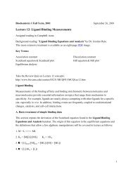
This flow chart summarizes the six approaches:
GraphPad Guide to Comparing Curves. Page 2 of 13

Have you perfromed
the experiment more
than once?
Yes
Can you fit the data
to a model with
linear or nonlinear
regression?
Yes
No
Œ
No, Once
Can you fit the data
to a model with
linear regression,
nonlinear regression,
or neither?
Nonlin
Do you care about a
single best-fit
variable? Or do you
want to compare the
entire curves?
Variable
Curve
Ž
Linear
Neither
‘
Approach 1. Pool several experiments using a best-fit parameter
from nonlinear regression
The first step is to fit each curve using nonlinear regression, and to tabulate the bestfit
values for each experiment. Then compare the best-fit values with a paired t test.
For example, here are results of a binding study to determine receptor number
(Bmax). The experiment was performed three times with control and treated cells
side-by-side. Here are the data:
Experiment Bmax (sites/cell) Control Bmax (sites/cell) Treated
1 1234 987
2 1654 1324
3 1543 1160
Because the control and treated cells were handled side-by-side, analyze the data
using a paired t test. Enter the data into GraphPad InStat, GraphPad Prism (or some
other statistics program) and choose a paired t test. The program reports that the
two-tailed P value is 0.0150, so the effect of the treatment on reducing receptor
number is statistically significant. The 95% confidence interval of the decrease in
receptor number ranges from 149.70 to 490.30 sites/cell.
If you want to do the calculations by hand first compute the difference between
Treated and Control for each experiment. Then calculate the mean and SEM of
those differences. The ratio of the mean difference (320.0) divided by the SEM of
the differences (39.57) equals the t ratio (8.086). There are 2 degrees of freedom
(number of experiments minus 1). You could then use a statistical table to
determine that the P value is less than 0.05.
GraphPad Guide to Comparing Curves. Page 3 of 13

The nonlinear regression program also determined Kd for each curve (a measure of
affinity), along with the Bmax. Repeat the paired t test with the Kd values if you are
also interested in testing for differences in receptor affinity. (Better, compare the
log(Kd) values, as the difference between logs equals the log of the ratio, and it is
the ratio of Kd values you really care about.)
These calculations were based only on the best-fit values from each experiment,
ignoring all the other results calculated by the curve-fitting program. You may be
concerned that you are not making best use of the data, since the number of points
and replicates do not appear to affect the calculations. But they do contribute
indirectly. You’ll get more accurate fits in each experiment if you use more
concentrations of ligand (or more replicates). The best-fit results of the experiments
will be more consistent, which increases your power to detect differences between
control and treated curves. So you do benefit from collecting more data, even
though the number of points in each curve does not directly enter the calculations.
One of the assumptions of a t test is that the uncertainty in the best-fit values follows
a bell-shaped (Gaussian) distribution. The t tests are fairly robust to violations of this
assumption, but if the uncertainty is far from Gaussian, the P value from the test can
be misleading. If you fit your data to a linear equation using linear regression or
polynomial regression, this isn’t a problem. With nonlinear equations, the
uncertainty may not be Gaussian. The only way to know whether the assumption
has been violated is to simulate many data (with random scatter), fit each simulated
data set, and then examine the distribution of best-fit values. With reasonable data
(not too much scatter), a reasonable number of data points, and equations
commonly used by biologists, the distribution of best-fit values is not likely to be far
from Gaussian. If you are worried about this, you could use a nonparametric Mann-
Whitney test instead of a t test.
Approach 2. Pool several experiments without nonlinear regression
With some experiments you may not be able to choose a model, so can’t fit a curve
with nonlinear regression. But even so, you may be able to summarize each
experiment with a single value. For example, you could summarize each curve by
the peak response, the time (or dose) to peak, the minimum response, the difference
between the maximum and minimum responses, the dose or time required to
increase the measurement by a certain amount, or some other value. Pick a value
that matches the biological question you are asking. One particularly useful
summary is the area under the curve, which quantifies cumulative response.
Once you have summarized each curve as a single value, compare treatment
groups with a paired t test. Use the same computations shown in approach 1, but
enter the area under the curve, peak height, or some other value instead of Bmax .
GraphPad Guide to Comparing Curves. Page 4 of 13

Approach 3. Analyze one experiment with nonlinear regression.
Compare best-fit values of one variable.
Even if you have only performed the experiment only once, you can still compare
curves with a t test. A t test compares a difference with the standard error of that
difference. In approaches 2 and 3, the standard error was computed by pooling
several experiments. With approach 3, you use the standard error reported by the
nonlinear regression program. For example, in the first experiment in Approach 1,
Prism reported these results for Bmax:
Best-fit Bmax SE df
Control 1234 98 14
Treated 987 79 14
You can compare these values, obtained from one experiment, with an unpaired t
using InStat or Prism (or any statistical program that can compute t tests from
averaged data). Which values do you enter? Enter the best-fit value of the Bmax as
“mean” and the SE of the best-fit value as “SEM”. Choosing a value to enter for N is
a bit tricky. The t test program really doesn’t need sample size (N). What it needs is
the number of degrees of freedom, which it computes as N-1. Enter “N=15” into
the t test program for each group. The program will calculate DF as N-1, so will
compute the correct P value. The two-tailed P value is 0.0597. Using the
conventional threshold of P=0.05, the difference between Bmax values in this
experiment is not statistically significant.
To calculate the t test by hand, calculate
1234 - 987
t =
= 1.962
2 2
98 + 79
The numerator is the difference between best-fit Bmax values. The denominator is the
standard error of that difference. Since the two experiments were done with the
same number of data points, this equals the square root of the sum of the square of
the two SE values. If the experiments had different numbers of data points, you’d
need to weight the SE values so the SE from the experiment with more data (more
degrees of freedom) gets more weight. You’ll find the equation in reference 1
(applied to exactly this problem) or in almost any statistics book in the chapter on
unpaired t tests.
The nonlinear regression program states the number of degrees of freedom for each
curve. It equals the number of data points minus the number of variables fit by
nonlinear regression. In this example, there were eight concentrations of
radioligand in duplicate, and the program fits two variables (Bmax and Kd). So there
were 8*2 – 2 or 14 degrees of freedom for each curve, so 28 df in all. You can find
the P value from an appropriate table, a program such as StatMate, or by typing this
equation into an empty cell in Excel =TDIST(1.962, 28, 2) . The first parameter is
GraphPad Guide to Comparing Curves. Page 5 of 13

the value of t; the second parameter is the number of df, and the third parameter is
2 because we want a two-tailed P value.
Prism reports the best-fit value for each parameter along with a measure of
uncertainty, which it labels the standard error. Some other programs label this the
SD. When dealing with raw data, the SD and SEM are very different – the SD
quantifies scatter, while the SEM quantifies how close your calculated (sample)
mean is likely to be to the true (population) mean. The SEM is the standard
deviation of the mean, which is different than the standard deviation of the values.
When looking at best-fit values from regression, there is no distinction between SE
and SD. So even if your program labels the uncertainty value “SD”, you don’t need
to do any calculations to convert it to a standard error.
Approach 4. Analyze one experiment with nonlinear regression.
Compare entire curves.
Approach 3 requires that you focus on one variable that you consider most relevant.
If you care about several variables, you can repeat the analysis with each variable fit
by nonlinear regression. An alternative is to compare the entire curves. Follow this
approach.
1. Fit the two data sets separately to an appropriate equation, just like you did in
Approach 3.
2. Total the sum-of-squares and df from the two fits. Add the sum-of-squares from
the control data with the sum-of-squares of the treated data. If your program
reports several sum-of-squares values, sum the residual (sometimes called error)
sum-of-squares. Also add the two df values. Since these values are obtained by
fitting the control and treated data separately, label these values, SSseparate and
DFseparate. For our example, the sums-of-squares equal 1261 and 1496 so SSseparate
equals 2757. Each experiment had 14 degrees of freedom, so DFseparate equals
28.
3. Combine the control and treated data set into one big data set. Simply append
one data set under the other, and analyze the data as if all the values came from
one experiment. Its ok that X values are repeated. For the example, you could
either enter the data as eight concentrations in quadruplicate, or as 16
concentrations in duplicate. You’ll get the same results either way, , provided
that you configure the nonlinear regression program to treat each replicate as a
separate data point.
4. Fit the combined data set to the same equation. Call the residual sum-of-squares
from this fit SScombined and call the number of degrees of freedom from this fit
DFcombmined. For this example, SScombined is 3164 and DFcombmined is 30 (32 data
points minus two variables fit by nonlinear regression).
5. You expect SSseparate to be smaller than SScombined even if the treatment had no
effect simply because the separate curves have more degrees of freedom. If the
two data sets are really different, then the pooled curve will be far from most of
the data and SScombined will be much larger than SSseparate. The question is whether
GraphPad Guide to Comparing Curves. Page 6 of 13

the difference between SS values is greater than you’d expect to see by chance.
To find out, compute the F ratio using the equation below, and then determine
the corresponding P value (there are DFcombined-DFseparate degrees of freedom in the
numerator and DFseparate degrees of freedom in the denominator.
( SScombined
− SSseparate
) ( DFcombined
− DFseparate
)
F =
SSseparate
DF
For the example, F=2.067 with 2 df in the numerator and 28 in the denominator.
To find the P value, use a program like GraphPad StatMate, find a table in a
statistics book, or type this formula into an empty cell in Excel =FDIST(2.067,2,28)
. The P value is 0.1463.
The P value tests the null hypothesis that there is no difference between the control
and treated curves overall, and any difference you observed is due to chance. If the
P value were small, you would conclude that the two curves are different – that the
experimental treatment altered the curve. Since this method compares the entire
curve, it doesn’t help you focus on which parameter(s) differ between control and
treated (unless, of course, you only fit one variable). It just tells you that the curves
differ overall. If you want to focus on a certain variable, such as the EC50 or
maximum response, then you should use a method that compares those variables.
Approach 4 compares entire curves, so the results can be hard to interpret.
In this example, the P value was fairly large, so we conclude that the treatment did
not affect the curves in a statistically significant manner.
separate
Approach 5. Compare linear regression lines
If your data form straight lines, you can fit your data using linear regression, rather
than nonlinear regression. JH Zar discusses how to compare linear regression lines
in reference 2. Here is a summary of his approach:
First compare the slopes of the two linear regression lines using a method similar to
approach 3 above. Pick a threshold P value (usually 0.05) and decide if the
difference in slopes is statistically significant.
• If the difference between slopes is statistically significant, then conclude that the
two lines are distinct. If relevant, you may wish to calculate the point where the
two lines intersect.
• If the difference between slopes is not significant then fit new regression lines
but with the constraint that both must share the same slope. Now ask whether
the difference between the elevation of these two parallel lines is statistically
significant. If so, conclude that the two lines are distinct, but parallel. Otherwise
conclude that the two lines are statistically indistinguishable.
GraphPad Guide to Comparing Curves. Page 7 of 13

The details are tedious, so aren’t repeated here. Refer to the references, or use
GraphPad Prism, which compares linear regression lines automatically.
An alternative approach to compare two linear regression lines is to use multiple
regression, using a dummy variable to denote treatment group. This approach is
explained in reference 3, which also describes, in detail, how to compare slopes
and intercepts without multiple regression.
Approach 6. Comparing curves with ANOVA
If you don’t have enough data points to allow curve fitting, or if you don’t want to
choose a model (equation), you can analyze the data using two-way analysis of
variance (ANOVA) followed by posttests. This method is also called two-factor
ANOVA (one factor is dose or time; the other factor is experimental treatment).
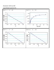
Here is an example, along with the two-way ANOVA results from Prism.
Dose
0.0
1.0
2.0
Control
Y1 Y2 Y3
23.0
34.0
43.0
25.0
41.0
47.0
29.0
37.0
54.0
Treated
Y1 Y2 Y3
28.0
47.0
65.0
31.0
54.0
60.0
26.0
56.0
75
Response
50
25
0
Control
Treated
0 1 2
Dose
Source of Variation
Interaction
Treatment
Dose
P value
0.0384
0.0002
P

Two-way ANOVA computes three P values.
• The P value for interaction tests the null hypothesis that the effect of treatment is
the same at all doses (or, equivalently, that the effect of dose is the same for
both treatments). This P value is below the usual threshold of 0.05, so you can
conclude that the null hypothesis is unlikely to be true. Instead, the effect of
treatment varies significantly with dose. The dose-response curves are not
parallel.
• The P value for treatment tests the null hypothesis that the treatments have no
effect on the response. This P value is very low, so you conclude that treatment
did affect response on average. The dose-response curves are not identical.
When the interaction P value is low, it is hard to interpret the P value for
treatment.
• The P value for dose tests the null hypothesis that dose had no effect on the
response. It is very low, so you conclude that response varied with dose. The
dose-response curves are not horizontal. When the interaction P value is low, it
is hard to interpret the P value for dose.
Since the treatment had a significant effect, and had a different effect at different
doses, you may now wish to perform posttests to determine at which doses the
effect of treatment is statistically significant. The current version (2.0) of GraphPad
Prism does not perform any posttests following two-way ANOVA, but the next
version (3.0) will. Other ANOVA programs perform posttests, but often not the
posttests you need to compare dose-response curves. Instead, most programs pool
the control and treated values to determine the mean response at each dose, and
then perform posttests to compare the average response at one dose with the
average response at another dose. This approach is useful in many contexts, but not
when comparing dose-response or kinetic curves. Fortunately, it is fairly
straightforward to perform the posttest calculations by hand.
Your first temptation may be to perform a separate t test at each dose, but this
approach is not appropriate. Instead, compute posttests as explained in reference 4.
At each dose (or time point), compute:
t =
mean − mean
MS
1
residual
⎛ 1
⎜
⎝ N
1
2
1
+
N
2
⎞
⎟
⎠
The numerator is the mean response in one group minus the mean response at the
other group, at a particular dose (or time point). The mean is computed from
replicate values at one dose (or time) from one treatment group. The denominator
combines the number of replicates in the control and treated samples at that dose
with the mean square of the residuals (sometimes called the mean square of the
GraphPad Guide to Comparing Curves. Page 9 of 13

error), which is a pooled measure of variability at all doses. One of the assumptions
of two-way ANOVA is that the variability (experimental error) is the same for each
dose for each treatment. If this is not a reasonable assumption, you may be able to
transform the values – perhaps as logarithms – so it is. If you assume that the
variability is the same for all doses and all treatments, then it makes sense to pool
all the variability into one number, the MSresidual. Some programs call this value
MSerror.
In the example, MSresidual equals 15.92, a value you can read off the ANOVA table.
Here are the results at each of the three doses. The means and sample sizes are
computed directly from the data table shown above, and the t ratio is then
computed for each dose.
Dose Mean 1 Mean 2 N 1 N 2 t
0 25.7 28.3 3 3 0.8185
1 37.3 52.3 3 3 4.6048
2 48.0 62.5 3 2 3.9809
Which of these differences are statistically significant? To find out, we need to know
the value of t that corresponds to P=0.05, correcting for the fact that we are making
three comparisons. You can get this critical t value from Excel by typing this
formula into a blank cell: =TINV(0.05/3, 11) . The first parameter is the
probability. We entered 0.05/3, because we wanted to set α to its conventional
value of 0.05, but adjusted to account for three simultaneous comparisons (there
were three doses in this example). You could enter a different value than 0.05 or a
different number of doses (or time points). The second parameter is the degrees of
freedom, which you can see on the ANOVA table (df for residuals). The critical t
value is 2.8200.
The t ratio at time 0 is less than 2.82, so that difference is not statistically significant.
The t ratio at the other two times are greater than 2.82, so are significant at the 0.05
level, correcting for multiple comparisons. The threshold t ratio for significance at
the 0.01 level is computed as TINV(0.01/3,11) which equals 3.728. The differences
at doses 1 and 2 are significant at the 0.01 level. The t ratio for significance at the
0.001 level is 5.120, so none of the differences are significant at the 0.001 level.
The value 5% refers to the entire family of comparisons, not to each individual
comparison. If the treatment had no effect, there is a 5% chance that random
variability in your data would result in a statistically significant difference at any one
or more doses, and thus a 95% chance that the treatment would have a
nonsignificant effect at all doses. This correction for multiple comparisons uses the
method of Bonferroni (divide 0.05 by the number of comparisons).
GraphPad Guide to Comparing Curves. Page 10 of 13

You can also calculate a confidence interval for the difference between control and
treated values at each dose using this equation:
*
⎛ 1 1 ⎞
*
⎛ 1 1 ⎞
(mean − ⋅
⎜ +
⎟
− + ⋅
⎜ +
⎟
2
mean1)
- t MSresidual
to (mean
2
mean1)
t MSresidual
⎝ N1
N
2 ⎠
⎝ N1
N
2 ⎠
The critical value of t is abbreviated t* in that equation (not a standard
abbreviation). Its value was determined above as 2.8200. The value depends only
on the number of degrees of freedom and the degree of confidence you want.
You’d get a different value for t* if you have a different number of degrees of
freedom. Since that value of t* was determined for a P value of 0.05, it generates
95% confidence intervals (100%-5%). If you picked t* for P=0.01, that value could
be used for 99% confidence intervals.
The value of MSresidual is found on the ANOVA table; it equals 15.92. Now you can
calculate the lower and upper confidence limits at each dose:
Dose mean 1 Mean 2 N 1 N 2 Lower CL Upper CL
0 25.7 28.3 3 3 -6.59 11.79
1 37.3 52.3 3 3 5.81 24.19
2 48.0 62.5 3 2 4.23 24.77
Because the value of t* used the Bonferroni correction, these are simultaneous 95%
confidence intervals. You can be 95% sure that all three of those intervals contain
the true effect of treatment at that dose. So you can be 95% sure that all three of
these statements are true: The effect of dose 0 is somewhere between a decrease of
6.59 and an increase of 11.79; dose 1 increases response between 5.81 and 24.19;
and dose 2 increases response between 4.23 and 24.77.
Note that this method assumes that the Y1, Y2 and Y3 values entered into the data
table represent triplicate measurements, and that there is no matching. In other
words, it assumes that the Y1 measurement for the first time point is not matched to
the Y1 measurement for the second time point. If all the Y1 measurements are from
matched experiments, or from one individual repeatedly measured, then you’ll
need an ANOVA program that can handle repeated measures. You’ll get a different
value for the residual sum-of-squares and degrees of freedom, but can perform the
posttest in the same way.
Using two-way ANOVA to compare dose-response curves presents two problems.
One problem is that ANOVA treats different doses (or time points) exactly as it
treats different species or different drugs. ANOVA ignores the fact that doses or time
points come in order. If you jumbled the order of the doses, you’d get exactly the
same ANOVA results. You did the experiment to observe a trend, so you should be
cautious about interpreting results from an analysis method that doesn’t recognize
trends.
GraphPad Guide to Comparing Curves. Page 11 of 13

Another problem with the ANOVA approach is that it is hard to interpret the results.
Knowing at which doses or time points the treatment had a statistically significant
effect doesn’t always help you understand the biology of the system, and rarely
helps you design new experiments. Some scientists like to ask which is the lowest
dose (or time) at which the effect of the treatment is statistically significant. The
posttests give you the answer, but the answer depends on sample size. Run more
subjects, or more doses or time points for each curve, and the answer will change.
This ANOVA method is most useful when you have collected data at only a few
doses or time points. For experiments where you collect data at many doses or time
points, consider one of the other approaches.
Comparing more than two curves
This article focussed on comparing two curves. If you have several treatment
groups, approaches 1-3 can easily be extended to handle three or more groups.
Simple use one-way ANOVA, rather than a t test. Extending approaches 4-6 to
handle three or more groups is more difficult, beyond the scope of this article.
Summary
How do you test whether an experimental manipulation changed the dose-response
(or some other) curve? This is a common question, but one that requires a long
answer. The best approach is to summarize each curve with a single value, and
then compare treatment groups with a t test. If you’ve only performed the
experiment once, you’ll need to use another approach and this article lists several.
But you’ll probably want to repeat the experiment before reaching a strong
conclusion.
GraphPad Software
The author of this article is the president of GraphPad Software, creators of
GraphPad Prism and GraphPad InStat.
GraphPad Prism is a scientific graphics program that is particularly well suited for
nonlinear regression:
• Prism provides a menu of commonly used equations (including equations used
for analysis of radioligand binding experiments). To fit a curve, all you have to
do is pick the right equation. Prism does all the rest automatically, from picking
initial values to graphing the curve.
• Prism can automatically compare two models with the F test.
• When analyzing competitive radioligand binding curves, Prism automatically
calculates Ki from IC50.
• You can use the best-fit curve as a standard curve. Enter Y values and Prism will
determine X; enter X and Prism will determine Y.
GraphPad Guide to Comparing Curves. Page 12 of 13

• Prism can automatically graph a residual plot and perform the runs test.
• Prism’s manual and help screens explain the principles of curve fitting with
nonlinear regression and help you interpret the results. You don’t have to be a
statistics expert to use Prism.
GraphPad InStat is a low-end statistics program. It is so easy to use that anyone can
master it in about two minutes – really. InStat helps you choose an appropriate
statistical test and helps you interpret the results. It even shows you an analysis
checklist to be sure that you’ve picked an appropriate test.
Please visit GraphPad’s web site at http://www.graphpad.com. You can read about
Prism and InStat and download free demos. The demos are not slide shows – they
are functional versions of Prism and InStat with no limitations in data analysis. Try
them with your own data, and see for yourself why Prism is the best solution for
analyzing and graphing scientific data and why InStat is the world’s simplest
statistics program.
While at the web site, browse the GraphPad Data Analysis Resource Center. You’ll
find the GraphPad Guide to Nonlinear Regression and the GraphPad Guide to
Analyzing Radioligand Binding Data, along with shorter articles. You’ll also find a
radioactivity calculator and links to recommended web sites and books.
References
1. SA Glantz, BK Slinker, Primer of Applied Regression and Analysis of Variance,
McGraw-Hill, 1990. Page 504 explains approach 3, and gives the equation to
use when the two treatments were analyzed with different numbers of data
points.
2. J Zar, Biostatistical Analysis, 2nd edition, Prentice-Hall, 1984. Chapter 18
explains approach 5.
3. DG Kleinbaum and LL Kupper, Applied Regression Analysis and Other
Mutivariable Methods, Duxbury Press , 1997. Gives the details of approach 5,
and also how to compare linear regression lines using multiple regression.
4. J Neter, W Wasserman, MH Kutner, Applied Linear Statistical Models. 3 rd
edition, Irwin, 1990. Pages and 741-744 and 771 explain approach 6.
GraphPad Guide to Comparing Curves. Page 13 of 13