Advances in perturbative thermal field theory - Ultra-relativistic ...

410 U Kraemmer and A Rebhan
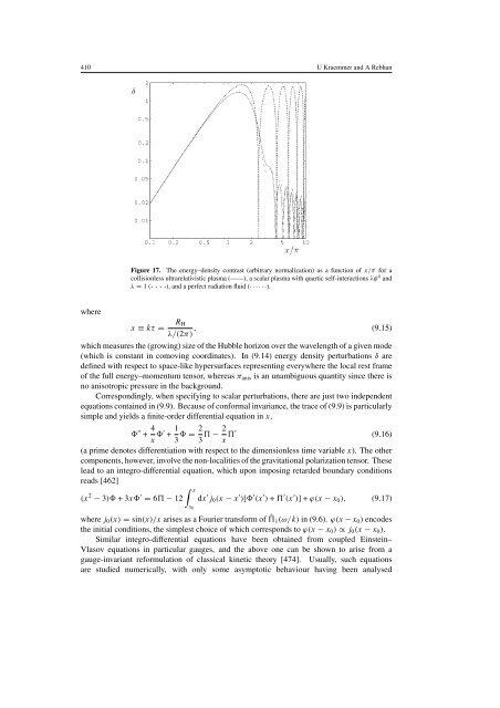
Figure 17. The energy–density contrast (arbitrary normalization) as a function of x/π for a
collisionless ultrarelativistic plasma (——), a scalar plasma with quartic self-interactions λφ 4 and
λ = 1 (- - - -), and a perfect radiation fluid (······).
where
x ≡ kτ =
R H
λ/(2π) , (9.15)
which measures the (growing) size of the Hubble horizon over the wavelength of a given mode
(which is constant in comoving coordinates). In (9.14) energy density perturbations δ are
defined with respect to space-like hypersurfaces representing everywhere the local rest frame
of the full energy–momentum tensor, whereas π anis is an unambiguous quantity since there is
no anisotropic pressure in the background.
Correspondingly, when specifying to scalar perturbations, there are just two independent
equations contained in (9.9). Because of conformal invariance, the trace of (9.9) is particularly
simple and yields a finite-order differential equation in x,
′′ + 4 x ′ + 1 3 = 2 3 − 2 x ′ (9.16)
(a prime denotes differentiation with respect to the dimensionless time variable x). The other
components, however, involve the non-localities of the gravitational polarization tensor. These
lead to an integro-differential equation, which upon imposing retarded boundary conditions
reads [462]
∫ x
(x 2 − 3) +3x ′ = 6 − 12 dx ′ j 0 (x − x ′ )[ ′ (x ′ ) + ′ (x ′ )]+ϕ(x − x 0 ), (9.17)
x 0
where j 0 (x) = sin(x)/x arises as a Fourier transform of ˆ 1 (ω/k) in (9.6). ϕ(x − x 0 ) encodes
the initial conditions, the simplest choice of which corresponds to ϕ(x − x 0 ) ∝ j 0 (x − x 0 ).
Similar integro-differential equations have been obtained from coupled Einstein–
Vlasov equations in particular gauges, and the above one can be shown to arise from a
gauge-invariant reformulation of classical kinetic theory [474]. Usually, such equations
are studied numerically, with only some asymptotic behaviour having been analysed