The Physical Basis of The Direction of Time (The Frontiers ...

2.1 Retarded and Advanced Form of the Boundary Value Problem 21
t 2
t
P
t 1
x
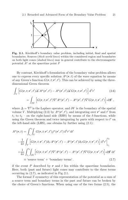
Fig. 2.1. Kirchhoff’s boundary value problem, including initial, final and spatial
boundaries. Sources (thick world lines) within the considered region and boundaries
on both light cones (dashed lines) may in general contribute to the electromagnetic
potential A µ at the spacetime point P
By contrast, Kirchhoff’s formulation of the boundary value problem allows
one to express every specific solution A µ (r,t) of the wave equation by means
of any Green’s function G(r,t; r ′ ,t ′ ). This can be achieved by using the threedimensional
Green theorem
∫ [
]
G(r,t; r ′ ,t ′ )∆ ′ A µ (r ′ ,t ′ ) − A µ (r ′ ,t ′ )∆ ′ G(r,t; r ′ ,t ′ ) d 3 r ′ (2.6)
V
∫
=
∂V
[
]
G(r,t; r ′ ,t ′ )∇ ′ A µ (r ′ ,t ′ ) − A µ (r ′ ,t ′ )∇ ′ G(r,t; r ′ ,t ′ ) ·dS ′ ,
where ∆ = ∇ 2 is the Laplace operator, and ∂V is the boundary of the spatial
volume V . Multiplying (2.3) by A µ (r ′ ,t ′ ), and integrating over r ′ and t ′ from
t 1 to t 2 – on the right-hand side (RHS) by means of the δ-functions, while
using the Green theorem and twice integrating by parts with respect to t ′ on
the left-hand side (LHS), one obtains by further using (2.1):
A µ (r,t)=
− 1 ∫
4π V
+ 1
4π
∫ t2
∫ t2
t 1
∫V
G(r,t; r ′ ,t ′ )j µ (r ′ ,t ′ )d 3 r ′ dt ′
[
G(r,t; r ′ ,t ′ )∂ t ′A µ (r ′ ,t ′ ) − A µ (r ′ ,t ′ )∂ t ′G(r,t; r ′ ,t ′ )
t 1
∫∂V
]
d 3 r ′ ∣ ∣∣∣
t 2
[
]
G(r,t; r ′ ,t ′ )∇ ′ A µ (r ′ ,t ′ ) − A µ (r ′ ,t ′ )∇ ′ G(r,t; r ′ ,t ′ ) ·dS ′ dt ′
≡ ‘source term’ + ‘boundary terms’ . (2.7)
if the event P described by r and t lies within the spacetime boundaries.
Here, both (past and future) light cones may contribute to the three terms
occurring in (2.7), as indicated in Fig. 2.1.
The formal T -symmetry of this representation of the potential as a sum of
a source term and boundary terms in the past and future can be broken by
the choice of Green’s functions. When using one of the two forms (2.5), the
t 1