Linear Differential Game With Two Pursuers and One Evader

Linear Differential Game With Two Pursuers and One Evader
Stéphane Le Ménec
stephane.le-menec@mbda-systems.com
EADS / MBDA France
Abstract
We study the situation involving two pursuers and one evader in the framework of DGL/1 (Linear
Differential Game with bounded controls and first order dynamics for both players). A new optimal
evasion strategy is then derived to compromise the terminal miss distance respect to each pursuer. This
trade off strategy and the resulting 2x1 No Escape Zone have been computed when the pursuers have
same time-to-go as well as with different time-to-go.
1. Introduction
We consider head on scenarios with two pursuers (P1 and P2) and one evader (E). The purpose of this
paper is to compute two on one differential game No Escape Zones (NEZ) [8]. The main objective
(over the scope of this paper) consists in designing suboptimal strategies in many on many
engagements. 1x1 NEZ and 2x1 NEZ are components involved in suboptimal approaches we are
interested in (i.e. “Moving Horizon Hierarchical Decomposition Algorithm” [6]). Several specific two
pursuers one evader differential games have been already studied ([1], [4], [7]). Nevertheless, we
propose to compute 2x1 NEZ from 1x1 DGL/1 NEZ because DGL models are games with well
defined analytical solutions [12].
2. One on one DGL/1 game
For reminder, we briefly summarize some results about one on one pursuit evasion game using DGL/1
models. DGL/1 differential games are co planar interceptions with constant velocities, bounded
controls assuming small motion variations around the collision course triangle. Under this assumption
the kinematics is linear. Each player is represented as a first order system (time lag constant). The
criterion is the terminal miss distance (terminal cost only, absolute value of the terminal miss
perpendicular to the initial Line Of Sight, LOS). DGL/1 are fixed time duration differential games,
with final time defined by the closing velocity (assumed constant) and the pursuer evader range. The
terminal projection procedure [3] allows to reduce the initial four dimension state vector representation
to a scalar representation and to represent the optimal trajectories in the ZEM (Zero Effort Miss), Tgo
(Time to Go) coordinate frame. According to notations and normalizations defined in [12] the DGL/1
kinematics is as follow:
d z
⎛θ
⎞
= μ h( θ ) u − ε h⎜
⎟ v
d θ
⎝ ε ⎠
( ) = − α
h α e + α −1
aP
max
τ
E
μ = , ε =
a τ
In this framework,
a
a
Pc
u = and
P max
a
a
E max
E max
P
Ec
v = are respectively the pursuer and evader controls
( u ≤ 1, v ≤ 1). aP
max
and aE
max
are the maximum accelerations. a Pc
and a Ec
are the lateral
accelerations demands. τ P
and τ E
are the pursuer and evader time lag constants. The independent
variable is the normalized time to go:
τ
θ = , τ = t f
− t
τ
P
Where t
f
is the final time. The non-dimensional state variable is the normalized Zero Effort Miss :
- 1 -

ZEM
z ( θ ) =
2
τ
P
a E max
The Zero Effort Miss distance is given below for DGL/1:
2
2 ⎛θ
⎞
ZEM ( t)
= y + y&
t − && y τ h( θ ) + & y
go P P
E
τ
E
h⎜
⎟
⎝ ε ⎠
Where y is the relative perpendicular miss, y& the relative perpendicular velocity, & y& P
the
(instantaneous) perpendicular pursuer acceleration and & y&
E
the perpendicular evader acceleration. The
non-dimensional cost function is the normalized terminal miss distance subject to minimization by the
pursuer and maximization by the evader.
= z = z θ = 0
J
f
( t)
( )
The (ZEM, Tgo) frame is divided into two regions, the regular area and the singular one. For some
appropriated differential game parameters (pursuer to evader maximum acceleration ratio μ and evader
to pursuer time lag ratio ε), the singular area plays the role of capture zone so called also NEZ (leading
to zero terminal miss), whilst the regular area corresponds to the non capture zone. The NEZ can be
bounded (closed) or unbounded (open). The natural optimal strategies are bang-bang controls
corresponding to the sign of ZEM (some refinements exist when defining optimal controls inside the
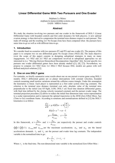
NEZ). We start the 2x1 DGL/1 analysis with unbounded 1x1 NEZ as pictured in Figure 1 (NEZ
delimited by the two plain red lines, non capture zone corresponding to the state space filled with
optimal trajectories in dot blue lines). Moreover, we first assume same Tgo in each DGL/1 game
(same initial range, same velocity for each pursuer).
300
DGL/1, μ = 3.6, ε = 0.8, με = 2.88
200
100
z * + (τ)
normalized z
0
-100
z * - (τ)
-200
-300
0 5 10 15
normalized tgo
Figure 1 : Unbounded NEZ (ZEM, Tgo frame)
3. Two pursuers one evader DGL/1 game
3.1. Criterion
The outcome we consider in the 2x1 game is the minimum of the two terminal miss distances.
With J the terminal miss,
i
( u u , v) min { J ( u , v) , J ( u v)
}
J x
,
2 1 1, 2
=
1
2
u the control of Pi , = { 1, 2}
( u v)
( u v)
( u u v)
i and v the evader control.
J
1
, : P1 E DGL/1 terminal miss
J
2
, : P2 E DGL/1 terminal miss
J
2 x 1 1,
2,
: 2x1 DGL/1 outcome
- 2 -

The 2x1 game only makes a change in the evader optimal command. The presence of a second pursuer
doesn’t change the pursuers behaviour. Indeed, the optimal controls for each pursuer in the 2x1 game
are the same as the ones in their respective 1x1 game.
When considering two pursuers and one evader (in the framework of DGL representations), some
cases are easy to solve. If E is “above” (or symmetrically “below”) the two pursuers (in ZEM, Tgo
frame), the optimal evasion respect to each pursuer (considered alone) and according to both pursuers
together is to turn right (to turn left when below) with maximum acceleration. In these cases (E
“above” or “below”), there are no changes in evasion trajectory (optimal strategies) by adding a
pursuer.
ZEM
P1
E
P1E Reference
P2
P2E Reference
Figure 2 : 2x1 game with Evader between the two Pursuers (ZEM, Tgo frame)
For the other initial conditions (see Figure 2) we have to refine the optimal evasion behaviour. If E is
between P1 and P2 (as described in Figure 2) then the optimal 2x1 evasion is a trade off between the
incompatible P1 E and P2 E optimal escapes. Notice that in Figure 2 the initial LOS (in each DGL/1
game) have been chosen parallel.
3.2. Trade off evader control
* * *
We compute the 2x1 DGL/1 game solution ( ( u u v
)
J
2 x1
1
,
2
,
2x1
considering that the optimal evasion
control is a constant value during the entire game and considering that the terminal miss distances
respect to P1 and P2 have to be the same (for initial conditions outside the NEZ and when no control
*
*
*
saturation occurs). In the case of Figure 2, v = 1 (left turn), v 1 (right turn) and −1
≤ v 1.
J
J
J
2x1
* *
( u1
, v2
)
* *
( u2
, v1
)
* *
( u , u , v)
1
2
≤ J
2x1
1
−
2
=
* * *
* *
* *
( u , u , v ) = J ( u , v ) = J ( u , v )
1
2
2x1
1
2x1
2
2x1
J
≤
J
* *
( u1
, v1
)
* *
( u , v )
2
2
2x1
≤
According to notations and normalizations detailed in the previous section, we write the final distances
equality condition in the following manner (where Z are the ZEM in each PE game) :
( t ) = Z ( t )
Z1 f
−
2
Note that the minus sign is due to the y-axes orientation like in Figure 2. In normalized variable, we
get (with τ
Pi
the Pursuer time lag constants) :
2
2
z τ = −z
τ , z = z τ 0
i
f
( ( ))
1 f P1
2 f P2
if i
=
Looking at Figure 3, the normalized zero-effort-miss at final time can be written (where
distance diminutions due to application of sub optimal evader controls):
Δz
are miss
- 3 -

( τ ) + z1max
( τ ) + Δz1( 0)
( τ ) − z ( τ ) + Δz
( 0)
z1 f
= z1
τ =
z2 f
= z2
2 max
2
τ =
In Figure 3, for simplicity reasons we plot the 2x1 game in the ZEM Tgo frame on one unique figure.
It is done by superimposition of the two plots of each couple pursuer-evader with the game initial
condition as point of coincidence (P2 located at origin and P1 located at x = 0 and y = 11000 ), even
if during the game, the Δ P1 P2 range decreases.
12000
10000
-z 1max
8000
Δ z
v* 2x1
Distance (m)
6000
4000
v* 1x1
= -1
2000
0
0 1 2 3 4 5 6 7 8 9 10
τ go
(s)
Figure 3 : Calculation of
*
v
2x1
The 1x1 DGL/1 no-escape-zone expressions are well known [12] :
Where:
and
H
2
H
z
H
1
z
= μ
− ε
1max
1H11
1H
21
2 max
= μ
2
H12
− ε
2H
22
( θ , ε ),
1, 2
1 , i
= H1
i
i =
θ
2
θ
= ∫
2
( θ ) h( ξ ) dξ
= − h( θ )
H
0
( θ , ε ),
1, 2
2 , i
= H
2 i
i =
θ
2
ξ θ θ
= ∫ ⎜ ⎟
⎜
⎝ ε ⎠ 2 ε ⎝ ε
⎛ ⎞
⎛ ⎞
( θ ) h dξ
= − ε h ⎟
⎠
0
The third terms
Δ zi
that corresponds to the changes in z
if
due to
Δ
Δz
Substituting these expressions lead to:
ε
*
v
2x1
are:
* *
*
( v2x
1
− v1x
1
) = ε1H
21( v2x
1
1)
* *
*
( v − v ) = ε H ( v 1)
z1 =
1H
21
+
2
= ε
2H
22 2x1
1x1
2 22 2x1
−
- 4 -

*
( μ
1H
11
− ε
1H
21
) + ε
1H
21( v2
1
1)
*
( μ H − ε H ) + ε H ( v 1)
z1 f
= z1
+
x
+
2 f
= z
2
−
2 12 2 22 2 22 2x1
−
z
From which, using the initial equality, we can isolated
the evader bounds) :
v
*
2×
1
( z)
=
*
v
2x1
(subject to saturation if
2
( − μ H − z ) τ + ( μ H − z )
1
ε
11
2
H
1
22
τ
P1
2
P2
+ ε
2 12 2
2
1
H
21
τ
P1
τ
2
P2
*
v
2x1
is higher than
*
v
2x1
is relevant outside the 2x1 NEZ and is a “reasonable” solution inside the capture zone too. Figure
4 illustrates the optimal trajectories we obtain when the time to go are the same for each pursuer
( μ1
= 2, ε1
= 2, μ2
= 3, ε
2
= 0.85714).
4000
2000
P1
P2
E
0
Distance Y [m]
-2000
-4000
-6000
-8000
0 0.5 1 1.5 2 2.5 3 3.5
Distance X [m]
x 10 4
Figure 4 : Example with evader playing
*
v
2x1
3.3. Two on One No Escape Zone
The overall 2x1 NEZ is the collection of P1 E NEZ plus P2 E NEZ plus an extra state space area. If
the evader plays in the worst way (from the evader point of view) vi = -sign( z
i
) then a new limit is
under consideration. In addition to z
i max
we define z
i min
:
z1min
= μ
1H11
+ ε
1H
21
z = μ H + ε
2 min 2 12 2H
22
The new 2x1 frontier is then the line between the two intersections that are solution of the equations:
z θ = −z
θ + ΔP
z
( )
1min
( )
1 2
( θ ) = −z1max
( θ ) + ΔP1
2
2 max
P
2 min
P
These two equations give an unique solution τ
2x1
which characterizes the new barrier in the 2x1 game.
Figure 5 shows the boundary of the 2x1 game ( τ
2x1
≈ 7.2 sec. ) with same parameters as in previous
section. The state space area outside the two 1x1 NEZ (blue plain lines) but with τ ≥ τ 2x 1
(vertical red
line) is also now belonging to the 2x1 NEZ.
- 5 -

11000
10000
9000
8000
7000
Distance [m]
6000
5000
4000
3000
2000
1000
0
0 2 4 6 8 10 12
τ go
[s]
Figure 5 : NEZ extension in 2x1 game
Figure 6 characterizes the saturations that apply in the evader optimal controls. Outside the 2x1
capture zone (always still considering E between the two pursuers) three different end games can
happen:
If z
1 f
= 0 and z
2 f
= 0 then the initial conditions belong to the 2x1 no-escape-zone.
If z
if
≠ 0 and z1 f
= z2
f
then the initial conditions belong to the 2x1 non-saturate zone (area in red in
Figure 6).
If z
if
≠ 0 and z1 f
≠ z2
f
then the initial conditions belong to the 2x1 saturate zone (case
corresponding to the “trade off” evader controls overcoming the control bounds).
12000
10000
8000
ZEM [m]
6000
4000
2000
0
0 1 2 3 4 5 6 7 8 9 10
τ go
[s]
Figure 6 : Evader control saturation
*
This new limit, as well as the zone of v
2x1
saturation, have been investigated in linear and non-linear
simulations in order to confirm the computation of τ
2x1. Up to now, the 2x1 game trajectories (Figure
3, Figure 5, Figure 6) have been plotted on a single ( ZEM , τ
go
) representation. Figure 7 represents
ZEM , τ go
, ΔP1P2
. On the left side delimited by the
the barrier of the 2x1 game in the state space ( )
red surface P2 intercepts E. On the right part (delimited by the blue surface) E is captured by P1. The
capture zone extension due to the presence of two pursuers is depicted by green and purple lines.
- 6 -

Moreover, in Figure 7 we draw an optimal trajectory (black line) starting (and remaining) on the new
2x1 boundary.
2x1 DGL/1 NEZ + optimal trajectory on the barrier
12000
10000
delta P1P2 [m]
8000
6000
4000
10
2000
0
-2000 0
2000 4000
6000 8000 10000 0
ZEM [m]
12000
5
Time to Go [sec]
Figure 7 : 2x1 NEZ
3.4. Case of different time to go
In this configuration, the two pursuers are launched at different times and so different time-to-go. The
*
previous expression of v
2x1
is no longer available and thus need to be generalized to take into account
the difference in time-to-go. Note that in this new case, the evader is assumed to switch its command
*
to v
1x1
(and faces only one pursuer like in a 1x1 game) when it goes beyond the first opponent. The
*
optimal evader control, always called v
2x1
, should still lead to the equality of the final distances (in
absence of evader control saturations):
Z τ = = −Z
τ 0
12000
(
1
0) 2( 2
)
2
2
( ) τ = −z
( ) τ
1
=
z1 0
P1
2
0
P2
10000
-z 1max
z 2max
8000
Δ z 1
v* 2x1
6000
4000
2000
Δτ
Δ z 2
v* 1x1
= -1
0
0 1 2 3 4 5 6 7 8 9 10
Figure 8 : Calculation of
v with different time-to-go (
2
τ
1
*
2x1
- 7 -
τ < )

Looking at Figure 8, case where τ
2
< τ
1
, the normalized zero-effort-miss at final time can be now
written:
z
1( 0) = z1( τ
1
) + z1max
( τ
1
) + Δz1( Δτ
)
z = z τ − z τ + Δ 0
Since ( ) = Δ ( Δτ )
( ) ( ) ( ) ( )
2
0
2 2 2 max 2
z
2
Δ 0 z
*
z
1 1
because evader plays only against P1 ( v
1x1
= −1) during Δ τ (see Figure 8).
Notice that in Figure 8 the x axis corresponds to τ 1
values ( τ
2
+ Δτ ) . The third terms that
*
corresponds to the new change in due to v
2x1
is:
Δz
z 1 f
And, thanks to the properties of integrals,
H
21
* *
( Δτ
) = ε H ( Δτ
→ τ ) ( v − v )
1 1 21
1 2x1
1x1
θ
⎛ ξ ⎞
⎜ ⎟
⎝ ε ⎠
1
( Δτ
→ τ ) = h dξ
= H ( τ ) − H ( Δτ
)
1
∫
Δτ
21
1
21
Expression becomes:
Δz
*
[ ]( v 1)
( Δτ
) = ε H ( τ ) − ε H ( Δτ
)
1 1 21 1 1 21
2x1
+
Substituting these expressions leads to:
z
*
( ) = z ( τ ) + μ H ( τ ) − ε H ( Δτ
) + [ ε H ( τ ) − ε H ( Δτ
)] v
1
0
1 1 1 11 1 1 21
1 21 1 1 21
2x1
Moreover, the expression of
z
z 2 f
remain the same as before when time to go coincided:
*
[ ] + ε H ( τ ) ( v 1)
( 0) z ( τ ) − μ H ( τ ) − ε H ( τ )
2
=
2 2 2 12 2 2 22 2 2 22 2 2x1
−
From which, using the initial equality, we can isolated
v , in the case where τ
2
< τ
1
:
*
2x1
v
*
2×
1
( z)
=
2
[ − μ1
H
11( τ
1
) − z1( τ
1
) + ε
1H
21( Δτ
)] τ
P1
+ [ μ
2
H
12
( τ
2
) − z
2
( τ
2
)]
2
2
ε H ( τ ) τ + [ ε H ( τ ) − ε H ( Δτ
)] τ
2
22
2
P2
1
21
1
1
21
P1
τ
2
P2
Due to the problem symmetry, the same calculus can be done switching the role of pursuers 1 and 2.
Expression of v in case where τ
2
> τ
1
is then as follow:
v
*
2×
1
( z)
*
2x1
=
2
[ − μ1
H
11( τ
1
) − z1( τ
1
)] τ
P1
+ [ μ
2
H
12
( τ
2
) − ε
2
H
22
( Δτ
) − z
2
( τ
2
)]
2
2
[ ε H ( τ ) − ε H ( Δτ
)] τ + ε H ( τ ) τ
2
22
2
2
22
*
Note that the particular case where Δτ = 0 leads to the expression of v
2x1
found in section 3.2 (same
time to go). By the way, we compute the 2x1 NEZ extension when time to go differs. Figure 9 and
Figure 10 show τ
2x1
limit remaining as a straight line (dash red line in Figure 9). The green crosses in
Figure 10 represent an optimal trajectory on the 2x1 NEZ boundary at different time instants.
P2
1
21
1
P1
τ
2
P2
- 8 -

12000
10000
8000
ZEM [m]
6000
4000
2000
0
0 2 4 6 8 10 12
τ go
[s]
−τ
Figure 9 : 2x1 NEZ for 1 sec.
τ
1 2
=
10000
10000
ZEM [m]
5000
5000
4000
0
0 5 10
4000
0
0 5 10
ZEM [m]
3000
2000
1000
1000
0
0 2 4 6
3000
2000
1000
1000
0
0 2 4 6
ZEM [m]
500
500
0
0 1 2 3 4 5
τ go
[s]
0
0 1 2 3 4 5
τ go
[s]
Figure 10 : 2x1 NEZ sections at different time instants.
4. Conclusion
We extend DGL/1 to the three players game involving two pursuers and one evader. We solve the
game showing that for some initial conditions located between the pursuers the optimal evasion
strategy is no more a maximum turn control. The optimal evasion consists then in a “trade off”
strategy to drive the evader between the two pursuers. Considering 2x1 games we enlarge the
interception area compared to solutions only involving two independent 1x1 NEZ. This approach
could be applied when DGL/1 NEZ are bounded (closed) and when considering DGL/0 dynamics
(linear differential game with first order for the pursuer and zero order for the evader).
- 9 -

The next step consists in transposing these results to 3D engagements with several players and realistic
models plus to design (suboptimal) assignment strategies based on NEZ. From the interception point
of view, we notice that the design of allocation strategies in NxP engagements require to solve 1x1
NEZ, 2x1 NEZ but also many on one NEZ.
Moreover, it could be interesting to compare this way of doing to other approaches (algorithms) which
address the problem of computing, approaching or over approximating reachable sets with non linear
kinematics (level set methods [10], victory domains from viability theory [5]). In a general manner,
other approaches dedicated to suboptimal multi player strategies are relevant: reflection of forward
reachable sets [9], minimization / maximization of the growth of particular level set functions ([13],
[14]), Multiple Objective Optimization approach [11], LQ approach with evader terminal constrains
and specific guidance law (Proportional Navigation) for the pursuers [2].
References
[1] T. Basar and G.J. Olsder, “Dynamic Non Cooperative Game Theory”, Academic Press, 1982.
[2] J. Ben-Asher, E. M. Cliff and H. J. Kelly, “Optimal Evasion with a Path-Angle Constraint and
Against Two Pursuers”, Journal of Guidance, Control and Dynamics, Vol. 11, No. 4, July-August
1988.
[3] A. E. Bryson and Y.C. Ho, “Applied Optimal Control”, Hemisphere Publishing Corporation,
1975.
[4] P. Cardaliaguet, “A differential game with two players and one target”, SIAM J. Control
Optimization, Vol. 34, No. 4, pp.1441-1460, 1996.
[5] P. Cardaliaguet, M. Quincampoix, and P. Saint-Pierre, “Set-valued numerical analysis for
optimal control and differential games”, Annals of the International Society of Dynamic Games, M.
Bardi, T.E.S. Raghavan, and T. Parthasarathy, Eds., Birkhäuser, 1999, Vol 4, pp. 177-247.
[6] J. Ge, L. Tang, J. Reimann, G. Vachtsevanos, “Suboptimal Approaches to Multiplayer Pursuit-
Evasion Differential Games”, AIAA 2006-6786 Guidance, Navigation, and Control Conference, 21-24
August 2006, Keystone, Colorado.
[7] P. Hagedorn and J.V. Breakwell, “A Differential Game with Two Pursuers and One Evader”,
Journal of Optimization Theory and Application, Vol. 18, No 2, pp. 15-29, 1976.
[8] R. Isaacs, “Differential Games”, New York, Wiley, 1967.
[9] J. S. Jang and C. J. Tomlin, “Control Strategies in Multi-Player Pursuit and Evasion Game”,
AIAA 2005-6239 Guidance, Navigation, and Control Conference, 15-18 August 2005, San Francisco,
California.
[10] M. Mitchel, A. Bayen, C.J. Tomlin, “A Time Dependent Hamilton-Jacobi Formulation of
Reachable Sets for Continuous Dynamic Games, IEEE Transactions on Automatic Control, Vol. 50,
No. 7, July 2005
[11] I. Rusnak, “The Lady, The Bandits, and The Bodyguards – A Two Team Dynamic Game”,
Proceedings of the 16 th World IFAC Congress, 2005.
[12] J. Shinar and T. Shima, “Nonorthodox Guidance Law Development Approach for Intercepting
Maneuvering Targets”, Journal of Guidance, Control and Dynamics, Vol. 25, No. 4, July-August
2002.
[13] D. M. Stipanovic, A. Melikyan, and N. Hovakimyan, “Some Sufficient Conditions for Multi-
Player Pursuit-Evasion Games with Continuous and Discrete Observations”, 12 th ISDG Conference,
Sophia-Antipolis, France, July 2006.
[14] D. M. Stipanovic, Sriram and C.J. Tomlin, “Strategies for Agents in Multi-Player Pursuit-
Evasion Games”, 11 th ISDG Conference, Tucson, Arizona, December 2004.
- 10 -