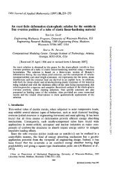
Dynamic response of finite sized elastic runways subjected to ...

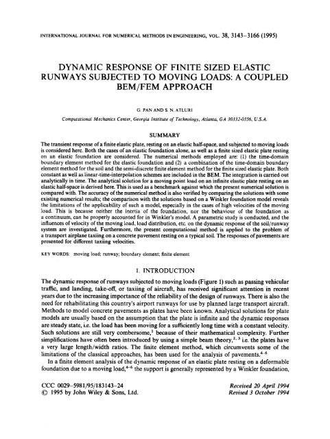
INTERNATIONAL JOURNAL FOR NUMERICAL METHODS IN ENGINEERING, VOL. 38, 3143-3 166 (1995)
DYNAMIC RESPONSE OF FINITE SIZED ELASTIC
RUNWAYS SUBJECTED TO MOVING LOADS: A COUPLED
BEM/FEM APPROACH
G. PAN AND S. N. ATLURI
Computational Mechanics Center, Georgia Institute of Technology, Atlanta, GA 30332-0356, U.S.A.
SUMMARY
The transient response of a finite elastic plate, resting on an elastic half-space, and subjected to moving loads
is considered here. Both the cases of an elastic foundation alone, as well as a finite sized elastic plate resting
on an elastic foundation are considered. The numerical methods employed are: (1) the time-domain
boundary element method for the elastic foundation and (2) a combination of the time-domain boundary
element method for the soil and the semi-discrete finite element method for the finite sized elastic plate. Both
constant as well as linear-time-interpolation schemes are included in the BEM. The integration is carried out
analytically in time. The analytical solution for a moving point load on an infinite elastic plate resting on an
elastic half-space is derived here. This is used as a benchmark against which the present numerical solution is
compared with. The accuracy of the numerical method is also verified by comparing the solutions with some
existing numerical results; the comparison with the solutions based on a Winkler foundation model reveals
the limitations of the applicability of such a model, especially in the cases of high velocities of the moving
load. This is because neither the inertia of the foundation, nor the behaviour of the foundation as
a continuum, can be properly accounted for in Winkler’s model. A parametric study is conducted, and the
influences of velocity of the moving load, load distribution, etc. on the dynamic response of the soil/runway
system are investigated. Furthermore, the present computational method is applied to the problem of
a transport airplane taxiing on a concrete pavement resting on a typical soil. The responses of pavements are
presented for different taxiing velocities.
KEY WORDS: moving load; runway; boundary element; finite element
1. INTRODUCTION
The dynamic response of runways subjected to moving loads (Figure 1) such as passing vehicular
traffic, and landing, take-off, or taxiing of aircraft, has received significant attention in recent
years due to the increasing importance of the reliability of the design of runways. There is also the
need for rehabilitating this country’s airport runways for use by planned large transport aircraft.
Methods to model concrete pavements as plates have been known. Analytical solutions for plate
models are usually based on the assumption that the plate is infinite and the dynamic responses
are steady state, i.e. the load has been moving for a sufficiently long time with a constant velocity.
Such solutions are still very combersome,’ because of their mathematical complexity. Further
simplifications have often been introduced by using a simple beam theory,’. i.e. the plates have
a very large length/width ratios. The finite element method, which circumvents some of the
limitations of the classical approaches, has been used for the analysis of pavement^.^-^
In a finite element analysis of the dynamic response of an elastic plate resting on a deformable
foundation due to a moving load,’-6 the support is generally represented by a Winkler foundation,
CCC 0029-5981/95/183143-24
0 1995 by John Wiley & Sons, Ltd.
Received 20 April 1994
Revised 3 October 1994

3144 G. PAN AND S. N. ATLURI
Pavement (Plate): E, vp pp
Soil (Elastic Space)
E* v, P.
Figure 1. The problem of a moving-load on a runway/soil system
i.e. a set of parallel springs. The Winkler foundation, however, has obvious deficiencies. The
inertia of the foundation,. the continuity and interaction effects within the foundation cannot be
included properly. Since the foundation is, strictly speaking, a continuum, the Winkler foundation
is applicable only for the cases where the foundation is a thin and light layer resting on a rigid
support. In such a case, the inertia, the continuity and interaction effects in the foundation as
a continuum may be neglected. In engineering practice, however, this is not always the case and
these factors may dominate the response of the pavement.
The finite element method can also model the foundation as a portion of a continuum half
space. But the method cannot model the entire half-space: firstly, because a tremendous number
of elements must be used, and secondly, no matter how many elements are used, the infinite
half-space has to be truncated, i.e. an artificial boundary is imposed on the half-space, resulting in
improper satisfaction of the radiation boundary conditions.
On the other hand, the boundary element method, that is used in the present study for the
elastic half-space (which models the soil), requires only a discretization of the contact surface
between the soil and the pavement and automatically accounts for the radiation condition. FEM
can be used for the elastic pavement, with an appropriate choice of finite elements to model the
pavement as a 3-D structure of a finite size. Also, the general time-domain formulation'^* of
BEM, which is a step by step method, has the advantage over frequency-domain form~lation,~ of
leading directly to the time history of the dynamic response and of creating a basis for extension
to non-linear problem.
In this paper, a general purpose method is developed to analyse the dynamic response of an
elastic, finite sized pavement, which rests on an elastic half-space, and is subjected to a moving
load. In the analysis of an elastic foundation subjected to moving loads, two time-marching
schemes are proposed to model the movement of the load. Both the full space Stokes’ fundamental
solution and the half-space fundamental solution are included in the computer code. An
analytical solution for a moving point load on an infinite elastic plate resting on a continuous

FINITE SIZED ELASTIC RUNWAYS 3145
elastic half-space is deduced to be used as a benchmark solution. Then, extensive analyses for
finite plate-soil system are performed numerically, based on the developed soil-structure interaction
analysis methodology for moving loads.
The contents of the paper are as follows. The time-domain boundary element method for an
elastic half-space is developed in Section 2. The computer simulation of responses of the elastic
half-space alone, due to moving loads, is demonstrated in Section 3. The coupled formulation for
an infinite soil (modeled by BEM) pavement (modeled by FEM) interaction under moving loads
is established in Section 4. Section 5 presents an analytical solution for a moving point-load on an
infinite elastic piate resting on an elastic half-space. The responses of a finite sized elastic
pavement resting on an elastic half-space, and subjected to moving loads, are investigated in
Section 6. An aircraft taxiing problem is solved and discussion in Section 7. Conclusions are given
in Section 8.
2. TIME-DOMAIN BOUNDARY ELEMENT FORMULATION FOR THE
RESPONSE OF AN ELASTIC HALF-SPACE (MODEL FOR THE SOIL) SUBJECTED TO
A MOVING LOAD
In this section, a dynamic boundary element formulation for an elastic half-space (soil without the
pavement) is presented. The numerical implementations are described for both the cases where
the full-space and the half-space fundamental solutions are used. Furthermore, time marching
schemes for moving load problems are described and are discussed.
The governing equations, in terms of displacements, for a homogeneous isotropic linear elastic
solid can be written as
(c: - c:)u~, ij + ~3.j. ii + (bj/p) = iij (1)
where bj is the body force, ui are Cartesian displacement components, and
c: = (L+2P) -P
~
7 cz--
P
P
where I and p are Lame’s constants, p is the density of the solid.
The stresses and displacements should satisfy the following boundary conditions:
t(n)i(X, t ) = pi(x, t),
ui(x, t ) = qi(X, t),
x E Bt
x E Bu
where B, is the traction prescribed boundary; B, is the displacement prescribed boundary; and
B = B, + B, and the initial conditions are:
Ui(X, O+) = UOi(X), tii(X, O+) = UOi(X) (4)
Consider two distinct elastodynamic states, one being [u, t] and the other [u’, t’] (where bold
letters denote vectors), with the initial condition,
From the dynamic reciprocal theorem, we have:
Ui(X, O+) = u&(x), tif(x, O+) = &(x) (5)
r P P P
J t*u’dB + J p{b*u’ + vou’ + uou’} dV = J t’*udB + J p{b*u + vbu + ubu} dV (6)
dD D JD D
(3)

3146 G. PAN AND S. N. ATLURI
where b is the body force for the [u’, t‘] state, and 4*$ is the convolution integral that is defined
by:
J-;
C4*IC/l(X, t) = 4b, t - T)IC/(X, T)dT (7)
[u’, t’] is chosen to be the state corresponding to a unit impulse at < in the direction of xk axis in
the infinite media, i.e.
pb = s(t)s(x -

FINITE SIZED ELASTIC RUNWAYS 3147
0
(a)
Figure 2. (a)Arbitrarily distributed load q(& q) moving at speed u(r); (b) the loading history at a spatial point (x, y),
assumed to be constant in the time interval < 7 < T , on ~ an arbitrarily shaped spatial-patch
where
7,1 =
xo, - x - a1(y)
4)
9 7r2 =
The load history at point (x, y) can be expressed as
(b)
XO’ - c + az(Y)
c(t)
ts3(~7 Y, T) = 4(t)CH(t - trl) - H(T - ~ r2)l
where ts3 is the vertical surface traction (i.e. normal to the half-space surface) applied on the
half-space.
The Stokes’ displacement solution for an impulse load 6(t - T )~(x -

3 148
for i = 1,2
G. PAN AND S. N. ATLURI
r
q if-

FINITE SIZED ELASTIC RUNWAYS 3149
The numerical results using the Green's function for a half-space are in good agreement with
analytical solutions. While the analytical solutions are for the infinitely long (w --* 00) strip load
that moves from infinity to infinity, and whereas in the present BEM analysis, W and L are of
finite size, the differences between the two solutions are still small. The difference will be further
lessened as Wand L increase. This tendency will also be shown in Section 3.2. Similar agreement
with analytical solutions for the case when the load moves at transonic speeds (c = 300 m/s) as
well as supersonic speeds (c = 600 m/s) is achieved.
3.2. The Efects of W(Length of the Moving Strip Load) and of C (the Moving-Load-Velocity) on
the Dynamic Response
The boundary element method for the moving load problem, unlike the analytical ~olution,'~ is
applicable for an arbitrary moving speed (including accelerating/decelerating loads) and for an
arbitrary spatial distribution of the load. In this section, we present some characteristic responses
of the soil due to moving loads, the corresponding solutions for which cannot be obtained using
the existing analytical ~olution'~ method. The parameters used are the same as those previously
employed, unless otherwise indicated.
The deflections of the ground surface as W increases, for a speed u = 300 m/s, are shown in
Figure 4. The curves represent the deflections, for W= 2.5, 10 and 40m, respectively
(L = 18.75 m). The deflection behind the moving load recovers slower for larger W than it does
for smaller W. The pit behind the moving load extends further and further as W increases and
eventually it will extend to infinity as W increases to infinity.
The typical time history of deflection at the center of surface of the ground as the load
moves from right to left for 2b x 2 W = 0-625 x 2 x 20 m2 and c = 200 and 300 m/s are shown in
Figure 5 and are compared to the static solution. The distance passed by the moving load is
from - 60 x (26) to 60 x 2b. The deflections in subsonic case c = 200 m/s are almost
symmetrical, similar to that in static case. But the maximum deflection is remarkably larger
than that in static case. Also, the surface of the ground has some upward deflection. In the
supersonic case (c = 300 m/s), the deflections of the ground surface before the load are
zero (undeformed) while those behind it form a pit tail extending further than those in transonic
case.
0.01 '
l m
position of the load dong x-axii
Figure 4. Deflection at (x = 0, y = 0) for various locations along the x-axis of the moving load (of width 26 in the
x direction and length 2 W along the y direction) for the transonic case (c = 300 m/s): the effect of changing values for
W(Note: load travels from x = - L) w = 2S(-), w = lo(------), w = 40( .......)

3150 G. PAN AND S. N. ATLURI
Figure 5. Deflection at (x = 0, y = 0) for various locations along the x-axis of the moving load (of width 26 in the
x direction and length 2W along the y direction) for the transonic case (c = 300 m/s): the effect of moving-load velocity
(Note: load travels from x = - L) c = l(static) (-), 200------), 300 m/s(. . . . . .)
4. TIME DOMAIN FORMULATION FOR THE PROBLEM OF THE RESPONSE
OF THE SOIL (BY BOUNDARY ELEMENTS)-RUNWAY (BY FINITE ELEMENTS)
SYSTEM TO A MOVING LOAD
In establishing the formulation of the interaction problem, a frictionless interface is asumed to
exist between the pavement and the half-space, since the effect of shear stresses at the interface on
the vertical displacement is known to be small.'' The only non-zero components of Tik in
equation (12) are T13, TZ3, T31 and T32, coupling the vertical and the horizontal motions. The
horizontal motion of the soil is negligible, hence the second term on the right-hand side of
equation (12) vanishes.
Thus, from equation (12), for k = 3, the vertical displacement us3 at any time t and position on
the surface B of the soil medium can be expressed as
where ts3 are the vertical surface tractions applied on the contact region between the pavement
and the foundation. For simplicity, but without loss of generality, perennial contact between the
pavement and the soil is assumed in the present work.
The integral equation (17) can be discretized (i) by dividing the contact region with M rectangular
elements, and assuming a constant distribution of contact tractions and displacements over
each element, and (ii) by dividing the time interval (0, t) into N number of time steps with
a constant or linear time variation of tractions and displacements during each time step. Thus,
equation (17) can be reduced to the following set of algebraic equations
1 N M
where q is the time step at which loads begin to apply. UtjR is the vertical displacement of the
element R (receiver) at time step N, tfj" is the vertical traction applied on the element S (source) at
time step 1 and G2; is the discretized Stokes' solution.
Equation (18) can be written for all the M elements, in a matrix form as
f {&} = [c:~] {tf33) + {RTN) (19)

FINITE SIZED ELASTIC RUNWAYS 3151
where the M x M influence matrix [GG] expresses the vertical displacement during the Nth time
step due to unit surface vertical tractions applied during the same time interval. {RTN} is shown
to be:
n=q+l
It should be noted that the vector {RTN} can be considered to be known during each time step,
since it only involves quantities computed in the previous time steps.
The dynamic equation for the plate12 can be written as
[MI{& + CKI{dl = {P(O} + {R) (21)
where {d} = {ur3, Ox, O,} (transverse displacements and their derivatives), p(5) is the moving load
at position (, {R} is the nodal vertical contact force vector.
Using the Newmark-/? time-domain discretization scheme,l3 equation (21) can be written as
where
([Kl + ao[Ml){dN} = {pN(5)} + {RN} + [M](ao{dN-’} + al{dN-’} + a22{aN-1}) (22)
1
a. = -
W)”
1 1 1
/-?(At)’ 28 4
a, =- a2 = - - 1, 8 = -(05 + a)’, a = 0 5
After condensation to eliminate rotational degrees of freedom, equation (22) can be reduced to:
[KC]{&) = {P”> + {RN) + {QN} (23)
where [Kc] is the total stiffness matrix, {p”} is the moving load vector, {QN} is the inertia force of
the plate, and {RN} is the nodal vertical contact force vector when load is at position cN:
{RN) = [A] {ty3} (24)
where [A] is the diagonal matrix whose element Aii represents the area of element i,
i = 1, 2, ... , M, {tY3} is the vertical surface traction applied to the plate.
For the soil-foundation system (Figure 4), the displacement compatibility can be written as
The traction equilibrium can also be written as
{$3l = {.:3> (25)
{tY3> = - (tsN33)
Eliminating {tr3} from equations (19), (23) and (24), one obtains:
Equation (27) is the finite element-boundary element coupled system of equations for the
response of the soil-pavement combination.
It should be noted that, in equation (27), the diagonal terms of [Gi3} are the integrals of
singular kernel function during the first time interval over each element when the source point is
inside it. A special care must be taken for such singular integrals. Since constant tractions and
displacements over each element is assumed, the singular integrals can be evaluated analytically
for both constant and linear time variation of tractions and displacements. The analytical
formmula for singular integrals will be given below.

3152 G. PAN AND S. N. ATLURI
In the case of linear time interpolation, a variablef(x, t) (some quantity at location x and at
time t), can be expressed in terms offj(x), wherefj(x) is the discrete values off(x, t) at the end of
jth time step as’
N
f(x, 7) = c CM;f”-’(x) + M”F(x)l (28)
n= 1
where
where $,,(T) = 1 for (n - 1)At < I zn At, and = 0 otherwise.
During the first time interval
When zero initial conditions are assumed, the first term on the right-hand side of (30) is zero.
For the kernel function as expressed in (14) and f(x, z) = ts3(x, T), the above integral can be
written as
where
r
= -L[(C---“)H(At-
r 2 3At
7
I6(At - 7 - Ar)-41(z)dIdz +
At
1
I(At - h)- $](At - h)dI +
At
cir At
J.r)]:::I+LL(At-i)H(At-k)
c;r r
0 if At < -
c1
--z-(~--) 3c:At if C1
[(g-&)H(At-Ar)] (At)2 1 (At)’ r r r
-

FINITE SIZED ELASTIC RUNWAYS 3153
5. ANALYTICAL SOLUTION FOR A ‘MOVING POINT-LOAD ON AN
INFINITE ELASTIC PLATE RESTING ON AN ELASTIC HALF-SPACE
This solution will be used as a benchmark against which the numerical results obtained by the
present BEM are compared. Here the plate is idealized to be an infinite elastic plate resting on an
elastic half-space. A unit load moves along the x axis, from the negative infinity to the positive
infinity in the x-y plane, with a uniform speed c. The deflection of the plate is governed by
where w(x, y) is the transverse deflection, p(x, y) is the contact pressure between the plate and the
foundation, D is the rigidity of the plate, p’ is the mass of the plate per unit area.
On the other hand, the system of equations describing the motion of the foundation is written
as
where
ao
(A + G)- + GV’U = c2p-
ax
ao
aY
ao
aZ
a2u
ax2
a2v
(A + G) - + GV’U = c2p 2
(A + G)-+ GV’W = c2p-
au ay aw
@=- +-+ax
ay aZ
u, u and w are deflections of a point in the soil, along the x, y and z direction, respectively.
The boundary conditions for z = 0 are expressed by
a*w
ax2
(34)
6, = - P(X, Y), Txr = 0, zYz = 0 (35)
The solution of equation (34) can be expressed, using functions f and gi (i = 1,2,3) as
u=-
af
a!
af
ax aY az
+g1, u=-+g2, w=-+g3
Substihting the expression (36) in (34), it is found that function f and gi must satisfy:
where al = c/c,, at = c/c2.
Equations (33) and (37) can be solved by the method of two-dimensional Fourier integral
transformation,
f.e-f(xql+YqZ)dXdy f-
F. ei(xqi +YQZ)dq
1 dqz (38)

3154 G. PAN AND S. N. ATLURI
After the Fourier transformation, we have the equation for the plate as
w?': + 24:q: + 4:) W(41 9 qz) - m'c2d W(q1, qz) + P(q19 42) = 1 (39)
and from equation (37) for the half-space,
($-n:)F=O (-$-n;)Gi=O, i = 1,2,3
where n: = (1 - a:)q: + q:, n: = (1 - a:)q: + 4:.
If the subsonic speed case, i.e. c < cz < cl, ni' > 0, i = 1,2, is considered here (the other cases
are omitted here for brevity), the solution of (40) may be assumed to be in the form
F = A4e-"t2
Gi = Aie-"2z, i = 1,2,3 (41)
By using this expression, the boundary conditions (35) and the governing equation (40) can be
written as
- &A3 + (4: + q: + n:) = - P/G, - nzAl + iqlA3 - 2iqlnlA4 = 0
- nzAz + iqzA3 - 2iqznlA4 = 0, qlA1 + qzAz + inzA3 = 0
From (36) and (39), we can express P as
Wq1, qz)L=o = A4( - nl) + A3
P = 1 - [D(q: + 2qfqZ + q 3 - p'c2q:1( - nlA4 + A3)
Substituting equation (43) in (42), a system of algebraic equations, from which Al, Az, A3 and A4
can be solved, is obtained. Thus, expressions for Al , Az, A3 and A4 are obtained and are written
as
P 2iqlnlnz P 2iqznlnz
A1 =G
B 9 AZ=G B
(44)
A - __
P 2nl(4: + 42) P 4: + q: + n:
3-
G B , A4=7j B
where,
B = (4: + 4: + n: + c/G)(qy + q: + n:) - (2nz + c/G)2ni(q: + 4:)
Substituting (44) in (43), after inverse transformation, we have
(42)
(43)
or omitting the imaginary part,
Transforming the coordinate system to the cylindrical one, we obtain the final expression,
Jm cosZ 8 cos(r(x cos 8 + y sin 0))dr d8
B
(46)

FINITE SIZED ELASTIC RUNWAYS 3155
where
- (2 ,/- + r/G(DrZ - p'c2 cos2 8 ) ) 2 J m
where 8 = n/2, the integrand is singular and should be replaced by 1/(2(a: - af) - r/GDr2a:)
6. DYNAMIC RESPONSE OF AN ELASTIC PAVEMENT RESTING ON AN
ELASTIC FOUNDATION, DUE TO A MOVING LOAD
6.1. Comparison with Static Solution
The static deflection of a uniformly loaded square elastic plate, which rests on an isotropic
elastic half space are presented in Figure 6. The uniform load density is 1. The present BEM
solution is compared to that of Cheung and Zienkiewicz. lS The contact pressure variation along
the centre line of the plate is given for stiffness y = 180n(E,/E,)(~/t)~ = 1, where E, is the Young's
modulus of the soil, E, is the Young's modulus of the plate, a is one-twelfth of the length of the
edge of the square plate and t is the thickness of the plate.
The plate elements used in this work are 12-degree-of-freedom rectangular elements (Rl). The
mesh consists of 20 x 20 finite elements, 21 x 21 boundary elemens (constant elements), with
10 x 10 subelements (for accuracy purpose, every boundary element is divided into a number of
subelements, so that the contribution from any wave source point to this boundary element can
be obtained more accurately by summing up the contributions to all its subelements). The present
results agree well with those in Reference 15 (in Reference 15, 6 x 6 constant rectangular finite
elements, i.e. they are assumed to be uniformly loaded, were used for the plate and Boussinesq
equation was used to model the half-space). The results corresponding to the Winkler foundation
are also plotted as a flat horizontal line. It is seen that the solution of uniform contact traction
between plate and soil by Winkler's model is a very rough approximation.
C
.-
0
c
0
c z
3
w
0
m
c
C 0
0 2
R - ~
-
5 1
present solution
Winkler's solution
-
1
- I
0 1 2' 3'
distance from center line
Figure 6. Contact traction under a uniformly distributed static loaded square plate[ - 3a d x < 3a, - 3a < y d 3a]

3156 G. PAN AND S. N. ATLURI
6.2. Response to Stationary Harmonic Force
In order to verify the FEM-BEM methodology developed in the present study, the vertical
response of a square elastic plate, resting on an elastic half-space, subjected to a uniformly
distributed harmonic vertical load is analyzed. The amplitude of vertical displacement at the
centre of the plate versus the frequency s given in Figure 7 and is compared to that in Reference
16. Also, the vertical motions of the three points (centre point, mid-point of the edge and the
corner point) are also plotted versus time in Figure 8(a), (b) for w = 9150 and w = 18 300,
respectively. The parameters used are, plate dimensions: 60 x 60 x 11517 in, plate properties:
E, = 30.004 x lo6 psi, vp = 0.3, pp = 7-34 x lb-s2/in4; and soil properties: E, = 8.84 x lo6
psi, v, = 0.3, ps = 2.82 x lb-s2/in4 .4 x 4 finite elements and 5 x 5 boundary elements, with
5 x 5 subelements are used here.
6.3. Moving Line Load Problem
The numerical solution for a large thin plate resting on an elastic half-space is compared to the
exact solution for an infinitely large plate resting on an elastit half-space, and subjected to line
load that is infinitely long in the y direction and moving along the x direction'. The geometry and
material properties are, plate dimensions: 120 x 60 x 5 in., plate properties: E, = 1.6 x lo6 psi,
\I, = 0.25, pp = 2-88 x lb-s2/in4; and soil properties: E, = 0.2 x lo6 psi, v, = 0.25, ps =
2.0 x lb-s 2/in4 (c2 = 2000 in/s).
In Reference 1, an infinite plate is subjected to a line load that moves with constant velocity.
The transient motion becomes negligible after some time and the motion will approach steady
state. In the pesent finite element-boundary element analysis, it is difficult to obtain the steadystate
response since the infinite plate is represented by a finite plate. However, the effect
of transient motion can be reduced if a considerably large plate is assumed. Here a plate that can
be analysed within the capacity of an engineering work station is considered. 24 x 12 finite
elements and 25 x 13 boundary elements with subelements 5 x 5 are used in the numerical
calculation.
Figure 9 displays the variation of the bending moment in the plate, when the moving line load
is at x = 0 for different rigidity values of the plate G,/G, = 8,40,80 (where G, and G, are the shear
moduli of the plate and soil, respectively). Small discrepancies are observed between the solutions
of present method and the analytical solutions because the model that is used in the numerical
3.5
4r
3,
2.5 '
2
I. 5
1,.
0.5t
amplitude(in x lo4)
60
Figure 7. Vertical displacement at (x = 0, y = 0) of a square plate ( - 30 Q x, y C 30) which is subjected to a uniformly
distributed harmonically varying vertical load: effect of harmonic frequency (comparison of present result with those in
Reference 16). (-) solution in Reference 16, (......) present solution

FINITE SIZED ELASTIC RUNWAYS 3157
0.
0.
Figure 8(a) Vertical displacement at (x = 0, y = 0); (x = 30, y = 0) and (x = 30, y = 30) of a square plate
( - 30 < x, y < 30) which is subjected to a uniformly distributed harmonically varying vertical load (for o = 9150).
(b) Vertical displacement at (x = 0, y = 0); (x = 30, y = 0) and (x = 30, y = 30) of a square plate ( - 30 < x, y < 30)
which is subjected to a uniformly distributed harmonically varying vertical load (for o = 18 300)
analysis does not represent the exact steady-state response and therefore includes some transient
responses in the solution.
The results are also compared to the corresponding bending moment in an infinite plate resting
on Winkler foundation. Following Biot,” the modulus of the foundation k is calculated by
equating the bending moments under a stationary load for a plate on a Winkler foundation to
those on a continuous foundation (k = 14000 is thus obtained). The comparisons are shown in
Figure 10(a) and (b) for two different velocities c/cz = 0.3 and 0.7, respectively (c2 is the shear
wave speed of the ground medium). For a relatively low moving-load velocity, the discrepancies
in the bending moment as functions of r/h, are small, as shown in Figure 10(a). But the
discrepancies increase at high velocities, as shown in Figure lO(b). This reveals that the modulus
of the foundation k, which is obtained from static equivalence, does not give good predictions for
the moving load problem, especially for high moving load velocity problems. In other words, the
modulus for the foundation k in Winkler’s model should be different for different moving load
velocities. This suggests that k be no longer a material parameter for the pavement, but
a parameter which depends on the moving load velocity.
The results for the contact pressure between the plate and foundation are shown in Figure 11 (a)
and (b) for c/cz = 0-3 and 0.7. The comparisons reveal that the results of Winkler’s model deviate
from those of continuous model, particularly in the vicinity of the load point, and that the
solutions of the present scheme converge to the infinite plate analytical solutions.’ This reveals

3158 G. PAN AND S. N. ATLURI
h
?!
r
U
Y
.
z
Achenbach Gp/Gs=8
--*- present Gp/Gs=8
--.&--
Achenbach Gp/Gs=4O
present Gp/Gs=40
Achenbach Gp/Gs=80
--*- present Gp/Gs=80
0-
-1
0 2 4 6 8
r/( h/2)
Figure 9. The bending moment in the plate versus r/(h/2) (for the case c/c2 = 0.3 and Gp/Gs = 8,40,80) in the problem of
an infinite elastic plate resting on an infinite elastic half-space, subjected to a infinite long (along the y direction) moving
line load
that the modulus of the foundation k, which is obtained from the static bending moment
equivalence, does not give good prediction for the contact pressure.
It is noted that the present finite element-boundary element approach gives good estimations
for the quantities (bending moment, contact pressure, etc.), especially at the vicinity of the
load point, despite the influence of the transient response inevitably included in the numerical
results.
6.4. Moving Point Load Problem
The numerical solution for a moving point load on a large plate resting on an elastic half-space,
is compared to the analytical of an infinitely large plate resting on an elastic half-space that is
derived in Section 4. All the parameters are the same as those in Section 6.3. The analytical
solution using Winkler’s model is also given. The modulus of the foundation k is calculated by
equating the maximum displacement under a static load (k = 8200 is thus obtained). Figure 12
reveals the apparent discrepancy between the analytical solution using elastic half-space and that
using Winkler foundation. Figure 13(a) and (b) for c = 0 and c/cz = 0.5 show that the numerical
solutions of present BEM-FEM approach converge to the analytical solutions of continuous
foundation. But the solutions of Winkler’s model differ from them, especially at those points that
are at some distance from the load point.

FINITE SIZED ELASTIC RUNWAYS 3159
- Achenbach
---o-- present
.................. Winkler's model
-0.4 1
2 4 6
r/(h/>
21
.
I
- Achenbach
--*-- present
..--
Winklet's model
(b)
.1
0 2 4 6 8
rl(hi2)
Figure 10. (a) The bending moment in the plate versus (r/(h/2)(for the case c/c2 = 0.3 and Gp/Gs = 8) in the problem of
an infinite elastic plate resting on an infinite elastic half-space, subjected to a infinite long (along the y direction) moving
line load. Comparison of present numerical solutions with those by using Winkler's model and those by using analytical
method in Reference l.(b) The bending moment in the plate versus r/(h/2) (for the case c/c2 = 0.7 and Gp/Gs = 8) in the
problem of an infinite elastic plate resting on an infinite elastic half-space, subjected to a infinite long (along the
y direction) moving line load. Comparison of present numerical solutions with those by using Winkler's model and those
by using analytical method in Reference 1.
6.5. Parametric Study with Varying Moving-Load Velocity
The behaviour of an elastic pavement resting on an elastic half-space for different moving load
velocities is studied. The geometry and material properties are plate dimensions: 300 x 12 x 3 in;
plate properties: E, = 3.0 x lo5 psi, v, = 025, pp = 2.0 x lb-sz/in4; and soil properties:
E, = 1.8288 x lo3 psi,v, = 0.4, p, = 1.5 x lb-s2/in4 (c2 = 2086 in/s). The concentrated moving
load is 4 x lo3 kips. The variation of maximum deflection with increasing velocity of moving
load is presented in Figure 14. For low moving load velocity (CL700 in/s), the maximum deflection

0'02 1
---
Achenbach
0-- present
.
Winkler's model
(a>
-0.08
0
1 I 1
2 4 6 8
r/( h12)
---O--
.
Achenbach
present
Winkler's model
Figure 11. (a) The contact traction under the plate versus r/(h/2) (for the case c/c2 = 0.3 and Gp/Gs = 8) in the problem
of an infinite elastic plate testing on an infinite elastic half-space, subjected to a infinite long (along they direction) moving
line load. Comparison of present numerical solutions with those by using Winkler's model and those by using analytical
Reference method in 1. (b) The contact traction under the plate versus r/(h/2) (for the case c/c2 = 0.7 and Gp/Gs = 8) in
the problem of an infinite elastic plate resting on an infinite elastic half-space, subjected to a infinite long (along the
y direction) moving line load. Comparison of present numerical solutions with those by using Winkler's model and those
by using analytical method in Reference 1.

FINITE SIZED ELASTIC RUNWAYS 3161
of the plate is about the same as in the static solution, but, for the speed above 700in/s, it
increases with the speed. It is observed that there is a peak at the velocity of 2200 in/s, which is
about the speed of the Rayleigh wave propagating along the surface of the soil. The plate is long
enough that the solution almost approaches its steady state solution. Therefore, at the vicinity of the
area where the moving load is applied, the displacements and contact pressures between the plate
and the soil keep almost unchanged and also move along with the moving load at the speed of c.
3 OOe-7 -/ I
0.0 0.2 0.4 0.6 0.8 10
cic2
Figure 12. The deflection under the moving point-load versus and load velocity in the problem of an infinite elastic plate
resting on an infinite elastic half-space, subjected to a moving point-load. Comparison of present analytical solutions
(presented in Section 5) with those by using Winkler’s model.
4’00e-71 Deflection (in,
1 - present analytical solution
. - ....
Winkler’s solution
present numerical solution
2.00e-7 -
1.00e-7 -
0 2 4 6 fi
r/(h/2)
(4
Figure 13. (a) The deflection distribution of a plate along the centre line of y direction versus r/(h/2) (for the case
c/c2 = 0.) in the problem of an infinite elastic plate resting on an infinite elastic half-space, subjected to a moving
point-load. Comparison of present numerical solution with those by using Winkler’s model and those by using analytical
methods in Reference 1. (b) The deflection distribution of a plate along the centre line of y direction versus r/(h/2) (for the
case c/c2 = 05) in the problem of an infinite elastic plate resting on an infinite elastic half-space, subjected to a moving
point-load. Comparison of present numerical solution with those by using Winkler’s model and those by using analytical
method in Reference 1.

3162
G. PAN AND S. N. ATLURI
4'00e-71 Deflection (in)
'. -.
'. -.
. .
1 ......
0.14,.
0.12.
0.1;
0.08.
0.06.
0. 04-
0.02.
Figure 14. Maximum deflection at the plate centre in the whole history of a load moving through a plate versus
load-moving-velocity in the problem of an finite-sized elastic plate resting on an infinite elastic half-space, subjected to
a moving point-load
The deflection distributions of the plate due to the load, moving in the positive X direction, are
shown in Figure 15 for c = 1000,2000,6000 in/s, respectively. This result shows that in the low
velocity case, symmetry is exhibited in the deflection distribution. But as the moving-velocity
increases, the unsymmetry takes over and it becomes more and more pronounced.
The time history of deflection of another plate whose size is 1 x b = 120 x 60 in2 for
c = 500, 5000 in/s at the transmit time t/T = 0,0.2,0.4,06,0.8 and t/T = 0,02,0~4,0-6,0-8, 1.0
(where T is the time needed for the moving load to travel across the plate) is shown in Figure
16(a), (b) from left to right, respectively. Figure 16(a) shows the result of the low velocity case
c = 500 in/s. There is almost no upward deflection. The static deflection due to the load plays
a dominant role.
The case of relatively high velocity c = 5000 in/s is illustrated in Figure 16(b). It is observed
that the point of maximum transverse displacements is always behind the load and it proceeds in
a wave-like manner. Unlike that in the low velocity case, the plate exhibits an upward deflection.

FINITE SIZED ELASTIC RUNWAYS 3163
0.02-
-0.04..
-0.06.
-0.08-
-0.1-
-0.12-
-0.14-
Figure 15. Deflection distributions of a plate along the x direction (moving direction) in the problem of an finite-sized
elastic plate resting on an infinite elastic half-space, subjected to a moving point-load for the case of c = IOOO(. . . . .),
2200(-), 6OOO(------) in/s
0.021 psition in the plate (x 150 in)
-0.121 c
-0.14
3
0.021 position in the plate (x 150 in)
Figure 16. (a) Deflection distributions of a plate along the x direction (moving direction) in the problem of an finite-sized
elastic plate resting on an infinite elastic half-space, subjected to a moving point load for the case of c = 500 in/s and at the
moments of t/T= 00, 0.2, 0.4, 0.6 and 0.8 (where T is the time needed for the load to travel through the plate).
(b) Deflection distributions of a plate along the x direction (moving direction) in the problem of an finite-sized elastic
plate resting on an infinite elastic half-space, subjected to a moving point load for the case of c = 5000 in/s and at the
moments of t/T = @0,02,0.4,06 and 0.8 (where T is the time needed for the load to travel through the plate)

3164 G. PAN AND S. N. ATLURI
7. THE PROBLEM OF TAXING OF AN AIRPLANE ON AN ELASTIC RUNWAY
RESTING ON AN ELASTIC HALF-SPACE
The present methodology is applied to obtain the response of the pavement, while a B-747-200B
aircraft is taxiing. The taxiing speed of the airplane is varied within a range (50-150 m/s). The
following are typical values for the material properties and the dimensions of the aircraft-pavement
system.
Pavement properties: slab width = 7.62 m (300 in), length = 22.86 m (900 in), thickness = 0305 m
(12 in); E, = 2.5 x 10" kg/m2 (3.6 x lo6 psi), vp = 015, pp = 2.32 x lo3 kg/m3 (0.0002174 lb-~~/m~)~';
I Y
olo
I
-----_
r-----
olo
I
X
Gear Load = 178.57 kips
Wheel Load = 44.64 kips
Gear No. 2
Wheels = 4
CoordWheell
X(inches)
Y(inches)
1 I 2 I 3 I 4 I
-25.0 -25.0 25.0 25.0
-20.0 20.0 -20.0 20.0
Figure 17 Aircraft B-747-200B and gear confiwration with five gears (four wheels in each of four rear gears and two wheels in
the front gear). Response calculated for four wheel loads of one rear gear (gear No. 2)

FINITE SIZED ELASTIC RUNWAYS 3165
0.001
2.5335
-
i -0.0005
0
-0,001
-0.0015
-0.002
I I I I I 1 I
distance (x25 in)
position in thc pkte (x25 in)
Figure 18. The deflection distributions of a concrete pavement for the cases of o = SO, 100,150 m/s and at the moment of the
gear position being at the centre of the plate in the problem of an B-747-200B aircraft taxiing on a concrete pavement resting on
a typical soil. Response calculated for four wheel loads of one rear gear (gear No. 2)
Soil propertities: E, = 2.0 x 10' kg/m2, v, = 0.40, p, = 1.5 x lo3 kg/m3; aircraft properties: gear load
is 4 x 202 487 N (4 x 44.64 kips), wheel spacing is 40 in (in the moving direction) x 50 in.
The aircraft and gear configuration used are both shown in Figure 17(a) and (b). The effect of
the moving speed on the deflection distribution along the centre line when the moving load is at
the centre of the plate is shown in Figure 18 for D = 50,100,150 m/s. The three curves corresponding
to the three speeds show the influence of the moving speed. As the moving speed
increases, not only the deflection itself, but also its gradient increases around the load applied
area. In the high speed case, the deflection assumes an unsymmetrical distribution and the
deflection behind the moving load is larger than that in front of the load.
8. CONCLUSIONS
In this paper, a boundary element approach and a finite element-boundary element coupled
approach are presented to analyse the dynamic response of elastic half-space alone and that of an
elastic runway resting on an elastic half-space, respectively, due to moving loads. Numerical
analyses are carried out to study the dynamic response of pavements. The numerical results show
good agreement with the analytical solutions based on continuous foundation model, but differ
from those based on discrete Winkler's model. The discrepancies depend on the load types, the
velocities of the moving load, the sizes and properties of the plate and foundation, the unknown
variables, etc. The results reveal the limitations of Winkler's model in pavement response analysis,
especially in the cases of the high moving-load velocity.
A parametric study is also conducted to study the effects of various parameters on the dynamic
response of an elastic half-space alone, and that of an elastic plate resting on an elastic half-space
due to moving loads. The results show that not only the maximum values of the displacements

3166 G. PAN AND S. N. ATLURI
but also the displacement distributions change as the moving-load velocities increase. At a certain
moving load velocity, the displacements reach their peak values. The distributions exhibit
remarkable changes with respect to the moving load velocity.
Furthermore, the responses of an elastic runway resting on an elastic half-space, due to
a taxiing B-747-200B airplane are investigated for different taxiing speeds. This investigation
suggests that the taxiing of the airplane at a higher velocity produces a larger deflection as well as
deflection gradient of the pavement. This may then cause an increase of the stresses in the
pavement and influence the fatigue life of the pavement structure.
Compared to the case where finite element method is employed for both the plate and the soil,
the present method has the advantages in modelling the radiation condition and also reduces the
dimensions of the problem by one, since only the contact soil-foundation surface is discretized.
The method presented here can be extended to include multi-soil layer foundation and the
non-linear deformation of soil.’
REFERENCES
1. J. D. Achenbach, S. P. Keshava and G. Herrmann, ‘Moving load on a plate resting on an elastic half space’, J. Appl.
Mech., 35, 910-914 (1967).
2. J. T. Kenney, ‘Steady-state vibrations of beams on elastic foundation for moving load‘, J. Appl. Mech., 21, 359-364
(1954).
3. J. D. Achenbach and C. T. Sun, ‘Moving load on a flexible supported timoshenko beam’, Int. J. Solids Struct., I,
353-370 (1965).
4. M. R Taheri and E. C. Ting, ‘Dynamic response of plate to moving loads: structure impedance method’, Comput.
Struct., 33, 1379-1393 (1990).
5. M. R. Taheri and E. C. Ting, ‘Dynamic response of plate to moving loads: finite element method’, Comput. Struct., 34,
509-521 (1990).
6. M. Zaman, M. R. Taheri and A. Alvappillai, ‘Dynamic response of a thick plate on viscoelastic foundation to moving
load’, Int. J. Numer. Methods. Geomech., 15, 627-647.
7. P. K. Banerjee, S. Ahmad and G. D. Manolis, ‘Transient elastodynamic analysis of three dimensional problem by
boundary element method‘, Earthquake eng. struct. dyn., 14, 933-949 (1986)
8. D. L. Karabalis and D. E. Beskos, ’Dynamic response of 3-D rigid surface foundations by time domain boundary
element method’, Earthquake eng. struct. dyn., 12, 73-93 (1984).
9. S. Kobayashi, ‘Fundamentals of boundary integral equation methods in elastodynamics’, in C. A. Brebbia (ed.) Topics
in Boundary Element Research, Vol. 2, Springer-Verlag, Berlin, New York, (1984). 1-54.
10. T. Triantafyllidis, ‘3-D time domain BEM using half-space Green’s functions’, Eng. Anal. Boundary Elements, 8,
115-124 (1991).
11.
12.
13.
14.
15.
16.
17.
18.
C. L. Pekeris, ‘The seismic surface pulse’, Geophys., 41, 409-480 (1955).
D. J. Dawe, ‘A finite element approach to plate vibration problems’, J. Mech. Eng. Sci., 7(1), 28-32 (1965).
N. M. Newmark, ‘A method of computing for structural dynamics’, ASCEEM3,85, 67-94 (1959).
L. Fryba, Vibration of Solids and Structures Under Moving Load, Noordhoff, Leiden, (1972).
Y. K. Cheung and 0. C. Zienkiwicz, ‘Plates and tanks on elastic foundation’, Int. J. Solids Struct., 1,451-461 (1965).
W. L. Whittaker and P. Christiano, ‘Dynamic response of plate on elastic half space’, ASCE EMl, 108, 133-154
(1 982).
M. A. Biot, ‘Bending of an infinite beam on an elastic foundation’, J. Appl. Mech. Trans. ASME., 59, Al-A7 (1937).
S. Ahmad and P. K. Banerjee, ‘Time domain transient elastodynamic analysis of 3-D solids by BEM, Int. j. numer.
methods eng., 26, 1709-1728 (1988).
19. D. L. Karabalis and D. E. Beskos ‘Dynamic response of 3-D flexible foundations by time domain BEM and FEM’,
Soil Dyn. Earth. Eng., 4, N2, 91-101 (1985).
20. A. B. Kukreti, M. R. Taheri and R. H. Ledesma, ‘Dynamic analysis of rigid pavements with discontinuity’, J.
Trumportation Eng., 118, 341-360 (1992).
21. G. Pan, ‘Dynamic response of pavements under moving loads: boundary element and finite element methods’, Ph. D.
Thesis, Georgia Institute of Technology, Atlanta, GA, (1995).