on the hybrid stress finite element model for incremental analysis of ...
on the hybrid stress finite element model for incremental analysis of ...
on the hybrid stress finite element model for incremental analysis of ...

You also want an ePaper? Increase the reach of your titles
YUMPU automatically turns print PDFs into web optimized ePapers that Google loves.
hr. J. Solids Snuctures. 1973. Vol. 9, pp. 1177 IO 1191. Pergam<strong>on</strong> Press. Printed in Great Britain<br />
ON THE HYBRID STRESS FINITE ELEMENT MODEL FOR<br />
INCREMENTAL ANALYSIS OF LARGE<br />
DEFLECTION PROBLEMS<br />
SATYANADHAM<br />
ATLURI<br />
Department <strong>of</strong> Aer<strong>on</strong>autics and Astr<strong>on</strong>autics,<br />
University <strong>of</strong> Washingt<strong>on</strong>, Seattle, Washingt<strong>on</strong> 98105, U.S.A.<br />
Abatmct-An extensi<strong>on</strong> <strong>of</strong> <strong>the</strong> <strong>hybrid</strong> <strong>stress</strong> <strong>finite</strong> <strong>element</strong> <strong>model</strong>, originally suggested <strong>for</strong> linear small displacement<br />
problems by Pian, to <strong>the</strong> large deflecti<strong>on</strong> problem is presented. An <strong>incremental</strong> approach and <strong>the</strong> c<strong>on</strong>cepts<br />
<strong>of</strong> initial <strong>stress</strong> are employed. A procedure to check <strong>the</strong> equilibrium in <strong>the</strong> reference state, prior to <strong>the</strong><br />
additi<strong>on</strong> <strong>of</strong> a fur<strong>the</strong>r load increment, is included. An example and a discussi<strong>on</strong> <strong>of</strong> <strong>the</strong> results are presented.<br />
INTRODUCTION<br />
THE FORMULATION <strong>of</strong> <strong>the</strong> <strong>finite</strong> <strong>element</strong> methods as being based <strong>on</strong> rigorous variati<strong>on</strong>al<br />
principles in solid mechanics and <strong>the</strong>ir modificati<strong>on</strong>s is comparatively <strong>of</strong> recent origin,<br />
see <strong>for</strong> example Pian and T<strong>on</strong>g [l], Atluri and Pian [2] and Oden [3] <strong>for</strong> a more comprehensive<br />
bibliography. In <strong>the</strong> comm<strong>on</strong>ly used displacement <strong>model</strong>s, it is widely recognized<br />
that <strong>for</strong> m<strong>on</strong>ot<strong>on</strong>ic c<strong>on</strong>vergence <strong>of</strong> <strong>the</strong> <strong>finite</strong> <strong>element</strong> soluti<strong>on</strong>, <strong>the</strong> assumed <strong>element</strong><br />
displacement functi<strong>on</strong>s should satisfy <strong>the</strong> inter<strong>element</strong> boundary displacement compatibility,<br />
which is by no means a simple task in several problems <strong>of</strong> practical interest<br />
such as plates and general shells. In 1964, Pian [4] suggested a method, which was later<br />
discussed more rigorously by Pian and T<strong>on</strong>g [5], in which <strong>the</strong> inter<strong>element</strong> boundary<br />
displacement compatibility can be satisfied ra<strong>the</strong>r easily. In this approach, <strong>on</strong>e assumes<br />
an equilibrium <strong>stress</strong> field in <strong>the</strong> interior <strong>of</strong> <strong>the</strong> <strong>element</strong>, and a displacement field at <strong>the</strong><br />
boundary <strong>of</strong> <strong>the</strong> <strong>element</strong>, which inherently satisfies <strong>the</strong> inter<strong>element</strong> compatibility c<strong>on</strong>diti<strong>on</strong>.<br />
Pian’s approach has since been employed in plate bending problems [6-83, St.<br />
Venant torsi<strong>on</strong> problems [9], shell problems [lo], <strong>analysis</strong> <strong>of</strong> multi-layered plates and<br />
shells [l l] where transverse shear effect is important, and in <strong>the</strong> <strong>analysis</strong> <strong>of</strong> <strong>stress</strong> states<br />
around cracks [12], all <strong>of</strong> which clearly dem<strong>on</strong>strated <strong>the</strong> versatility <strong>of</strong> <strong>the</strong> <strong>hybrid</strong> <strong>stress</strong><br />
<strong>model</strong> <strong>for</strong> deriving stiffness matrices <strong>of</strong> <strong>element</strong>s <strong>of</strong> arbitrary geometry. All <strong>the</strong> above<br />
menti<strong>on</strong>ed soluti<strong>on</strong>s were limited to small-deflecti<strong>on</strong> linear elastic problems.<br />
Using <strong>the</strong> above approach, some satisfactory results were obtained <strong>for</strong> buckling<br />
problems by Lundgren [13] and <strong>for</strong> <strong>incremental</strong> <strong>analysis</strong> <strong>of</strong> large deflecti<strong>on</strong> problems by<br />
Pirotin [ 141. As discussed by Pian [ 151, <strong>the</strong>se methods cannot be c<strong>on</strong>sidered as being based<br />
<strong>on</strong> <strong>the</strong> modified complementary energy principle which is <strong>the</strong> basis <strong>of</strong> <strong>the</strong> <strong>hybrid</strong> <strong>stress</strong><br />
<strong>model</strong>, and hence cannot be c<strong>on</strong>sidered as c<strong>on</strong>sistent <strong>hybrid</strong> <strong>stress</strong> <strong>finite</strong> <strong>element</strong> methods-t<br />
t In a recent paper, Pian [16], however, has shown that <strong>the</strong> above methods can be justifiedas being based <strong>on</strong><br />
<strong>the</strong> modified Reissner-Hellinger variati<strong>on</strong>al principle, even though <strong>the</strong>y are not <strong>the</strong> <strong>hybrid</strong> <strong>stress</strong> <strong>model</strong>s as<br />
meant here.<br />
1177
1178 SATYANADHAM ATLURI<br />
Incremental <strong>for</strong>mulati<strong>on</strong>s <strong>of</strong> <strong>finite</strong> displacement large-strain problems, using a compatible<br />
displacement <strong>finite</strong> <strong>element</strong> <strong>model</strong>, have also been presented by H<strong>of</strong>meister et al.<br />
[17j, Pian and T<strong>on</strong>g [f$], Stricklin et al. [19] and Washizu [20]. A significant c<strong>on</strong>clusi<strong>on</strong><br />
in Refs. [17, 191 was that a “check” <strong>on</strong> <strong>the</strong> equilibrium in <strong>the</strong> current reference state prior<br />
to <strong>the</strong> additi<strong>on</strong> <strong>of</strong> a fur<strong>the</strong>r load increment was indispensible <strong>for</strong> obtaining meaningful<br />
computati<strong>on</strong>al results in an <strong>incremental</strong> <strong>for</strong>mulati<strong>on</strong> <strong>of</strong> large strain, n<strong>on</strong>linear problems.<br />
Since, as discussed by Pian [15], <strong>the</strong> <strong>hybrid</strong> assumed <strong>stress</strong> <strong>finite</strong> <strong>element</strong> <strong>model</strong> has<br />
proved to be a more versatile structural tool, it is <strong>the</strong> purpose <strong>of</strong> <strong>the</strong> present note to present<br />
a c<strong>on</strong>sistent variati<strong>on</strong>al <strong>for</strong>mulati<strong>on</strong> <strong>of</strong> <strong>the</strong> <strong>hybrid</strong> <strong>stress</strong> <strong>model</strong> <strong>for</strong> <strong>the</strong> <strong>incremental</strong> <strong>analysis</strong><br />
<strong>of</strong> large deflecti<strong>on</strong> problems. The c<strong>on</strong>cept <strong>of</strong> initial <strong>stress</strong> is employed, wherein, during<br />
any given step in which <strong>the</strong> displacements, <strong>stress</strong>es and external loads undergo increments,<br />
<strong>the</strong> state at <strong>the</strong> beginning <strong>of</strong> <strong>the</strong> step is c<strong>on</strong>sidered as <strong>on</strong>e <strong>of</strong> initial <strong>stress</strong>. A “check” <strong>on</strong> <strong>the</strong><br />
equilibrium in <strong>the</strong> state prior to <strong>the</strong> additi<strong>on</strong> <strong>of</strong> fur<strong>the</strong>r load increment, analogous to <strong>the</strong><br />
<strong>on</strong>e suggested by H<strong>of</strong>meister et al. [ 171, is included.<br />
BASIC FORMULATION<br />
For clarity in presentati<strong>on</strong>, <strong>the</strong> ideas will be developed within <strong>the</strong> framework,<strong>of</strong> threedimensi<strong>on</strong>al<br />
elasticity <strong>the</strong>ory. Some <strong>of</strong> <strong>the</strong> initial development <strong>of</strong> <strong>the</strong> <strong>the</strong>ory follows closely<br />
that <strong>of</strong> Washizu [21], and Truesdell and Toupin (221 and is repeated here <strong>for</strong> <strong>the</strong> sake <strong>of</strong><br />
completeness.<br />
Each material particle in <strong>the</strong> three-dimensi<strong>on</strong>al c<strong>on</strong>tinuum in <strong>the</strong> original reference<br />
c<strong>on</strong>figurati<strong>on</strong> C, is identified, in general, by three curvilinear coordinates
On <strong>the</strong> <strong>hybrid</strong> <strong>stress</strong> <strong>finite</strong> <strong>element</strong> <strong>model</strong><br />
I179<br />
Cartesian bases, it follows<br />
r = X&i (2)<br />
The covariant base vectors tangent to r’ lines in c<strong>on</strong>figurati<strong>on</strong> C, are <strong>the</strong>n given by,<br />
axi<br />
ga = $ = Fei<br />
(3)<br />
<strong>the</strong> covariant and c<strong>on</strong>travariant metric tensors, and c<strong>on</strong>travariant<br />
given by,<br />
base vectors in CN are<br />
The vector field <strong>of</strong> <strong>incremental</strong> displacement from CN to C,, 1, is measured in <strong>the</strong> basis<br />
system <strong>of</strong> CN as<br />
Au=Au&‘=Aux (5)<br />
which gives <strong>the</strong> usual representati<strong>on</strong> <strong>of</strong> Green’s strain tensor, in C, as<br />
A%, = 3[Ar~,, + Au,,, + A$Au~,,J (6)<br />
where a comma denotes a covariant differentiati<strong>on</strong> with respect to coordinates 5’ in CNt<br />
using <strong>the</strong> metric tensors gij, g’j <strong>of</strong> CN . For iater use we note that <strong>the</strong> geometry <strong>of</strong> CN + t is<br />
characterized by <strong>the</strong> basis vectors and metric tensors:<br />
(4)<br />
In <strong>the</strong> reference state CN, which is presumed to be known, let <strong>the</strong> initial Piola-Kirch<strong>of</strong>f<br />
<strong>stress</strong>es be represented by <strong>the</strong> symmetric tensor troie(, measured per unit area in CN. Let.<br />
<strong>the</strong> initial body <strong>for</strong>ces and surface tracti<strong>on</strong>s measured per unit volume and unit area<br />
respectively, in <strong>the</strong> current reference state, be given, respectively, by<br />
p = F$; T” = T”lg, (8)<br />
where a bar (-) denotes a prescribed quantity. One can <strong>the</strong>n prescribe additi<strong>on</strong>al body<br />
<strong>for</strong>ces w, additi<strong>on</strong>al surface tracti<strong>on</strong>s AT’ <strong>on</strong> a porti<strong>on</strong> S, <strong>of</strong> <strong>the</strong> surface <strong>of</strong> <strong>the</strong> body,<br />
and additi<strong>on</strong>s displacements At? <strong>on</strong> a porti<strong>on</strong> & <strong>of</strong> <strong>the</strong> surface <strong>of</strong> <strong>the</strong> body; where <strong>the</strong><br />
displacements Au” are measured from CN, in <strong>the</strong> basis vector system 8, <strong>of</strong> C,. Let <strong>the</strong><br />
corresp<strong>on</strong>ding increment in <strong>the</strong> Piola-Kirch<strong>of</strong>f <strong>stress</strong>es measured per unit area in C, be<br />
represented by <strong>the</strong> symmetric tensor A&‘. The principle <strong>of</strong> virtual work <strong>the</strong>n states,<br />
[(& f Ac+‘)iUe,, -(p + ~)~Au~) dV- f<br />
(qio;l+ AT”)bAu, dS = 0 (9)<br />
si<br />
where AeA, is given by equati<strong>on</strong> (6). In equati<strong>on</strong> (9) <strong>the</strong> volume V, and <strong>the</strong> surfaces S, and<br />
S, refer to <strong>the</strong> known current reference state C,, and a “6” denotes variati<strong>on</strong>s. We note<br />
that SAuI vanishes <strong>on</strong> S,. Equati<strong>on</strong> (9) can be written as,<br />
(10)
1180 SATYANADHAM ATLURI<br />
If it is now assumed that <strong>the</strong> known initial <strong>stress</strong> state (ail*&; F”^; T”“) in C, is in equilibrium<br />
prior to <strong>the</strong> additi<strong>on</strong> <strong>of</strong> <strong>the</strong> <strong>incremental</strong> loads <strong>for</strong> step N, <strong>the</strong>n <strong>the</strong> right hand side<br />
<strong>of</strong> equati<strong>on</strong> (10) can be shown to be identically equal to zero. However, as pointed out by<br />
H<strong>of</strong>meister et al. [17), due to <strong>the</strong> numerical <strong>incremental</strong> soluti<strong>on</strong> technique <strong>for</strong> soiving a<br />
targe strain problem, <strong>the</strong> initial <strong>stress</strong> state in C, may not be in equilibrium. Following<br />
H<strong>of</strong>meister et al. [17], it is shown iater that it is possible to derive an equilibrium error<br />
check if <strong>the</strong> right hand side terms in equati<strong>on</strong> (10) are retained.<br />
Assuming that <strong>the</strong> elastic <strong>stress</strong>-strain relati<strong>on</strong>s are <strong>of</strong> <strong>the</strong> type<br />
or<br />
Acri” = A~*(&“@, Ae,,)<br />
Ae,, = Aelp(5*“11, da”“)<br />
<strong>on</strong>e can define an elastic strain energy functi<strong>on</strong><br />
dA = Adp dAei,.<br />
Using equati<strong>on</strong> (12) equati<strong>on</strong> (10) may be written as,<br />
6 [A(&‘@, Au~)++o*~~Au,,~AuI; -fl”Au,] dV-<br />
=<br />
s<br />
V<br />
s s1<br />
( - &“SAu~,, + F”‘6AuJ dV+<br />
I<br />
i=+Au, dS.<br />
It must be <strong>stress</strong>ed again that <strong>the</strong> right hand side in equati<strong>on</strong> (13) is a correcti<strong>on</strong> term to<br />
“check” that <strong>the</strong> initiai <strong>stress</strong>es in C, satisfy <strong>the</strong> equilibrium equati<strong>on</strong>s and boundary<br />
c<strong>on</strong>diti<strong>on</strong>s. Thus, <strong>the</strong>oretically, if <strong>the</strong> reference state CN is <strong>on</strong>e <strong>of</strong> equilibrium, in which<br />
case <strong>the</strong> right hand side <strong>of</strong> equati<strong>on</strong> (13) vanishes, <strong>the</strong> equati<strong>on</strong> (13) can be shown to yield<br />
<strong>the</strong> equilibrium equati<strong>on</strong>s, <strong>for</strong> <strong>the</strong> Piola-Kirch<strong>of</strong>f <strong>incremental</strong> <strong>stress</strong>es (due to nth loading<br />
increment) referred to <strong>the</strong> current known reference state C,, as follows:<br />
and<br />
SI<br />
ill)<br />
(lla)<br />
(12)<br />
(13)<br />
A5;; + [(aoVC + A5”“)Au;~],, + ti” = 0 (141<br />
AT” = A5%, +(&‘vp + A5yfi)Au$nV <strong>on</strong> S, . (151<br />
The principle <strong>of</strong> virtual work as given by equati<strong>on</strong> (13) can now be generalized through<br />
<strong>the</strong> usual methods, into a counterpart <strong>of</strong> Hu-Washizu variati<strong>on</strong>al principle in linear<br />
elasticity [21]. That is, we add to <strong>the</strong> functi<strong>on</strong>al in equati<strong>on</strong> (13) <strong>the</strong> c<strong>on</strong>straint c<strong>on</strong>diti<strong>on</strong>s<br />
and<br />
Ae,, = ~(Au~,~ + Au,,, + Aul;Au,,,) (16)<br />
Au, = AE,<br />
<strong>on</strong> S,.<br />
Then c<strong>on</strong>sidering <strong>the</strong> Lagrangian multipliers corresp<strong>on</strong>ding to c<strong>on</strong>straint c<strong>on</strong>diti<strong>on</strong>s (16<br />
and 16a) as do”’ and AT”, respectively, we can <strong>for</strong>mulate <strong>the</strong> generalized functi<strong>on</strong>al,<br />
% = n,(Aeh,, ; AU, ; Ad” i ATA) (17)
On <strong>the</strong> <strong>hybrid</strong> <strong>stress</strong> <strong>finite</strong> <strong>element</strong> modd 1181<br />
where<br />
where<br />
- Ac+‘[Ae,,-$(Au,,#+ Au& Au:;Au,,J) dV<br />
- AL\ils”Au, dS - AT”(Au, - Aii,) dS - E*<br />
s<br />
s2<br />
(18)<br />
c* =<br />
J<br />
V<br />
(_@’ Au,,, +FokAuJ dV+<br />
I<br />
P”Au, dS (19)<br />
E* is <strong>the</strong> correcti<strong>on</strong> term to “check” <strong>the</strong> equilibrium <strong>of</strong> initial <strong>stress</strong> state in <strong>the</strong> reference<br />
state CM. Noting that <strong>the</strong> variati<strong>on</strong> <strong>of</strong> E* with respect to Aul is zero if <strong>the</strong> reference state<br />
equi~ib~um is <strong>the</strong>oreti~lly satisfied, <strong>on</strong>e can show that <strong>the</strong> Euler equati<strong>on</strong>s co~~p<strong>on</strong>ding<br />
to &kg = 0 are, (a) <strong>the</strong> equilibrium equati<strong>on</strong>s, equati<strong>on</strong> (14) ; (b) <strong>the</strong> strain-displacement<br />
relati<strong>on</strong>s, equati<strong>on</strong> (6) ; jc) <strong>the</strong> <strong>stress</strong>-strain relati<strong>on</strong>s, equati<strong>on</strong> (12) ; (d) <strong>the</strong> displacement<br />
boundary c<strong>on</strong>diti<strong>on</strong>s Au 1 = Aiin <strong>on</strong> S, ; and (e) <strong>the</strong> <strong>stress</strong> boundary c<strong>on</strong>diti<strong>on</strong>s, equati<strong>on</strong> (15).<br />
Suppose now that in equati<strong>on</strong> (18) <strong>on</strong>e assumes that <strong>the</strong> <strong>incremental</strong> equilibrium<br />
equati<strong>on</strong>s, equati<strong>on</strong> (14), <strong>the</strong> tracti<strong>on</strong> c<strong>on</strong>diti<strong>on</strong>s, equati<strong>on</strong> (15), and <strong>the</strong> <strong>stress</strong>-strain<br />
relati<strong>on</strong>s (12) are satisfied a priori. Noting that assuming equati<strong>on</strong> (12) a priori is equivalent<br />
to assuming <strong>the</strong> existence <strong>of</strong> a potential B such that<br />
Sl<br />
B = At@Ae .Q -A (20)<br />
and using equati<strong>on</strong>s<br />
(14, 15 and 20), <strong>on</strong>e can reduce xg to ;~r,, where<br />
X, = - [ B(A& ; 8”) dV+ [ AT”Aii, dS-&* (21)<br />
JV<br />
Js2<br />
obviously, when II, is varied with respect to A@’ <strong>on</strong>ly and<br />
&A& satisfy <strong>the</strong> a priori c<strong>on</strong>diti<strong>on</strong>s<br />
and<br />
6A$ + G[(cPvP + AG’“)Au;~],~ = 0<br />
6AbaAPn, + S[aOyP + Aa”‘] Au;ln, = 0<br />
noting that <strong>the</strong> variati<strong>on</strong>s<br />
(22)<br />
(23)<br />
it can be shown that <strong>the</strong> Euler equati<strong>on</strong>s corresp<strong>on</strong>ding<br />
to do”“, are<br />
and<br />
to <strong>the</strong><br />
variati<strong>on</strong> <strong>of</strong> n, with respect<br />
(24)<br />
Even though <strong>the</strong> functi<strong>on</strong>al E* in equati<strong>on</strong> (21) is a c<strong>on</strong>stant with respect to variati<strong>on</strong>s in<br />
A&‘ and hence doesn’t c<strong>on</strong>tribute any terms in <strong>the</strong> variati<strong>on</strong>al equati<strong>on</strong> Sn, = 0 when<br />
<strong>the</strong> variati<strong>on</strong>s are with respect to A@‘, it is shown later that within <strong>the</strong> framework <strong>of</strong> <strong>the</strong><br />
<strong>hybrid</strong> <strong>stress</strong> <strong>finite</strong> <strong>element</strong> <strong>model</strong>, an equilibrium check <strong>on</strong> <strong>the</strong> initial <strong>stress</strong>es can be<br />
(25)
1182 SATYANADHAM ATLURI<br />
per<strong>for</strong>med by retaining E* in equati<strong>on</strong> (21). If <strong>the</strong> c<strong>on</strong>diti<strong>on</strong> AT’ = AT’ <strong>on</strong> S,, is not<br />
satisfied a priori, <strong>the</strong>n we can introduce it as a subsidiary c<strong>on</strong>diti<strong>on</strong> and c<strong>on</strong>sider<br />
z,* = -<br />
s<br />
B(Aa”‘ ; 8”‘) dl’f<br />
V sz<br />
s<br />
SI<br />
s<br />
AT’ Aii, dS + (AT^ - AT”) Au, dS - s*. (26)<br />
Next, certain simplificati<strong>on</strong>s can be made, in order to facilitate <strong>the</strong> above developments<br />
<strong>for</strong> numerical calculati<strong>on</strong>s. One can assume that each increment is such that <strong>the</strong> <strong>incremental</strong><br />
displacements Au, are <strong>of</strong> order O(s); whereas <strong>the</strong> initial <strong>stress</strong>es are <strong>of</strong> order O(1).<br />
Thus,<br />
Au, - O(s)<br />
aoAr - o(1).<br />
Then, <strong>the</strong> <strong>incremental</strong> strain-displacement relati<strong>on</strong>s are<br />
Likewise, <strong>for</strong> elastic materials<br />
Ae,, = 4(Aul.,, + b,,J<br />
Using equati<strong>on</strong>s (27 and 30), <strong>the</strong> equilibrium<br />
A&” - O(s).<br />
+ o(s’).<br />
A&J’ + [(T~““Au~-],, + A&=’ = 0<br />
and <strong>the</strong> tracti<strong>on</strong> vector AT” can be simplified as,<br />
AT” = Ao”“n c<br />
+@“b<br />
equati<strong>on</strong> (14) can be simplified as,<br />
n<br />
*II v.<br />
From equati<strong>on</strong>s (29, 31 and 32), it is clear that if in <strong>the</strong> functi<strong>on</strong>al<br />
(27)<br />
(28)<br />
(29)<br />
(30)<br />
(31)<br />
(32)<br />
XT = -<br />
I<br />
B(Ao”‘, 8*“) d l’+<br />
V<br />
s<br />
s2<br />
AT” AG, dS+ (AT” - AT’) Au, dS - .s* (33)<br />
s Sl<br />
we assume a priori, <strong>the</strong> linearized equilibrium equati<strong>on</strong> in terms <strong>of</strong> <strong>incremental</strong> and initial<br />
Piola-Kirch<strong>of</strong>f <strong>stress</strong>es, taken per unit area in C,, as<br />
(34)<br />
where a comma in equati<strong>on</strong> (34) refers to covariant differentiati<strong>on</strong><br />
in C, (using metric tensors g,, and g”@ in C,), <strong>the</strong>n <strong>the</strong> variati<strong>on</strong>al<br />
with respect to ti lines<br />
equati<strong>on</strong><br />
leads to <strong>the</strong> Euler equati<strong>on</strong>s<br />
and<br />
B&Jr; = 0 (35)<br />
Ae,, = %A%,, + bM.J (36)<br />
Au” =Aii” <strong>on</strong>&. (37)<br />
Thus, any <strong>incremental</strong> <strong>stress</strong> field that satisfies <strong>the</strong> <strong>incremental</strong> equilibrium equati<strong>on</strong> (34)<br />
exactly also leads to compatible displacement fields if <strong>the</strong> variati<strong>on</strong>al equati<strong>on</strong> (35) is<br />
satisfied. Thus <strong>the</strong> above variati<strong>on</strong>al principle is c<strong>on</strong>sistent in c<strong>on</strong>trast to that by Pirotin
On <strong>the</strong> <strong>hybrid</strong> <strong>stress</strong> <strong>finite</strong> <strong>element</strong> <strong>model</strong> 1183<br />
[13], in whose <strong>for</strong>mulati<strong>on</strong> <strong>the</strong> Hellinger-Reissner’s principle is used and <strong>the</strong> <strong>incremental</strong><br />
<strong>stress</strong>es are made to satisfy <strong>on</strong>ly <strong>the</strong> equati<strong>on</strong> Ac$+ AF” = 0, instead <strong>of</strong> equati<strong>on</strong> (34).<br />
Following Pian and T<strong>on</strong>g [l], <strong>on</strong>e can modify <strong>the</strong> functi<strong>on</strong>al in equati<strong>on</strong> (33) <strong>for</strong> <strong>the</strong><br />
<strong>hybrid</strong> <strong>stress</strong> <strong>for</strong>mulati<strong>on</strong> <strong>of</strong> <strong>the</strong> <strong>finite</strong> <strong>element</strong> <strong>model</strong> as<br />
7rF =<br />
M<br />
- B(Ao”“, I+‘) dV+ AT” AuAL dS - E* (38)<br />
n=1 IIS Y. s av. 1<br />
where M is <strong>the</strong> number <strong>of</strong> <strong>element</strong>s, V’, <strong>the</strong> volume <strong>of</strong> <strong>the</strong> nth <strong>element</strong>, aV, <strong>the</strong> inter<strong>element</strong><br />
boundary <strong>of</strong> <strong>the</strong> nth <strong>element</strong>. In <strong>the</strong> above, Au,,, which are physically <strong>the</strong> inter<strong>element</strong><br />
boundary displacements, take <strong>on</strong> <strong>the</strong> meaning <strong>of</strong> Lagrangian multipliers that can be used<br />
to satisfy <strong>the</strong> inter<strong>element</strong> tracti<strong>on</strong> c<strong>on</strong>tinuity requirement <strong>on</strong> <strong>the</strong> average. These inter<strong>element</strong><br />
boundary displacements ukt are prescribed such that <strong>the</strong>y inherently satisfy <strong>the</strong><br />
inter<strong>element</strong> displacement compatibility c<strong>on</strong>diti<strong>on</strong>.<br />
Thus, in <strong>the</strong> c<strong>on</strong>structi<strong>on</strong> <strong>of</strong> <strong>the</strong> <strong>finite</strong> <strong>element</strong> <strong>model</strong>, <strong>on</strong>e assumes, (a) an equilibrating<br />
<strong>stress</strong> field within each <strong>element</strong>, and (b) a set <strong>of</strong> <strong>element</strong> boundary displacements in terms<br />
<strong>of</strong> a <strong>finite</strong> number <strong>of</strong> nodal values such that inter<strong>element</strong> displacement compatibility is<br />
inherently satisfied. The <strong>incremental</strong> <strong>stress</strong> field within each <strong>element</strong> satisfies <strong>the</strong> equati<strong>on</strong><br />
or<br />
Thus, we can assume, in each <strong>element</strong><br />
A&j/ + [a’“” Au& + @ = 0 (39)<br />
Aa”’ =<br />
.B - fl’ -(co” Au:&. (40)<br />
{A01 = [KI W + {AC,) + [Al&I (41)<br />
where [fl is <strong>the</strong> matrix <strong>of</strong> homogeneous soluti<strong>on</strong>, and Acr, is any particular soluti<strong>on</strong><br />
corresp<strong>on</strong>ding to an increment in external loads. The meaning <strong>of</strong> <strong>the</strong> last term is explained<br />
below.<br />
The coefficient matrix A results from <strong>the</strong> last <strong>for</strong>cing term in equati<strong>on</strong> (40), where <strong>the</strong><br />
initial <strong>stress</strong> 8”“ is known. Also, in <strong>the</strong> <strong>hybrid</strong> <strong>stress</strong> method we assume compatible inter<strong>element</strong><br />
boundary displacements as<br />
{Au,,) = LIGW (42)<br />
where Aq is <strong>the</strong> vector <strong>of</strong> generalized nodal displacements, and L, is a matrix <strong>of</strong> interpolati<strong>on</strong><br />
polynomials in terms <strong>of</strong> <strong>the</strong> boundary coordinates. From <strong>the</strong>se boundary data<br />
<strong>on</strong>e can interpolate <strong>for</strong> <strong>the</strong> interior displacementst as<br />
Using equati<strong>on</strong> (43) <strong>the</strong> necessary interior displacement<br />
From <strong>the</strong>se <strong>on</strong>e can c<strong>on</strong>struct <strong>the</strong> matrix A such that,<br />
Similarly, from (32) <strong>on</strong>e obtains <strong>for</strong> <strong>the</strong> <strong>element</strong> boundary<br />
(Au) = [Ll{W (43)<br />
gradients may easily be obtained.<br />
[Al {&I = W”” Au$),,l. (4.4<br />
tracti<strong>on</strong>s<br />
{AT) = VWl+[QJ+b'll&l (45)<br />
t As discussed by Pian [16], <strong>the</strong> interpolati<strong>on</strong> functi<strong>on</strong>s in J!, need not satisfy <strong>the</strong> inter<strong>element</strong> boundary compatibility,<br />
i.e. in principle and [L] and [L J can be independent.
1184 SATYANADHAM ATLURI<br />
Finally, from a <strong>stress</strong>-strain<br />
struct <strong>the</strong> following strain-<strong>stress</strong><br />
or<br />
law <strong>of</strong> <strong>the</strong> type shown by equati<strong>on</strong> (lla) <strong>on</strong>e may c<strong>on</strong>relati<strong>on</strong>?<br />
A+ = [E;,,, + 2E,laydrp~oyd]AaLP + H.O.T. (46)<br />
Aez8 = EoSyd(dY”) A@. (47)<br />
We note that <strong>the</strong> compliance depends <strong>on</strong> <strong>the</strong> initial <strong>stress</strong> state when material n<strong>on</strong>linearities<br />
are included.<br />
Now <strong>on</strong>e is in <strong>the</strong> positi<strong>on</strong> to facilitate equati<strong>on</strong> (38) <strong>for</strong> numerical computati<strong>on</strong>.<br />
Using equati<strong>on</strong> (47), (here <strong>on</strong>wards, <strong>the</strong> distincti<strong>on</strong> between square or row, or column<br />
matrices is omitted, but implied), <strong>on</strong>e obtains,<br />
where<br />
5 v.<br />
B(Acr”‘, a““‘) dV = ;<br />
s V”<br />
AaTE Ao dV = f j- {/?T(HTEH)fl+AqT(ATEA) Aq<br />
”<br />
+ 2/?‘(H’EA) Aq + 2#lT(HTE) Ao, + 2AqT(ATE) AC,,+ c<strong>on</strong>stant} dV (48)<br />
B = unknown <strong>stress</strong> coefficients<br />
Aq = unknown generalized displacement<br />
AT = transpose <strong>of</strong> A, etc.<br />
increments<br />
Carrying out <strong>the</strong> integrati<strong>on</strong><br />
in (48) <strong>on</strong>e obtains<br />
J B(A@‘, 6’““) dV = $?‘BP+t AqTC Aq+BTD Aq+pT AQr +AqT AQI (49)<br />
V”<br />
with obvious definiti<strong>on</strong>s <strong>for</strong> <strong>the</strong> matrices B, C, D, AQ and AQ2.<br />
Likewise,<br />
AT” Aulr. dS = ATT Au, dS = [BT(RTEB) L\q<br />
I dV” f av” s b” n<br />
+ (AT;LJ Aq + AqTMTLB Aq) dS<br />
where L, is <strong>the</strong> matrix <strong>for</strong> <strong>the</strong> boundary displacements given in equati<strong>on</strong> (42).<br />
Carrying out <strong>the</strong> integrati<strong>on</strong> in (50) <strong>on</strong>e obtains<br />
AT” Au, dS = P’S Aq + TT Aq + AqTP Aq<br />
(50)<br />
(51)<br />
with obvious definiti<strong>on</strong> <strong>for</strong> <strong>the</strong> matrices S, T and P. Likewise, in <strong>the</strong> integral<br />
E* = (__(+ Au,., + F’” Au,) d V +<br />
s<br />
ToA Au, dS.<br />
SI<br />
Since f~+, F*‘, 7”” are known, <strong>the</strong> integral in equati<strong>on</strong> (52), can in general be written<br />
7 Note <strong>the</strong> <strong>incremental</strong> <strong>for</strong>m <strong>of</strong> <strong>the</strong> n<strong>on</strong>linear c<strong>on</strong>stitutive law.<br />
(52)<br />
a* = [Q,lV4 (53)
On <strong>the</strong> <strong>hybrid</strong> <strong>stress</strong> <strong>finite</strong> <strong>element</strong> <strong>model</strong><br />
1185<br />
Thus, substituting equati<strong>on</strong>s (49, 51 and 53) into (38),<br />
n,* = $,<br />
{-+@TB~+fi’(S-D)Aq-flTAQ1-+AqT(C-2P)Aq<br />
-&f(AQz - J-11, - [Qcl {Ad.<br />
(54)<br />
We note that in equati<strong>on</strong> (52) <strong>on</strong>ly <strong>the</strong> unknown <strong>stress</strong> coefficients b’s are independent<br />
<strong>for</strong> each <strong>finite</strong> <strong>element</strong>. Thus, taking <strong>the</strong> variati<strong>on</strong> with respect to fl in each <strong>element</strong>, <strong>on</strong>e<br />
obtains<br />
-BP-AQ, +(S-D) Aq = 0<br />
(55)<br />
from which<br />
B = -B-l<br />
AQ,+B-‘(S-D)Aq.<br />
(56)<br />
The substituti<strong>on</strong><br />
<strong>of</strong> equati<strong>on</strong> (56) into equati<strong>on</strong> (54) yields<br />
$ = 2 {fAq7[(S-D)TB-1(S-D)-C+2P] Aq-2Aq7(S-D)‘B-’ AQ1<br />
n=1<br />
-Aqf(AQ~--‘~)-[[Q,l~Aq)J.. (57)<br />
Taking <strong>the</strong> variati<strong>on</strong> with respect to Aq,<br />
with<br />
i Wr-Ql. = 0<br />
II=1<br />
k = (S-D)TB-‘(S-D)-C+(P+PT)<br />
(58)<br />
(59)<br />
AQ = 2(S-D)‘B-’<br />
AQ1-AQ?+T-Q,<br />
(60)<br />
where k is <strong>the</strong> <strong>element</strong> stiffness matrix and AQ is <strong>the</strong> load matrix. We note that <strong>the</strong> vector<br />
Q, <strong>of</strong> <strong>element</strong> generalized nodal <strong>for</strong>ces (<strong>the</strong> last term <strong>on</strong> <strong>the</strong> right hand side <strong>of</strong> equati<strong>on</strong><br />
(60) which results from E* in equati<strong>on</strong> (53) can be referred to as “residuals”, since that<br />
<strong>the</strong>y can be used to measure <strong>the</strong> residual error in nodal point equilibrium at <strong>the</strong> beginning<br />
<strong>of</strong> any load step.<br />
If in equati<strong>on</strong> (60), we set C = 0; D = 0; AQ2 = 0 and P = 0, <strong>the</strong>n we recover <strong>the</strong><br />
usual linear <strong>the</strong>ory. Accordingly, we may rewrite equati<strong>on</strong> (60) as<br />
k = k,+k,<br />
k, = S’B-‘S<br />
k, = DTB-‘D-(D*B-‘S+S*B-ID)-C+P+P=<br />
AQT = 2S’B-‘ AQ,+T<br />
AQ; = -2D’B-’ AQ, -AQ2<br />
(62)
1186<br />
SATYANADUM ATLURI<br />
where<br />
k = c<strong>on</strong>venti<strong>on</strong>al<br />
k, = <strong>incremental</strong> stiffness matrix<br />
AQ1 = c<strong>on</strong>venti<strong>on</strong>al<br />
AQz = <strong>incremental</strong><br />
QC<br />
linear <strong>hybrid</strong> stiffness matrix<br />
load matrix<br />
load matrix<br />
= residuals to check equilibrium in reference state.<br />
It can be easily verified that <strong>the</strong> <strong>incremental</strong> stiffness matrix is symmetric and positive<br />
semi-de<strong>finite</strong> just as <strong>the</strong> c<strong>on</strong>venti<strong>on</strong>al linear <strong>hybrid</strong> <strong>stress</strong> stiffness matrix (Pian and T<strong>on</strong>g<br />
[ll]). Also, <strong>for</strong> reas<strong>on</strong>s already discussed in Ref. [ll], in general, <strong>the</strong> sum <strong>of</strong> <strong>the</strong> number<br />
<strong>of</strong> p’s (<strong>stress</strong> coefficients) <strong>for</strong> each <strong>element</strong> and <strong>the</strong> number <strong>of</strong> rigid body degrees <strong>of</strong> freedom<br />
<strong>for</strong> each <strong>element</strong> should be in excess <strong>of</strong> <strong>the</strong> number <strong>of</strong> q’s (generalized nodal displacements)<br />
<strong>of</strong> <strong>the</strong> same <strong>element</strong>.<br />
Once an <strong>element</strong> shape is selected and appropriate choices <strong>for</strong> <strong>the</strong> field variables in<br />
each <strong>element</strong> as outlined earlier are made, <strong>the</strong> integrals in equati<strong>on</strong> (62) can be evaluated<br />
numerically to find <strong>the</strong> <strong>element</strong> stiffness matrix and nodal load matrix. Employing <strong>the</strong><br />
usual techniques <strong>of</strong> <strong>finite</strong> <strong>element</strong> assemblage, <strong>on</strong>e can now derive a system <strong>of</strong> linear<br />
<strong>incremental</strong> equati<strong>on</strong>s, governing <strong>the</strong> behavior during <strong>the</strong> nth load step, <strong>for</strong> <strong>the</strong> entire<br />
structure,<br />
where matrices [K,], [KJ, {AR), {AF,}, {AF,) and {F,) are obtained by assembling <strong>the</strong><br />
respective individual <strong>element</strong> matrices k, , k, , Aq, AQ:, QA: and Q,.<br />
The procedure <strong>for</strong> <strong>the</strong> soluti<strong>on</strong> <strong>of</strong> equati<strong>on</strong> (63), with <strong>the</strong> equilibrium check and corrective<br />
cycling procedure, has already been discussed in detail by H<strong>of</strong>meister, Greenbaum<br />
and Evensen [16], and is not repeated here. It should also be pointed out that at some<br />
stage in <strong>the</strong> process <strong>of</strong> incrementati<strong>on</strong>, <strong>for</strong> example in state C,. <strong>the</strong> matrix [K, + K,],<br />
might become singular and {AR),,, can no l<strong>on</strong>ger be unique. This, in structural stability<br />
problems, <strong>the</strong> values <strong>of</strong> e$ and T”& corresp<strong>on</strong>ding to <strong>the</strong> case when [K 1 + K,], is singular,<br />
are <strong>the</strong> critical loads. Pian and T<strong>on</strong>g [18], who use an <strong>incremental</strong> <strong>for</strong>mulati<strong>on</strong> and a compatible<br />
displacement <strong>model</strong>, suggest a procedure <strong>for</strong> solving equati<strong>on</strong>s <strong>of</strong> type (63) bey<strong>on</strong>d<br />
<strong>the</strong>se critical loads. However, <strong>for</strong> <strong>the</strong> <strong>hybrid</strong> <strong>stress</strong> <strong>model</strong> discussed here, such a procedure,<br />
in general, is more involved, and a dioetissi<strong>on</strong> <strong>of</strong> <strong>the</strong> same is not presented here.<br />
At this point it is worth noting that <strong>the</strong> total <strong>stress</strong>es @‘+A&’ from load step N<br />
become initial <strong>stress</strong>es <strong>for</strong> step N f 1. For step N, <strong>the</strong> <strong>stress</strong>es oOlr + Aa”” where treated<br />
as <strong>the</strong> Piola-Kirch<strong>of</strong>f <strong>stress</strong>es referred to <strong>the</strong> state C, be<strong>for</strong>e <strong>the</strong> additi<strong>on</strong> <strong>of</strong> <strong>the</strong> nth load<br />
step. Thus, <strong>for</strong> treating <strong>the</strong> <strong>incremental</strong> problem corresp<strong>on</strong>ding to <strong>the</strong> (N + 1) <strong>the</strong> load<br />
increment, <strong>the</strong>se total <strong>stress</strong>es (c&J‘ +Aa*“) at <strong>the</strong> end <strong>of</strong> step N must be c<strong>on</strong>verted to<br />
Piola-Kirch<strong>of</strong>f <strong>stress</strong>es SoAr referred to <strong>the</strong> state C, + , be<strong>for</strong>e <strong>the</strong> additi<strong>on</strong> <strong>of</strong> <strong>the</strong> (N + 1 )th<br />
load increment (or equivalently <strong>the</strong> state at <strong>the</strong> end <strong>of</strong> nth step). Thus, following Green<br />
and Adkins [22],<br />
where<br />
S OAp = (1&- *(c+ + A&) (64)<br />
I, = det[GC + 2 Aei] ; Aei = g”’ Ae,,. (65)
On <strong>the</strong> <strong>hybrid</strong> <strong>stress</strong> <strong>finite</strong> <strong>element</strong> <strong>model</strong> 1187<br />
In equati<strong>on</strong>s (65) de,,, is <strong>the</strong> <strong>incremental</strong> Green’s strain tensor in <strong>the</strong> nth load step as<br />
defined in equati<strong>on</strong> (6).<br />
Also, it is worth noting that when <strong>the</strong> volume and surface integrals <strong>for</strong> each discrete<br />
<strong>element</strong> c<strong>on</strong>sidered in equati<strong>on</strong>s (49, 51 and 52) are evaluated <strong>for</strong> <strong>the</strong> <strong>element</strong> in <strong>the</strong> c<strong>on</strong>figurati<strong>on</strong><br />
CN, <strong>the</strong> in<strong>finite</strong>simal volume in state C, is given by<br />
dV = ,/(g) d
1188 SATYANADHAM ATLURJ<br />
limit-load type and <strong>the</strong> deflecti<strong>on</strong> mode always follows <strong>the</strong> half-sine wave type. For<br />
C,/I?J(AII) > J(5.5) and C, = 0 <strong>the</strong>re exists, at sufficiently high loading, two branches in<br />
<strong>the</strong> exact soluti<strong>on</strong>, <strong>on</strong>e symmetric and <strong>the</strong> o<strong>the</strong>r asymmetric. The Iatter corresp<strong>on</strong>ds to a<br />
bifurcati<strong>on</strong> buckling mode. When <strong>the</strong> initiai shape <strong>of</strong> beam is such that C2 # 0. <strong>the</strong> prebuckting<br />
de<strong>for</strong>mati<strong>on</strong> c<strong>on</strong>tains both symmetric and asymmetric comp<strong>on</strong>ents and <strong>the</strong><br />
buckling phenomena is a limit load type.<br />
In <strong>the</strong> example problem, using <strong>the</strong> <strong>analysis</strong> presented earlier, <strong>the</strong> length s al<strong>on</strong>g <strong>the</strong><br />
beam in c<strong>on</strong>figurati<strong>on</strong> C, (be<strong>for</strong>e <strong>the</strong> additi<strong>on</strong> <strong>of</strong> first load-increment) is taken as <strong>the</strong><br />
c<strong>on</strong>vected curvilinear coordinate. C<strong>on</strong>sidering c<strong>on</strong>figurati<strong>on</strong> CN. if c#~ is <strong>the</strong> angle between<br />
<strong>the</strong> base vector g and s-axis, it can be shown that <strong>the</strong> equiIibrium equati<strong>on</strong>s <strong>for</strong> <strong>incremental</strong><br />
Piola-Kirch<strong>of</strong>f <strong>stress</strong>es (per unit area in C,), analogous to equati<strong>on</strong> (39), become<br />
and<br />
dAN di$ dM<br />
-fdsds=<br />
ds .<br />
-Aps<br />
(70)<br />
dZAM d4<br />
ds2+zAN<br />
= -AP&<br />
(71)<br />
where N, is <strong>the</strong> initial l<strong>on</strong>gitudinal <strong>stress</strong> resultant in C,V, pS and pn are <strong>the</strong> nth tangential<br />
and normal (to beam) load increments, and AN and AM are <strong>the</strong> <strong>incremental</strong> <strong>stress</strong> resultant<br />
and <strong>stress</strong> coupie respectively in <strong>the</strong> nth stop. The functi<strong>on</strong>al x,* analogous to equati<strong>on</strong> (38)<br />
<strong>the</strong>n becomes,<br />
@=<br />
ANAu+AVAw+AM<br />
where n is <strong>the</strong> number <strong>of</strong> <strong>element</strong>s, I, <strong>the</strong> length <strong>of</strong> <strong>the</strong> <strong>element</strong>, and b, refers to <strong>the</strong> two<br />
ends <strong>of</strong> <strong>the</strong> beam, and AV is <strong>the</strong> <strong>incremental</strong> transverse shear resultant at <strong>the</strong> ends <strong>of</strong> <strong>the</strong><br />
<strong>element</strong>. in <strong>the</strong> numerical soluti<strong>on</strong>, three generalized displacements. AU, Aw and dbwids<br />
are used at each node. The homogeneous soluti<strong>on</strong> (denoted by subscript H) corresp<strong>on</strong>ding<br />
to equati<strong>on</strong>s (70,711 can be seen to be,<br />
AN, = /3,cosd,+&sinrb<br />
AMH = B3 +<br />
i<br />
Cpl sin i ,!& cos $) ds.<br />
0<br />
It is observed that in more complicated problems such as plates and shells, recourse can<br />
be made to <strong>the</strong> so-called “static-geometric analogy” to find <strong>stress</strong> functi<strong>on</strong>s that identically<br />
satisfy <strong>the</strong> linear <strong>incremental</strong> homogeneous equati<strong>on</strong>s such as in equati<strong>on</strong> (39). In order<br />
to obtain <strong>the</strong> particular soluti<strong>on</strong>, <strong>the</strong> given loads Ap, and Ap, are interpolated trig<strong>on</strong>ometrically<br />
from <strong>the</strong>ir respective values at <strong>element</strong> nodes; and Aw in <strong>the</strong> <strong>element</strong> is interpolated<br />
by a four-parameter trig<strong>on</strong>ometric functi<strong>on</strong> using <strong>the</strong> vaiues Aw and ddwids at<br />
each node <strong>of</strong> <strong>the</strong> <strong>element</strong>. The trig<strong>on</strong>ometric <strong>for</strong>m <strong>of</strong> <strong>the</strong> particular soluti<strong>on</strong>, though<br />
cumbersome in <strong>for</strong>m. can be obtained easily, in <strong>the</strong> <strong>for</strong>m <strong>of</strong> equati<strong>on</strong> (41), and is not<br />
recorded here.<br />
(73)
On <strong>the</strong> <strong>hybrid</strong> <strong>stress</strong> <strong>finite</strong> <strong>element</strong> <strong>model</strong> 1189<br />
The generati<strong>on</strong> <strong>of</strong> <strong>the</strong> various metrics in equati<strong>on</strong> (62) has been carried out numerically.<br />
In <strong>the</strong> example cases, discussed below, <strong>the</strong> <strong>incremental</strong> soluti<strong>on</strong> procedure used was <strong>the</strong><br />
same as that discussed by H<strong>of</strong>meister er al. [16] : however. no corrective iterati<strong>on</strong>s were<br />
employed with <strong>the</strong> residual fo.rce vector Fc, (see equati<strong>on</strong> 63), since <strong>the</strong> problem is essentially<br />
<strong>of</strong> small-strain. The <strong>incremental</strong> procedure is carried to that point in loading when<br />
<strong>the</strong> determinant <strong>of</strong> <strong>the</strong> total stiffness matrix at <strong>the</strong> current step has a different sign from<br />
that <strong>of</strong> <strong>the</strong> previous step.<br />
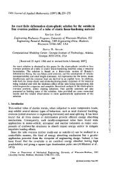
Figure 2 shows plots <strong>of</strong> <strong>the</strong> load magnitude vs. <strong>the</strong> center deflecti<strong>on</strong> <strong>for</strong> <strong>the</strong> case<br />
C,/2,/(A/Z) = 1.5 and C2 = 0 obtained <strong>the</strong> above method. For this soluti<strong>on</strong>, six <strong>element</strong>s<br />
2cQ-<br />
I60 -<br />
I20 -<br />
- Exact soluti<strong>on</strong><br />
Ref 18, A6=30, predictorcorrector<br />
method<br />
Present soluti<strong>on</strong>. AP=30<br />
Ref 14, (Modified Hellinger-<br />
Reissner principle). AD*15<br />
Y I I I I I<br />
0 02 04 06 0.6 IO<br />
FIG. 2.<br />
were used over <strong>the</strong> length <strong>of</strong> <strong>the</strong> beam. Also shown <strong>on</strong> <strong>the</strong> same figure are <strong>the</strong> results obtained<br />
by Pian and T<strong>on</strong>g [18] who use an <strong>incremental</strong> approach and <strong>the</strong> potential energy<br />
principle, and those by Pirotin [14] who uses a modified Hellinger-Reissner principle, as<br />
well as <strong>the</strong> analytical soluti<strong>on</strong> <strong>of</strong> Fung and Kaplan [24]. Both Refs. [18 and 141 are six<br />
<strong>element</strong>s over <strong>the</strong> length <strong>of</strong> <strong>the</strong> beam. Also, it should be pointed out that Pian and T<strong>on</strong>g<br />
[ 181. <strong>for</strong> <strong>the</strong> present problem with proporti<strong>on</strong>al loading characterized by <strong>the</strong> load parameter<br />
p,, treat <strong>the</strong> <strong>incremental</strong> equati<strong>on</strong>s obtained by <strong>the</strong> potential energy principle as<br />
ordinary differential equati<strong>on</strong>s with <strong>the</strong> load parameter PO as <strong>the</strong> independent variable:<br />
and use a predictor-corrector method <strong>for</strong> <strong>the</strong>ir soluti<strong>on</strong>. It is found that <strong>the</strong> results obtained<br />
from <strong>the</strong> present method are comparable to <strong>the</strong>se in [18] as to <strong>the</strong>ir accuracy.<br />
Figure 3 shows <strong>the</strong> variati<strong>on</strong> <strong>of</strong><strong>the</strong> center deflecti<strong>on</strong> with respect to load magnitude <strong>for</strong><br />
<strong>the</strong> case C/l,/(A/I) = 3 and C,/2 J(A/I) = O-01, using ten <strong>element</strong>s over <strong>the</strong> length <strong>of</strong> <strong>the</strong><br />
beam. Again, <strong>the</strong> present results were found to be comparable to those in Ref. [17]. Fur<strong>the</strong>r<br />
results from <strong>the</strong> applicati<strong>on</strong> <strong>of</strong> <strong>the</strong> present method to <strong>the</strong> large-displacement <strong>analysis</strong> <strong>of</strong><br />
an inflated toroidal shell will be presented later [25].
1190 SATYANAD~M ATLURI<br />
91s<br />
2. 4c0<br />
z<br />
la<br />
200<br />
- Exact soluti<strong>on</strong> <strong>for</strong> c,=O<br />
A Ref. 18, A$=300. predictor<br />
corrector method<br />
0 Present soiutl<strong>on</strong>. A6830<br />
FIG. 3<br />
CONCLUSIONS<br />
A c<strong>on</strong>sistent variati<strong>on</strong>al <strong>for</strong>mulati<strong>on</strong> <strong>of</strong> <strong>the</strong> <strong>hybrid</strong> <strong>stress</strong> <strong>finite</strong> <strong>element</strong> <strong>model</strong> <strong>for</strong><br />
<strong>analysis</strong> <strong>of</strong> large deflecti<strong>on</strong> problems, in c<strong>on</strong>juncti<strong>on</strong> with an <strong>incremental</strong> approach, is<br />
presented. The c<strong>on</strong>cept <strong>of</strong> initial <strong>stress</strong>es is imployed. In each <strong>incremental</strong> step, <strong>the</strong> assumed<br />
<strong>incremental</strong> Piola-Kirch<strong>of</strong>f <strong>stress</strong>es satisfy <strong>the</strong> linearized <strong>incremental</strong> equilibrium equati<strong>on</strong>s<br />
in <strong>the</strong> interior <strong>of</strong> each <strong>finite</strong> <strong>element</strong>; whereas, a compatible <strong>incremental</strong> displacement<br />
field is assumed at <strong>the</strong> boundary <strong>of</strong> each <strong>element</strong>. A check <strong>on</strong> <strong>the</strong> equilibrium <strong>of</strong><br />
initial <strong>stress</strong>es in <strong>the</strong> current reference geometry, be<strong>for</strong>e <strong>the</strong> additi<strong>on</strong> <strong>of</strong> a fur<strong>the</strong>r loadincrement,<br />
is included to improve <strong>the</strong> numerical accuracy. The method leads to an <strong>incremental</strong><br />
stiffness matrix and is easily adaptable to existing computer programs,using <strong>the</strong><br />
stiffness approach.<br />
Since <strong>the</strong> <strong>hybrid</strong> <strong>stress</strong> <strong>model</strong> has proven to be a valuable tool in <strong>the</strong> linear <strong>analysis</strong><br />
<strong>of</strong> complex problems such as sandwich plates and shells, and problems with singularities<br />
[Refs. 14 and 111, it can be expected to be <strong>of</strong> equal value in large deflecti<strong>on</strong> problems.<br />
Present results <strong>for</strong> <strong>the</strong> large deflecti<strong>on</strong>s <strong>of</strong> a shallow beam show good agreement with<br />
existing results using displacement <strong>model</strong>s. Fur<strong>the</strong>r results <strong>on</strong> <strong>the</strong> applicati<strong>on</strong> <strong>of</strong> <strong>the</strong><br />
present method to <strong>the</strong> <strong>analysis</strong> <strong>of</strong> a toroidal shell will be presented later.<br />
Acknowledgements-The author wishes to thank Pr<strong>of</strong>essor T. H. H. Pian <strong>of</strong> MIT. and Pr<strong>of</strong>essor K. Washizu<br />
<strong>of</strong> <strong>the</strong> University <strong>of</strong> Tokyo <strong>for</strong> many helpful comments and suggesti<strong>on</strong>s.<br />
REFERENCES<br />
[I] T. H. H. PUN and P. TONG, Basis <strong>of</strong> <strong>finite</strong> <strong>element</strong> method <strong>for</strong> solid c<strong>on</strong>tinua. Inf. J. Numerical Methods<br />
Engng 1 (l), 3-28 (1969).<br />
[2] S. ATLURI and T. H. H. PIAN, Theoretical <strong>for</strong>mulati<strong>on</strong> <strong>of</strong> <strong>finite</strong> <strong>element</strong> methods in <strong>the</strong> linear-elastic <strong>analysis</strong><br />
<strong>of</strong> general shells. J. Struct. Mech. 1 (I), l-43 (1972).<br />
[3] J. T. ODEN, Finite Elements <strong>of</strong>N<strong>on</strong>linear C<strong>on</strong>tinua. McGraw-Hill (1971).<br />
[4] T. H. H. PUN, Derivati<strong>on</strong> <strong>of</strong> <strong>element</strong> stiffness matrices by assumed <strong>stress</strong> distributi<strong>on</strong>s. AIAA J. 2 (7),<br />
1333-1336 (1964).
On <strong>the</strong> <strong>hybrid</strong> <strong>stress</strong> <strong>finite</strong> <strong>element</strong> <strong>model</strong> 1191<br />
[5j T. H. H. PUN and P. TONG, Rati<strong>on</strong>alizati<strong>on</strong> in deriving <strong>element</strong>s stiffness matrix by assumed <strong>stress</strong> approach.<br />
Proc. 2nd C<strong>on</strong>f. <strong>on</strong> Meeting Methods in Structural Mechanics. pp. 461-471. AFFDL-TR-68-150, WPAFB,<br />
Ohio (I 968).<br />
[6-j J. P. WOLF, Programme STRIP pour le calcul des structures en surface porteuse. Bull. Tech. Suesse Romande<br />
Luussanese94 (17). 381-397 (1971).<br />
[TJ R. T. SEVERN and P. R. TAYLOR, The <strong>finite</strong> <strong>element</strong> method <strong>for</strong> flexure <strong>of</strong> slabs when <strong>stress</strong> distributi<strong>on</strong>s<br />
are assumed. Proc. Institute <strong>of</strong> Civil Engineers 36. 153-l 70 (1966).<br />
[8] R. J. ALLW~~D and G. M. M. CORNES. A polyg<strong>on</strong>al <strong>finite</strong> <strong>element</strong> <strong>for</strong> plate bending problems using <strong>the</strong><br />
assumed <strong>stress</strong> approach. Int. J. Numerical Methods Engng 1, 135-149 (1969).<br />
[9] Y. YAMADA, S. MAKAGIRI and K. TAKATSUKA, Analysis <strong>of</strong> St. Venant torsi<strong>on</strong> problem by a <strong>hybrid</strong> <strong>stress</strong><br />
<strong>model</strong>. Paper presented at Japan-US. Seminar <strong>on</strong> Matrix Methodr <strong>of</strong> Structural Analysis and Design,<br />
Tokyo, 25-30 August (1969).<br />
[lo] M. TANAKA, Development and Evaluati<strong>on</strong> <strong>of</strong> a Triangular Thin Shell Element Based up<strong>on</strong> a Hybrid Stress<br />
Model. Ph.D. Thesis, Massachusetts Institute <strong>of</strong> Technology, June (1970).<br />
[I 1] S. T. MAU, T. H. H. PUN and P. TONG. Laminated thick plate and shell <strong>analysis</strong> by <strong>the</strong> assumed <strong>stress</strong><br />
<strong>hybrid</strong> <strong>model</strong>. Paper presented at <strong>the</strong> Army Symposium <strong>on</strong> Solid Mechanics, Ocean City, Maryland, 3-5<br />
October (1972).<br />
[12] T. H. H. PUN, P. TONG and C. H. LUK, Elastic crack <strong>analysis</strong> by a <strong>finite</strong> <strong>element</strong> <strong>hybrid</strong> method. Paper<br />
presented at <strong>the</strong> 3rd C<strong>on</strong>ference <strong>on</strong> Matrix Methods in Structural Mechanics, WPAFB, Ohio, 19-21 October<br />
(1971).<br />
[l3] H. R. LUNDGREN, Buckling <strong>of</strong> Multilayer Plates by Finite Elements. Ph.D. Thesis, Oklahoma State<br />
University (1967).<br />
[l4] S. D. PIROTM. Incremental Large Deflecti<strong>on</strong> Analysis <strong>of</strong> Elastic Structures. Ph.D. Thesis, Massachusetts<br />
Institute <strong>of</strong> Technology, Department <strong>of</strong> Aer<strong>on</strong>autics and Astr<strong>on</strong>autics (1971).<br />
[15] T. H. H. PUN. Hybrid <strong>model</strong>s. Paper presented at Int. Symposium <strong>on</strong> Numerical and Computer Methods in<br />
Srrucrural Mechanics, University <strong>of</strong> Illinois at Urbana. Champaign, 8-10 September (1971).<br />
[16] T. H. H. PIAN. Finite <strong>element</strong> methods by variati<strong>on</strong>al principles with relaxed c<strong>on</strong>tinuity requirements.<br />
ht. C<strong>on</strong>ference <strong>on</strong> Variati<strong>on</strong>al Method in Engineering, Southampt<strong>on</strong>, England, 25-29 September (1972).<br />
[l7] L. D. HOFMEISTER, G. A. GREENBAUM and D. A. EVENSEN, Large strain, elastic-plastic <strong>finite</strong> <strong>element</strong><br />
<strong>analysis</strong>. AIAA J. 9 (7), 1248-1255 (1971).<br />
[18] T. H. H. PIAN and P. T<strong>on</strong>g, Variati<strong>on</strong>al <strong>for</strong>mulati<strong>on</strong> <strong>of</strong> <strong>finite</strong>-displacement <strong>analysis</strong>. M.I.T., ASRL-TR-<br />
144-5, November (1970).<br />
[193 J. A. STRICKLIN, W. E. HAISLER and W. A. v<strong>on</strong> RIESMAN. Texas A & M University, Aerospace Engineering<br />
Department Report 70- 16, August ( 1970).<br />
[20] K. WASHIZU, Incremental <strong>for</strong>mulati<strong>on</strong> <strong>of</strong> a n<strong>on</strong>linear problem in solid mechanics. Recent Aduances ii<br />
Matrix Melho& <strong>of</strong> Structural Analysis and Design, edited by R. H. GALLAGHER et al., pp. 25-27, VAH<br />
Press (1971).<br />
[2l] K. WASHIZU. Variati<strong>on</strong>al Principles in Elasticity and Plasriciry. Pergam<strong>on</strong> Press, Ox<strong>for</strong>d (1968).<br />
[22] C. TRUE~DELL and R. A. TOUPIN, The classical field <strong>the</strong>ories. Han&uch der Physik. Vol. III, Part I. Springer<br />
(1960).<br />
[23] A. E. GREEN and J. E. ADKINS, Large Elastic De<strong>for</strong>mati<strong>on</strong>s. The Clarend<strong>on</strong> Press, Ox<strong>for</strong>d (1960).<br />
[24] Y. C. FUNG and A. KAPLAN, Buckling <strong>of</strong> Low Arches and Curved Beams <strong>of</strong> Small Curvature. NACA<br />
TN 2840. 1952.<br />
[251 A. L. DWK and S. ATLUIU, Static <strong>analysis</strong> <strong>of</strong> an aircraft tire. To be published.<br />
(Received 27 July 1972; revised 8 February 1973)<br />
A&JMWT--fiaeTC9 o606ueHHe hwnenw K<strong>on</strong>eworo 3neMeiiTa co crdeuantiblMH HanpnXeHnnMn nnn 3anaqu<br />
c 60nbumw4 nporu6aMa. 3ra M<strong>on</strong>enb nepa<strong>on</strong>aqanbno npeanowceiia lli4atioM pnn nHHeknbix 3aaa9. a<br />
paMKaX ManblX nepeMe”,eHMk. kkllOnb3y,OTCR pa3HOCTHMR nOAXOn M IlOHRTHIl Ha’WlbHblX HanpRXfeHWfi.<br />
llpti130~~Tcn npouecc npoaepau pawtoaecm Ann w2xomoro C~CTORHH~. panawe AO6aBneHWI no6aeornorO<br />
npnpaueHHn Harpy3Kw. AaIoTcn npmep w 06cymeHHe pe3ynbTaToa.